IMT to Satellite Stochastic Interference
Modeling and Coexistence Analysis of
Upper 6 GHz Band Service
Abstract
The surging capacity demands of 5G networks and the limited coverage distance of high frequencies like millimeter-wave (mmW) and sub-terahertz (THz) bands have led to consider the upper 6GHz (U6G) spectrum for radio access. However, due to the presence of the existing satellite (SAT) services in these bands, it is crucial to evaluate the impact of the interference of terrestrial U6G stations to SAT systems. A comprehensive study on the aggregated U6G-to-SAT interference is still missing in the literature. In this paper, we propose a stochastic model of interference (SMI) to evaluate the U6G-to-SAT interference, including the statistical characterization of array gain and clutter-loss and considering different interference modes. Furthermore, we propose an approximate geometrical-based stochastic model of interference (GSMI) as an alternative method to SMI when the clutter-loss distribution is unavailable. Our results indicate that given the typical international mobile telecommunication (IMT) parameters, the aggregated interference power is well below the relevant protection criterion, and we prove numerically that the GSMI method overestimates the aggregated interference power with only 2dB compared to the SMI method.
Index Terms:
satellite communication, U6G, 6G, aggregated interference, stochastic geometryI Introduction
The coexistence of satellite (SAT)communications with fifth-generation (5G)and beyond 5G (B5G)base station (BS)operating in the upper 6GHz (U6G)frequency is an arising issue due to the growing interest in new bands to increase capacity in densely populated areas [1, 2, 3, 4]. Studies demonstrate that the usage of the upper mid-band is necessary to fulfill the requirements of the downlink of 5G [5]. At the same time, around of the benefit foreseen for 5Gmid-bands will not be exploited in the absence of a new mid-bands spectrum assignment [6]. These additional frequencies provide large bandwidth, in excess of 100 MHz, while characterized by a smaller path loss compared to millimeter-wave (mmW)5G[7]. The deployment of new U6Gsystems might affect the operation of SATs already in place that use these frequency bands in uplink [7], such as C-band (4-8 GHz) and X-band (8-12 GHz) [8]. Even if the emission of a single BSserving all user equipment (UE)has a negligible impact on SAT, the aggregation of the interference from a large number of BSs in a large area (e.g., the satellite footprint (SATFP)on Earth) might be harmful. In [9], the effect of the interference on geosynchronous synthetic aperture radars has been studied in the context of remote sensing in the C-band. However, the sources of interference are different w.r.t the international mobile telecommunications (IMT).
Currently, there are no comprehensive studies regarding the statistical analysis of aggregated interference from BSs, observed by the SATs in the U6Gbands. The coexistence analysis between IMT-2020 and SATsystems has been widely studied (see, e.g., [10, 11, 12, 13, 14]) mostly for mmWbands (24.25 and 86 GHz), and in the context of relevant agendas (see e.g., [15] or international telecommunications union (ITU)agenda WRC-23 item 1.2). The previous works usually target the aggregated interference in the SATFPconsidering only the direct BS-SATpath. Moreover, they all consider the same propagation model, valid for frequencies above 10 GHz (see [16] for further details). Therefore, it is clear that existing interference modeling approaches cannot be readily extended to the U6Gspectrum, since (i) the propagation model is not appropriate for frequencies GHz, and (ii) different interference modes are typically neglected. The term interference mode is herein used for any propagation that ends up toward the SAT, including the direct BS-SATpath or reflections (from the ground or buildings towards the SAT).
The problem of interference estimation in communication systems involves the modeling of both the U6Gdevices (deployment, functioning, antennas, etc.) and propagation for the involved frequencies and environments. Several guidelines to evaluate the compatibility between terrestrial and space stations are provided in the literature. The work in [17] presents a methodology for modeling IMT-Advanced, namely fourth-generation (4G), and IMT-2020 (5G), networks, and systems for general coexistence studies. It details the simulation setup, including the modeling of network topology and antenna arrays. The methodology is based on the characteristics of IMT-advanced systems [18].
Besides system modeling, it is necessary to determine a suitable propagation model for earth-space interference evaluation [19], including all the relevant phenomena such as clutter loss, which is an additional loss with respect to the path-loss, created by the diffraction, reflection, or scattering of the buildings and vegetation in the vicinity of the BSs. An empirical model for the cumulative distribution function (CDF)of the clutter loss is reported in [16], for earth-space links working above 10 GHz. This latter model can be used when the geometry of the scenario is not known. In contrast, when prior information on the environment is available, e.g., statistical characterization of the geometrical features, the stochastic model in [20] might be applied, provided that appropriate modifications are made to extend its validity below 10 GHz.
The main contribution of this paper is the development of a stochastic method that can be used to evaluate the aggregate interference at the SATfrom U6G terrestrial BSs. The proposed method is general since it does not constrain the analysis to any specific scenario. The detailed contributions are listed in the following:
- •
We develop an stochastic model of the interference (SMI)towards a SATfrom a set of micro and macro BSs, based on a stochastic description of the BSarray gain and clutter loss, calculated according to the geometrical distribution of a given region. We use a characteristic function (CF)-based approach, to efficiently aggregate all the interference power, from different types of BSs, when serving both indoor and outdoor UEs, to ultimately yield a methodology for estimating the aggregated interference power from the SATFP.
- •
We propose a geometry-based stochastic model of the interference (GSMI)method to estimate the aggregated interference at the SATwhen no clutter-loss statistics are available. The GMSI method leverages the environment’s geometrical statistics.
- •
We provide numerical examples of the interference CDFfor U6Gservice with the SMI and GSMI methods. Our results demonstrate that, given typical parameter values, the aggregated interference power from U6Gis well below the interference to noise ratio (INR)protection criterion, while it is relevant only for extreme values of the employed parameters. We show that the GSMI results overestimate the interference power density by only dB with respect to SMI results, on aggregate for the SATFP.
Organization: The remainder of the paper is organized as follows: in Sec. II we present the system model. In Sec. III and Sec. IV, the methodology for modeling the interference from a single BSand from BSs in a large region are presented, respectively. The distribution of the array gain and clutter-loss are discussed in Sec. V and Sec. VI. In Sec. VII, the process of extracting the geometrical statistics is discussed. The numerical results are in Sec. VIII and the paper is concluded in Sec. IX.
II System Model

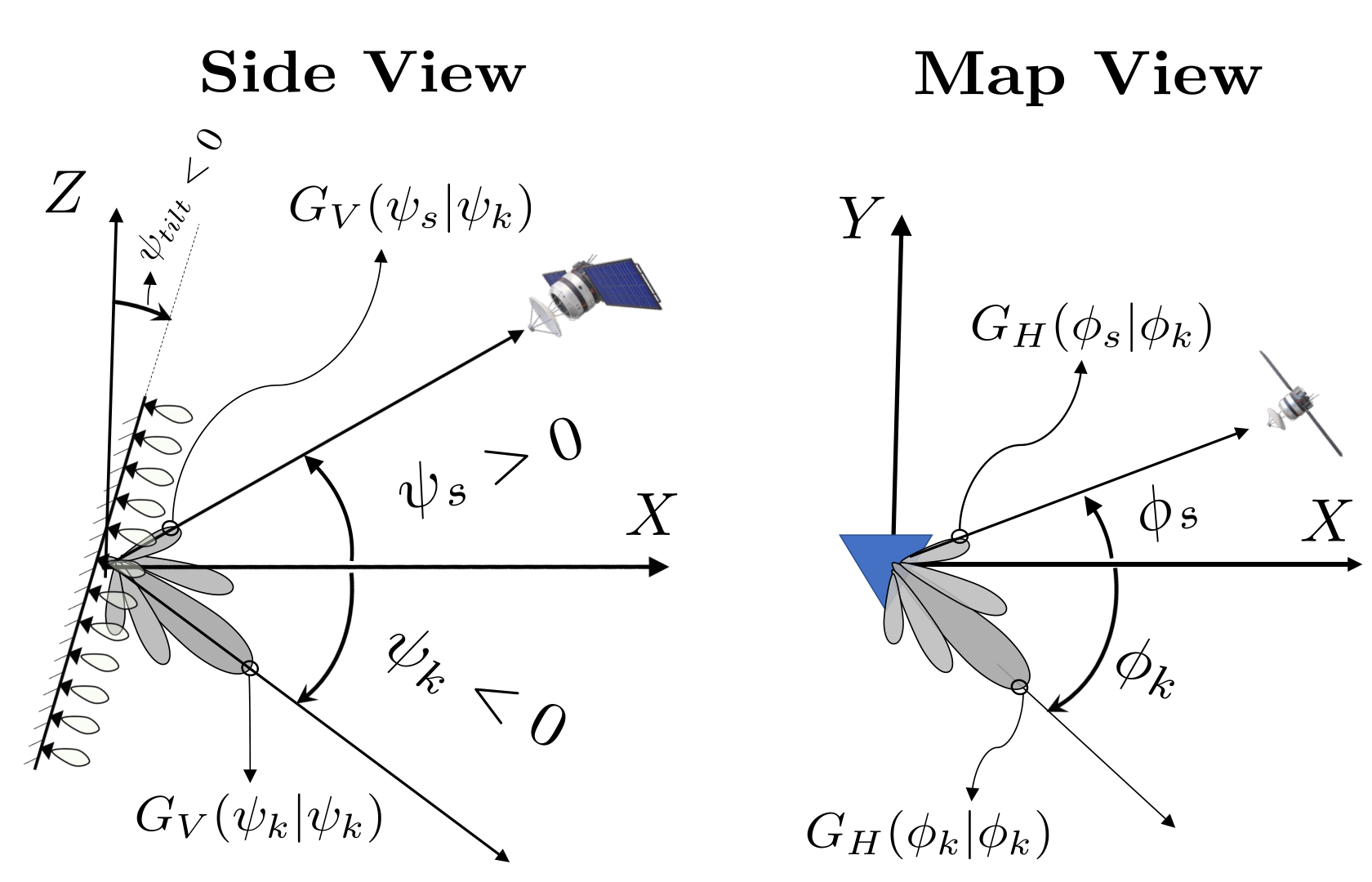
Modeling the aggregated interference to a SATfrom a set of BSs requires both geometrical and propagation considerations. Let us consider the scenario in Figure 1, where a single BSat height is causing interference to the SATwhile serving a single-antenna ground UE. The coordinate system is such that an arbitrary set of angles , consists of azimuth angle deg, defined as clockwise positive from North, and elevation angle defined as deg relative to the ground plane, located at the BSheight. The SAT, given a longitude and latitude of observation, is identified by the angle of departure (AoD). In this setting, correspond to any interference mode that first bounces on the ground. The same coordinate system is used for the served UE at . A set of stochastic parameters characterizes the environment, UE, and the BSdistributions, including: (i) inter-building distance ; (ii) BS-building distance; (iii) the BSheight ; (iv) buildings height ; (v) UEs height . The signal received by the -th UE from a single BSis
| (1) |
where is the Tx signal, is the array gain toward the UE of interest, when the BSarray is designed to points toward (Fig .2), is the Tx power and the path-loss for distance , including any shadowing and fading and is the noise amplitude. For a given position and height of the BS, the signal (1) toward the UE, generates interference at SAT. This is originated from either the direct path (i.e. at angle ), and/or from other interference modes. For example, the signal might be reflected by ground/buildings toward the SAT, or it might be diffracted by vegetation/building edges. Let denote the AoDof the rays in -th propagation mode, which is a function of (e.g., for direct BS-SAT propagation mode, it is ). The interfering signal received by the SAT, when the -th BSis serving the -th UE (-th interference mode) is
| (2) |
where is the BS array gain toward when it is designed to points to , is the clutter loss between the BSand SAT, is the additive white Gaussian noise with power spectral density (PSD) over bandwidth , while consists of all the phenomena above the terrain as
| (3) |
where , , and are respectively the SATantenna gain, the free space path loss, and the loss due to polarization mismatch. The dependence of the array gain and clutter loss on the set of geometrical parameters , and the interference modes is detailed in Sec. V and Sec. VI. Note that the beam spread loss, which is the loss caused by refractive effects of the atmosphere, is neglected since it is only relevant for very small elevation angles [21], and atmospheric gases absorption is typically neglected around 6 GHz [8, 22].
Although the largest part of the aggregated interference comes from the direct BS-SATpath, all the other interference modes cannot be neglected, otherwise, the interference is underestimated.
The aggregated interference power caused by total BSs each serving possible UEs, through possible interference modes, is
| (4) |
where is the single interference power contribution. In practice, the number of served UEs is not deterministic, and the aggregation over all the served UEs can be replaced by modeling the transmit power with an appropriate probability density function (PDF)and the BSloading factor. Thus, herein the UE index in (4) will be dropped with the corresponding summation.
BSs can be modeled as transmitting with full power (On) or not transmitting at all (Off) [17], with a loading factor defined as the percentage of the BSs that are randomly chosen as active. Furthermore, each BStransmit only a fraction of total time , due to employing time division duplex (TDD). Each BSis either a macro BSor a micro BS, as shown in Fig. 3. Macro BSs employ larger array sizes, organized in three sectors to cover multiple cells, a higher transmitter power , and a larger height compared to micro BS. We assume, without any loss of generality, that macro BSs are placed on top of the tallest building in each area [17], for coverage purposes. Differently, micro BSs have a single sector, and they are characterized by a reduced Tx power and are mostly aimed at boosting coverage and capacity at cell edges. Thus, for mere modeling purposes, we assume the micro BSis located on the ground, at the furthest distance from the macro one. Considering a single BS, its height from ground as well as its position with respect to surrounding buildings can be regarded as random. This affects the modeling of the interference modes toward the SAT, which can be evaluated in a probabilistic framework, using the geometrical statistics of the environment.
III Statistical Model of Interference from a Single BS
We propose a statistical framework to evaluate the interference at the SAT, using both SMIand GSMI. In the SMImethod, all the possible interference modes (from every possible bounce of the rays) are considered to occur, and each propagation path is subject to a specific clutter loss, with a corresponding probability distribution. In the GSMImethod instead, the interference modes are limited to the significant ones, each of these occurring with a specific probability, while the clutter loss is not considered. A main difference between the two methods is that the PDFof the clutter loss in the SMI method is achieved by ray tracing. Instead, the GSMI makes use of stochastic geometry to approximate clutter loss.

III-A Stochastic model of interference (SMI)
In the SMI method, the interference is evaluated by considering every possible interference mode that reaches the SAT with any number of bounces. The SMI method requires knowledge of the PDFof both array gain and clutter-loss for every propagation mode. For the -th propagation mode, the rays departing from the BSwith specific AoD reach the SATexperiencing a different array gain and clutter loss. Given the geometrical stochastic parameters , the interference power at the SAT from the -th BScan be evaluated by adopting (2) in dB scale as
| (5) |
where denotes the value of in dB scale, is the clutter gain, inverse of the clutter loss defined in (2). The corresponding PDFof is obtained as (6) (bottom of the page) by means of the logarithmic convolution [23].
| (6) |
The PDFof the interference power in linear scale, i.e. , can be easily converted from dB scale as indicated in [23]. Given the joint PDFof the geometrical parameters , , we can write:
| (7) |
where is the expectation of x over . Note that is conditioned to a given satellite azimuth , as detailed in Sec. VII. The analysis of the interference power is carried out using the CFof the , defined hereafter as . The usage of the CFis preferred in interference analysis [24, 25], because it always exists when it is a function of a real-valued argument [26], and cumbersome convolution operations can be converted to simpler products. The aggregated interference from -th BSto SAT, , is the independent summation (in linear scale [27, 28]) over the possible interference modes, whose CFis achieved as
| (8) |
This CFis used in Sec. IV for aggregation of interference coming from all BSs in a given region.
III-B Geometry-based stochastic model of interference (GSMI)
The GSMI method is an alternative to SMI whenever the PDFof clutter gain in (6) is not available. Typically, is obtained by means of exhaustive and computationally intensive ray-tracing simulations, which could be unavailable in some cases, especially over large areas such as the SATFP. With GSMI, we assume that the interference at the SAT comes from a limited set of interference modes. These are the following: (i) direct path (DP); (ii) single-building (SB) reflection; (iii) double building (DB) reflection; (iv) ground reflection (GR); (v) ground and building (GB) reflection, while other reflections are neglected due to higher propagation losses. Herein, we denote the set of considered modes as . The -th interference mode can occur with a certain probability , that depends on the system parameters as well as on the BStype. For instance, micro BScan experience all the interference modes, while for macro BS, located on the rooftop, SB and DB, typically do not occur. Note that, one or more interference modes might occur simultaneously, and thus we have
| (9) |
Appendix A reports the derivation of and further information.
Unlike the SMI method, where the possible interference modes is usually large, here the interference is limited to only 5 contributions (3 in case of rooftop BS). The average probability of occurrence of the -th mode can be computed as
| (10) |
The interference power and its PDFin each interference mode from -th BS, , is achieved with (5), (6) and (7) by removing the clutter gain and its PDF. However, it must be noted that, since every interference mode considered in the GSMI method has a specific occurrence probability, the PDF of the interference is conditioned to the occurrence of the corresponding -th mode. Thus, this difference can be modeled by slightly modifying (8), yielding
| (11) |
This modification is justified in Sec. IV when aggregating the interference coming from all BSs in a given region.
IV Aggregation of Multiple BS
The interference power generated by a single BSis then aggregated over multiple BSsuch as over a city, or a large geographical region (e.g., the whole SATFP).
IV-A Aggregation over a city
The first aggregation step is to consider a whole area of a city . The CF of the aggregated interference power at SAT from all the BSs (either macro or micro) is computed as
| (12) |
where is the effective average number of BSs in the city, is the density of the macro/micro BSs, and is the BSpower loading factor based on the ITUrecommendation [18] as the percentage of all the BSs considered to be working at full power with maximum Tx power, and is the BSTDDactivity factor. Model (12) endorses that in the GSMI method, every interference mode occurs on average times, which is the rationale behind in (11).
The general aggregation rule (12) can be specialized to derive the CFin more specific cases, i.e., differentiating between different BS types (macro and micro) and UE locations (indoor vs. outdoor). The BStype affects the interference mostly through the height , which changes from macro to micro and affects the PDFof the array gain. Similar behavior is expected for the UE location (described by average UE height ), as UEs located outdoor have while indoor UEs may have a much higher height from the ground. These assumptions affect the array gain and clutter loss. For example, let us consider the case of micro BSs, and assume that all the UEs are indoor. In this case, we have a constant BS height m by assumption (see Sec. II), and the UEis bound to the building height as . The former term influences directly the clutter loss (see Sec. VI), while the second indirectly affects the array gain, defining a specific AoD toward the k-th UE, . We denote the aggregated interference under these assumptions as and its CFwith . The table Isummarizes the four different interference contributions over an entire city. Let be the fraction of outdoor UEs and be the fraction of indoor UEs. The overall CFof the aggregated interference power is
| (13) |
Note that all of the micro and macro BSs coexist simultaneously, while a fraction of UEs is indoor/outdoor. The corresponding PDF is computed as the inverse Fourier transform of the CF as
| (14) |
In practice is evaluated using the Gil Pelaez theorem of inversion [29], which can be carried out numerically [30].
| BSType | UE Type | Notation |
| Micro BS | Indoor | and |
| Micro BS | Outdoor | and |
| Macro BS | Indoor | and |
| Macro BS | Outdoor | and |


IV-B Aggregation over the SATFP
In case the aggregation area is larger than a single city, different locations on Earth’s surface see the SATunder different elevation angles. This causes the interference contribution from the same BSmodel to be different based on latitude and longitude location [10]. To obtain the total aggregated interference, we first identify the regions that share similar link budget parameters towards the SAT, i.e., the same elevation angle and the same SATantenna gain. These regions are called Geographic Clusters (GC).
Let us consider the example of a SAToccupying an orbital location (0N, 5E) in a geostationary orbit and having the uplink antenna pointing at Nadir. Also, assume that the locations on Earth’s surface are discretized by defining a tessellation of pixels of deg along latitude and longitude. Fig .5a shows the pixels inside the 3 dB SATFPassuming the antenna pattern model as defined in [31], with SATgain quantized in steps of 1 dB. The maximum gain and 3 dB beamwidth (22 dBi and 15∘ respectively) are taken from ITU WP4 discussions and, assuming a parabolic antenna mounted on the satellite [32]. Assume that the set of GCs are , where denotes the -th CG. The number of GC is . Now, the GCs inside SATFPwill observe the SATunder different angles identified by azimuth and elevation pairs , as depicted in Fig .5b. Since the effect of the azimuth, is averaged out due to the fact that the BSs are assumed to be randomly oriented throughout a large region (see Sec. V), only the impact of the SATelevation is of interest. In Fig .5b, the elevation angle of the SATseen from Earth is depicted for each pixel with an angle quantization of deg. Each GC can thus be represented as a unique pair . The GCs obtained with the selected resolution are reported in Fig .5c. To compute the aggregated interference coming from the SATFP, for each GC we find the CF of its interference contribution following the procedure detailed in Sec. III. Then we aggregate the CFs of all the GCs to find the overall result as
| (15) |
where is the CF of interference from the -th GC, computed with (13), using the corresponding SATRx gain on each GC and the average number of BSs in the -th GC . The latter is the product of the GC area , the average density of the macro BSs , the BSloading factor , TDDactivity factor , while and are parameters defined by ITU [33], to establish a bond between amounts of BS and large-scale land areas in the order of SATFP, where is the percentage of built area, and is the percentage of the area from a certain type, e.g., urban, suburban, and etc. Here we consider urban area type.
IV-C Interference protection criterion
Given the interference power and signal bandwidth , the interference protection criterion, is based on the INRdefined as [35]:
| (16) |
where is the noise PSDwith as the Boltzmann constant and is the SAT Rx system temperature [36]. The SAT is protected from interference whenever interference threshold criterion , with being a threshold specified by satellite regulators. In [37], the is given for mmWin the range of K depending on different parameters, while the calculations in [9], demonstrate system thermal noise of around K in the C-band.
V Stochastic Array Gain
This section details the modeling of the array gain and its PDF. We consider generic rectangular panels for each BS sector, each configured with vertical and horizontal antennas. The equivalent isotropically radiated power (EIRP)is therefore defined as
| (17) |
where is the sub-array size (number of antennas connected to a single RF chain) in a hybrid digital-analog antenna array, and the Tx power , is related to a single RF chain (i.e., a single power amplifier (PA)) [17, 18], while corresponds to a fully digital antenna array. A feeder loss can be added to further reduce the effective EIRP as indicated in [38]. The horizontal and vertical gains assigned toward a generic azimuth and elevation steering toward the -th UE are
| (18) | ||||
| (19) |
where: (i) and are the horizontal and vertical element directivity gains [39], respectively, (ii) and are the horizontal and vertical ULA response vectors, respectively, (iii) and are the conventional horizontal and vertical beamforming, indicates the hermitian of vector b, and is the orientation of the serving BSpanel that is perceived by the SATas . Note that corresponds to any BSpanel that observes the target azimuth within the electromagnetic (EM)shielding limit while serving the -th UE, as , where deg. With such an assumption, it is apparent that only one of the panels of the macro BSis capable of interfering with while serving a UE at . In the case of micro BS, depending on the number of the BSs and their orientations, one or multiple BSs might be interfering. The total gain is
| (20) |
The corresponding array gain for -th interference mode with AoD is denoted as , that for the direct BS-SAT link would be . The PDFof the array gain is achieved by Monte-Carlo simulations, given the random . This PDFis for the array gain toward a single UE, while the number of the served UEs affects the Tx power and the BSloading factor, rather than the array gain. Note that the random AoD of the k-th UE , is inherently a function of environment parameters , as it depends on the cell size, random 2D position of the UEs within the cell, the distribution of the UEs height, and the distribution of the BSheight.
VI Stochastic Clutter Loss
Clutter is the term herein used to indicate objects that are on the Earth’s surface, but are not the terrain itself, i.e. buildings and vegetation. Clutter loss consists of reflection loss and diffraction loss , properly combined as indicated in [20]. Quantifying clutter loss is not trivial, since it is strongly dependent on both environment and geometry of the link of interest. The target AoDalso plays a crucial role [40, 41]. One possible approach is to use a ray tracer to evaluate clutter loss via deterministic simulation, but the computational load makes this method applicable to limited areas only, yielding site-specific results that are not general enough [40]. As previously mentioned, ITU recommendation [20] contains guidelines to perform stochastic Monte Carlo simulation of clutter loss statistics, making use of environment geometrical data and stochastic geometry to evaluate the CDFof clutter loss at a given elevation angle . Some of the stochastic parameters of the environment that serve as the input for this method are BS height, the material of the buildings/ground, and some specific percentiles of the inter-building distances and buildings’ height.
Although the statistical nature of the approach in [20] is very much suited to our model, there are some limitations that can affect the applicability of this model: the model is not considered valid below 10 GHz, a limited number of reflections and diffraction are considered (up to two), the reflection coefficients are not dependent on angles of incidence and polarization. Furthermore, the main drawback is that this method is designed for only the direct BS-SAT link, and it does not provide distinct clutter loss statistics for different interference modes. This is while the SMI method require a distinct clutter loss corresponding to the -th propagation mode. In this regard, one could resort to the model proposed in [34] as an extension of [20], where the aforementioned limitations are overcome, considering positive and negative interference modes. Positive modes are all the modes that leave the BSupward with elevation and negative modes are all the modes that leave the BSdownward with elevation , i.e. ground reflection modes. Fig. 6 shows the clutter-loss, diffraction-loss and reflection-loss, given the extracted geometrical statistics of Milan, when the BSis located at m height.
Remark: Being more specific regarding diffraction and reflection, it can be understood that the GSMImethod, in fact, mimics the effect of diffraction loss, in a hard decision manner, i.e., a ray is in line-of-sight (LOS)mode or fully blocked in a stochastic manner. However, in some cases, reflection loss is dominant as seen in Fig 6. Thus, in order to take the reflection loss into account (if it is available), one can repeat the same procedures of GSMI method, by replacing and with reflection gain and its PDF in relations (5) and (6), respectively.


VII Geometrical Statistics
As shown in Section II, the set of geometrical parameters is required to calculate the interference power. These parameters affect both the array gain and clutter loss (see Sec. V and Sec. VI). Furthermore, they are necessary to compute the occurrence probability in the GSMI method as (10). These geometrical statistics used are extracted using a pseudo-3D or 2.5D approach [42, 43], where the 3D geometry is split into 2D cross-sections along the SAT azimuth . The city of Milan is taken as a reference, and we generate (i) the PDFs of the buildings’ heights, (ii) the PDFs of the reflection area of each building’s facade, and (iii) the PDFs of buildings’ inter-distance (i.e, streets’ widths), each on a regular azimuth grid with quantization step of deg, using relevant public datasets with further processing [44]. Figure 7a shows an exemplary portion of Milan from the original dataset, where each polygon defines a specific detail of a building with a particular height. Such details are not required, as we are interested in representing only the external buildings’ facades, and some merging processes can be applied to reduce the complexity of the environment while maintaining useful geometrical information. The convexification process is shown in Figure 7a to 7c, where the final convex polygons are associated with average heights and widths, retrieved for each merged building. Although not reported here, it can be shown that the merging-plus-convex approximation of the buildings’ geometry preserves the facades’ area.
From the simplified dataset, we generate the PDFs for each SAT azimuth angle . The buildings’ heights are discretized at m and the PDF is derived from the histogram. Each entry of the histogram is a weighted sum of all the building’s facades of height perpendicular to the azimuth satellite direction , (i.e., that can effectively contribute to the clutter loss) The PDF of the buildings’ reflecting area is evaluated similarly, by using the histogram of occurrence of a certain reflection area , discretized with a step of m2. Differently, the PDF of the buildings’ inter-distance is weighted by the effective visibility region between adjacent buildings, as illustrated in Fig .9. The PDF is again approximated as
| (21) |
where is the inter-distance histogram quantized with step m, but the -th histogram element is now computed as
| (22) |
where is the width of the visibility region of two adjacent buildings with parallel facades and is the average height of the two involved facades. The set , therefore, spans all the pairs of parallel facades at distance and perpendicular to . Fig. 8 shows the distribution of building’s height , inter-building distance , and buildings’ reflection area , given some exemplary SATazimuth deg.
VIII Numerical Results
This section shows the numerical aggregated interference power density for the city of Milan and the SATFP.
VIII-A Simulation setup
The BSarrangement is the same depicted in in Fig .3 (Section II). For each macro cell, we consider 3 single-sector micro BS, for a total of 9 micro BS for each macro BS. Micro BSs are placed at m [18, 14], while macro BSs at m, where is the height of the tallest building in the 3 macro cells pertaining to the same macro BS. The macro cell radius considered is m [18] and the macro BS density is therefore , where is the macro cell’s area. The micro cell radius is assumed to be . Each micro BSserves UEs within , while the rest are served by the macro BS.
The UEs are considered to be randomly located either on the ground (outdoor UEs) and inside the buildings (indoor UEs), according to a 2D random distribution with spatial density [UE/m2] (on the ground plane). Outdoor UEs are assumed to have a constant height meter. Indoor UEs’ height is assumed to be meters, where follows the distribution of the buildings’ height.
| Config. 1 | Config. 2 | |||
| macro | micro | macro | micro | |
| 8 | 4 | 8 | 8 | |
| 8 | 8 | 16 | 8 | |
| 1 | 1 | 2 | 2 | |
| (dB) | 3 | 3 | 3 | 3 |
| (dBm) | 25 | 19 | 22 | 16 |
| EIRP (dBm) | 58 | 46 | 58 | 46 |
| (deg) [39] | 65 | 65 | 65 | 65 |
| (deg) [39] | 65 | 65 | 65 | 65 |
| (deg) | -10 | -10 | -10 | -10 |
| (dBi) [39] | 8 | 8 | 8 | 8 |
Table II shows the array configurations used for macro and micro BSs in this paper. The antenna element directivity model is based on [17, 39], with maximum element directivity gain , vertical and horizontal fields of view of and , respectively, and feeder loss (see Table II). Fig .10, shows an example of the CDFof the array gain for the macro BS toward , averaged over the distribution of the height of the buildings and the height of the UEs, when serving an indoor UE with array configuration 1 of table II. It can be noticed that interference modes characterized by (i.e., reflections from the ground) are characterized by a higher array gain, and, consequently, a larger interference contribution as the BS is tilted towards the ground. Table. III summarizes other relevant simulation parameters.
| Parameter Name | Parameter | Value |
| SAT azimuth | (deg) | 45 |
| central frequency | (GHz) | 6 |
| SAT distance | (Km) | 35000 |
| path loss | (dB) | 199 |
| bandwidth | B (MHz) | 100 |
| Macro cell radius | (m) | 300 |
| SAT Rx temperature [9] | (Kelvin) | 800 |
| threshold INR at [33] | (dB) | -10.5 |
| polarization loss | (dB) | 3 |
| BSloading factor [33] | 20% | |
| TDDactivity factor [33] | 75% | |
| Ratio of urban area type [33] | 5%, 10% | |
| Ratio of built-up areas [33] | 1% |
VIII-B Aggregated interference from the city of Milan
Fig. 11 shows the CDFof the aggregated interference power density, using the SMI method with array configuration 1 (Table II). Given the area of the city of Milan , the equivalent number of BSs with maximum power is . It can be observed that the INR based on the aggregated interference coming from a city of Milan size is much lower than dB.
VIII-C Aggregated interference of SATFP
In order to encompass the interference from the SATFP, we follow the methodology introduced in Sec. IV-B. The corresponding specifications of each GC are shown in Table IV. The values of and are chosen according to [45] and [33], respectively. The average loading factor corresponds to typical values of coexistence studies when the area under study is a large region consisting of hundreds of BSs or more [33].
Fig. 12a and 12b show the median value of the INRusing the array configuration 1, for 8 GCs and the whole SATFP(see Section IV-B), with SMI and GSMI methods. It can be seen that with , the INR is well below the threshold , while only for extremely dense deployments with , would yield an INR level close to . Notice that the SMI method is the baseline model and GSMI is an approximate method that overestimates the interference w.r.t. the SMI by approx. 2 dB.
| 1 | 20 | 3 812 552 | 30 |
| 2 | 20 | 6 654 033 | 40 |
| 3 | 21 | 30 088 | 40 |
| 4 | 21 | 9 203 759 | 50 |
| 5 | 21 | 5 104 969 | 60 |
| 6 | 22 | 4 632 108 | 60 |
| 7 | 22 | 6 869 836 | 70 |
| 8 | 22 | 2 605 246 | 80 |
One way to reduce the aggregated interference power is to increase the number of array antennas on the vertical plane while keeping constant EIRPand preserving the quality of service of the U6Gservice. The consequent reduction of sidelobe’s level diminishes the interference at SAT. Fig. 13 shows the INR for the two array configurations in Table II. The percentile of the INR is decreased by more than 4 dB when using the antenna array configuration 2, i.e., double the antennas on the vertical plane of the macro BS. In this latter case, even the extremely dense deployments with would be well below the . Other solutions to reduce U6Ginterference reduction can be investigated, but it is beyond the scope of this paper [46].
We remark that the numerical results are herein obtained using the statistics of the city of Milan since the statistics of each GC are not available. A more accurate estimation of the level of interference requires accurate knowledge of the distribution of geometric parameters for every different region.
IX Conclusion
In this paper we develop a stochastic model of interference (SMI) to evaluate the aggregated interference power at the SAT in U6G band from a set of BSs belonging to an arbitrarily large geographical area. The SMI is based on stochastic array gain and clutter loss, and it considers different interference modes such as direct path and reflections from buildings and ground. In addition, we propose a geometry-based stochastic model of interference (GSMI) method to be used in the absence of the distribution of diffraction loss and/or reflection loss. We demonstrate, for typical parameters’ values in the context of communications coexistence, that the interference power generated by U6G BSs in typical cases is below the interference thresholds set as tolerable for SATby standardization organizations. Remarkable degrees of freedom for SAT interference reduction is based on how the antenna array and system are designed.
Acknowledgement
The research has been carried out in the framework of the Joint Lab between Huawei and Politecnico di Milano. The authors would like to acknowledge the enlightening discussions and clarifications with Carlo Riva on clutter loss models.
Appendix A Calculation of occurrence probabilities
The occurrence probability of the direct path between BS and SAT can be computed from basic geometrical considerations. Based on Fig. 14, the direct path exists whenever it is not blocked by building 2, thus when . Given the CDFof the buildings’ height, defined as
where is detailed in Sec. VII. The occurrence probability of this interference mode is
Other interference modes are similarly treated, with straightforward modifications, using the image method (see e.g., [47, 48]). The corresponding occurrence probabilities are not reported for brevity.

References
- [1] G. Naik, J.-M. Park, J. Ashdown, and W. Lehr, “Next Generation Wi-Fi and 5G NR-U in the 6 GHz Bands: Opportunities and Challenges,” IEEE Access, vol. 8, pp. 153 027–153 056, 2020.
- [2] Coleago Consulting, “The 6 GHz opportunity for IMT. 5G area traffic demand vs. area traffic capacity supply,” Aug. 2020. [Online]. Available: http://www.coleago.com/app/uploads/2020/09/The-6GHz-Opportunity-for-IMT-Coleago-1-Aug-2020-002.pdf
- [3] US Federal Communications Commission, “Unlicensed Use of the 6 GHz Band, Report and Order and Further Notice of Proposed RulemakingET Docket No. 18-295; GN Docket No. 17-183,” Dec. 2019. [Online]. Available: https://www.federalregister.gov/documents/2020/05/28/2020-11320/unlicensed-use-of-the-6-ghz-band
- [4] Analysis Mason, “Discussion on the 6GHz opportunity for IMT,” Dec. 2019. [Online]. Available: https://www.analysysmason.com/contentassets/2a36d000895f4700a2273d3bfee449bf/discussion-on-the-6-ghz-opportunity-for-imt.pdf
- [5] GSMA, “Estimating the mid-band spectrum needs in the 2025-2030 time frame.” [Online]. Available: https://www.gsma.com/spectrum/wp-content/uploads/2021/07/Estimating-Mid-Band-Spectrum-Needs.pdf
- [6] GSMA, “Vision 2030: Insights for Mid-band Spectrum Needs.” [Online]. Available: https://www.gsma.com/spectrum/wp-content/uploads/2022/07/5G-Mid-Band-Spectrum-Needs.pdf
- [7] L. Nan, G. Chunxia, and W. Dapeng, “Considerations on 6 GHz Spectrum for 5G-Advanced and 6G,” IEEE Communications Standards Magazine, vol. 5, no. 3, pp. 5–7, 2021.
- [8] L. Ippolito, “Radio propagation for space communications systems,” Proceedings of the IEEE, vol. 69, no. 6, pp. 697–727, 1981.
- [9] Y. Li, A. Monti Guarnieri, C. Hu, and F. Rocca, “Performance and Requirements of GEO SAR Systems in the Presence of Radio Frequency Interferences,” 2018.
- [10] Y. Cho, H.-K. Kim, M. Nekovee, and H.-S. Jo, “Coexistence of 5G With Satellite Services in the Millimeter-Wave Band,” IEEE Access, vol. 8, pp. 163 618–163 636, 2020.
- [11] Y. Cho, H. Kim, D. K. Tettey, K.-J. Lee, and H.-S. Jo, “Modeling Method for Interference Analysis between IMT-2020 and Satellite in the mmWave Band,” in 2019 IEEE Globecom Workshops (GC Wkshps), 2019, pp. 1–6.
- [12] S. Liu, X. Hu, and W. Wang, Frequency Sharing of IMT-2020 and Mobile Satellite Service in 45.5–47 GHz, 01 2018, pp. 127–135.
- [13] V. J. Richard Rudd, Selcuk Kirtay, “Coexistence of terrestrial and satellite services at 26 GHz,” plumconsulting.co.uk, 2019.
- [14] Z. Qian, T. Wang, Z. Fang, and T. He, “Sharing and compatibility studies of IMT systems with Earth Exploration-Satellite Service in 26 GHz frequency band,” vol. 1087, p. 042021, sep 2018.
- [15] ITU, “Final Acts WRC-15: World Radiocommunication Conference,” 2015.
- [16] ITU-R P.2108-1, “Prediction of clutter loss,” Sep. 2021.
- [17] ITU-R M.2101-0, “Modelling and simulation of IMT networks and systems for use in sharing and compatibility studies,” Feb. 2017.
- [18] ITU-R M.2292-0, “Characteristics of terrestrial IMT-Advanced systems for frequency sharing/interference analyses,” Dec. 2013.
- [19] ITU-R P.619-5, “Propagation data required for the evaluation of interference between stations in space and those on the surface of the Earth,” Sep. 2021.
- [20] ITU-R P.2402-0, “A method to predict the statistics of clutter loss for earth-space and aeronautical paths,” Mar. 2017.
- [21] ITU-R P.619-5, “Propagation data required for the evaluation of interference between stations in space and those on the surface of the Earth,” Sep. 2021.
- [22] Y. Banday, G. Rather, and G. R. Begh, “Effect of atmospheric absorption on millimeter wave (mmwave) frequencies for 5g cellular networks,” IET Communications, vol. 13, 02 2019.
- [23] J. Punt and D. Sparreboom, “Summing received signal powers with arbitrary probability density functions on a logarithmic scale,” Wireless Personal Communications, vol. 3, pp. 215–224, 01 1996.
- [24] R. Aghazadeh Ayoubi and U. Spagnolini, “Performance of Dense Wireless Networks in 5G and beyond Using Stochastic Geometry,” Mathematics, vol. 10, no. 7, 2022.
- [25] H. ElSawy, E. Hossain, and M. Haenggi, “Stochastic geometry for modeling, analysis, and design of multi-tier and cognitive cellular wireless networks: A survey,” IEEE Communications Surveys and Tutorials, vol. 15, no. 3, pp. 996–1019, 2013.
- [26] E. Lukacs, “A survey of the theory of characteristic functions,” Advances in Applied Probability, vol. 4, no. 1, pp. 1–38, 1972. [Online]. Available: http://www.jstor.org/stable/1425805
- [27] S. Schwartz and Y. Yeh, “On the distribution function and moments of power sums with log-normal components,” Bell System Technical Journal, vol. 61, 09 1982.
- [28] N. Beaulieu, A. Abu-Dayya, and P. McLane, “Comparison of methods of computing lognormal sum distributions and outages for digital wireless applications,” 06 1994, pp. 1270 – 1275 vol.3.
- [29] J. Gil-Pelaez, “Note on the inversion theorem,” Biometrika, vol. 38, no. 3/4, pp. 481–482, 1951. [Online]. Available: http://www.jstor.org/stable/2332598
- [30] V. Witkovský, “Numerical inversion of a characteristic function: An alternative tool to form the probability distribution of output quantity in linear measurement models,” ACTA IMEKO, vol. 5, p. 32, 11 2016.
- [31] ITU-R S.672-4, “Satellite antenna radiation pattern for use as a design objective in the fixed-satellite service employing geostationary satellites,” Sep. 1997.
- [32] S. J. Orfanidis, “Electromagnetic Waves and Antennas,” 2016. [Online]. Available: https://www.ece.rutgers.edu/˜orfanidi/ewa/
- [33] Annex 4.4 to Working Party 5D Chairman’s Report, “Characteristics of terrestrial component of IMT for sharing and compatibility studies in preparation for WRC-23,” Jun. 2021.
- [34] ’ITU-R, “A method to predict the statistics of clutter loss for earth-space and aeronautical paths’, Annex 16 to the Working Party 3K Chairman’s Report (Document 3K/264-E),” Jun. 2022. [Online]. Available: https://www.itu.int/dms_ties/itu-r/md/19/wp3k/c/R19-WP3K-C-0264!N16!MSW-E.docx
- [35] ITU-R S.1323-1, “Maximum permissible levels of interference in a satellite network,” 1997-2000.
- [36] J. Kadish and W. T. East, "Satellite Communications Fundamentals". Artech House, 2000.
- [37] ITU WRC-19, “FSS Technical Parameters for Sharing Studies, Agenda Item 1.13 and 1.14.” Jun. 2021. [Online]. Available: https://www.itu.int/md/R15-WP4A-C-0504/en
- [38] ITU-T Series K Supplement 16, “Protection against interference: Electromagnetic field compliance assessments for 5G wireless networks,” Mar. 2017.
- [39] 3GPP ETSI TR 138 900, “Study on channel model for frequency spectrum above 6 GHz (version 14.2.0 Release 14),” Jun 2017.
- [40] P. Valtr, J. Zeleny, P. Pechac, and M. Grabner, “Clutter loss modelling for low elevation link scenarios,” International Journal of Antennas and Propagation, vol. 2016, pp. 1–4, 03 2016.
- [41] K. Ishitomo, S. Ichitsubo, H. Omote, and T. Fujii, “Elevation angle characteristics of clutter loss in urban areas for mobile communications,” 2019, pp. 1–4.
- [42] T. Alwajeeh, P. Combeau, R. Vauzelle, and A. Bounceur, “A high-speed 2.5d ray-tracing propagation model for microcellular systems, application: Smart cities,” in 2017 11th European Conference on Antennas and Propagation (EUCAP), 2017, pp. 3515–3519.
- [43] Z. Liu, L.-X. Guo, and W. Tao, “Full automatic preprocessing of digital map for 2.5d ray tracing propagation model in urban microcellular environment,” Waves in Random and Complex Media, vol. 23, 08 2013.
- [44] Comune di Milano, “Milano geo portale,” https://geoportale.comune.milano.it/sit/open-data/.
- [45] ITU, “Liaison statement to Task Group 5/1 - Spectrum needs and characteristics for the terrestrial component of IMT in the frequency range between 24.25 GHz and 86 GHz,” Jun 2017. [Online]. Available: https://www.itu.int/md/R15-TG5.1-C-0036/en
- [46] L. Musumeci, “Advanced signal processing techniques for interference removal in satellite navigation systems,” Ph.D. dissertation, 01 2014.
- [47] I. Wald, “Realtime ray tracing and interactive global illumination,” Ph.D. dissertation, 01 2004.
- [48] S. Tan and H. Tan, “A microcellular communications propagation model based on the uniform theory of diffraction and multiple image theory,” IEEE Transactions on Antennas and Propagation, 1996.