scatteR: Generating instance space based on scagnostics

Scagnostics were first introduced by Tukey and Tukey 1985 as an exploratory graphical method that is capable of giving a quantifiable value for the different features of a scatterplot. Later Wilkinson et al. 2005 improved this idea by developing the nine scagnostic measurements based on graph-theoretic measures. There are nine scagnostic measures - Outlying, Skewed, Clumpy, Sparse, Striated, Convex, Skinny, Stringy and Monotonic. These features are calculated based on the three geometric graphs of a Convex hull, $\alpha$ shape, and a minimum spanning tree. A geometric graph is a representation of a graph in a numerical space where vertices refer to points in the coordinate plane and edges refer to the lines connecting a pair of points. The measurements are calculated using equations based on features such as the length between edges, the perimeter, area, diameter, and length of a graph. For example, the measurement of Convex is calculated using the following equation

where $area(A)$ is the area of the $\alpha$ shape and $area(H)$ is the area of the Convex hull. Similarly, the Skinny measurement is calculated using the following equation,

From the above equations and the other equations mentioned in Wilkinson et al. 2005, it is evident that generating scatterplots that would give exact measurements is nontrivial and is heavily constrained.

Scagnostics is a function $s(\mathbf{D}):\mathbb{R}^{n\times 2}\rightarrow\mathbb{R}^{9}$ where $\mathbf{D}\in\mathbb{R}^{n\times 2}$ matrix with each row representing an $(x,y)$ coordinate. The goal would be to then create an inverse function $s^{-1}(m):\mathbb{R}^{k}\rightarrow\mathbb{R}^{n\times 2}$ such that given an expected measurement $m_{0}$, $s(s^{-1}(m_{0}))\approx m_{0}$ where $m,m_{0}\in\mathbb{R}^{k}$ and $k\in\{1,2,\dots,9\}$.

The given problem statement could be naively modeled as a search problem where the possible states are instances of $\mathbf{D}$ (i.e. scatterplots) and the possible pathways from one state to another is defined by moving a single $(x,y)$ coordinate in any of the 8 directions (upper right, up, upper left, right, left, lower right, down, lower left, stay). However, this poses a problem as the number of possible actions grows as the sample size increases for there are $n^{8}$ possible paths from a single state where $n$ is the sample size.

Therefore, the inverse function could be modeled as an optimization problem, where we would be needing to arrange a set of $n$ points in a unit 2D plane such that the loss (Section 5.4.2) is minimized.

The parameters to be optimized would then be a vector of coordinates presented as $[x_{1},x_{2},\dots,x_{n},y_{1},y_{2},\dots,y_{n}]$ thereby ensuring that each coordinate is optimized individually. In this case, a gradient-free optimization method has to be taken due to the nature of the calculations performed to obtain the scagnostic measurements. In such a configuration the number of parameters then grows linearly as the sample size increases which requires optimization methods that are capable of exploring a large range of a high dimensional space in a limited amount of time.

Thus, a smaller version of the inverse function can be modeled based on an iterative refinement method. In this method, an initial number of $n_{0}$ points are arranged in the unit 2D plane such that the loss is minimized for the dataset $\mathbf{D_{1}}$ given by the $n_{0}$ points. Afterward, each subsequent iteration will concatenate the previous datasets and arrange the $n_{0}$ number of points that minimizes the loss using the current dataset comprising of previous datasets and the $n_{0}$ number of points. This will result in a series of datasets $[\mathbf{D_{1}},\mathbf{D_{2}},\dots,\mathbf{D_{M}}]$ where $M=[N/n_{0}]$ and $N$ is the total number of observations that are needed in the final dataset. To increase the computational efficiency there is also the possibility of giving the starting solution for the next iteration based on the result of the previous iteration with a small error added to ensure that the optimization algorithm does not get stuck in a local optimum.

In terms of optimization methods, several branches could be explored: gradient-based methods, gradient-free methods, and metaheuristic methods (Koziel and Yang 2011). The ideal optimization algorithm for this study would have to be centered around the gradient-free methods and metaheuristic methods as the formulation of scagnostics does not produce differentiable functions. There are several known limitations of derivative-free methods as mentioned in Conn et al. 2009 which includes difficulty in optimizing non-convex functions. When faced with non-convex functions derivative-free methods tend to deviate towards a local optimum in their initial stages and from thereon would try to smooth the function thereby stagnating in a local optimum. Additionally, it is not reasonable to optimize a high dimensional function using derivative-free methods due to the computational effort that is needed. In such instances, metaheuristics are ideal as they provide a near optimal answer within the given constraints.

Metaheuristics are high-level search methods that explore the search space of an optimization problem using different strategies. When choosing these strategies, an ideal balance should be kept between exploration (also known as diversification) and exploitation (also known as intensification), thereby ensuring that the regions with high quality solutions are found quickly and that the regions with low quality solutions aren’t exploited unnecessarily.

The following experiments were performed on an Apple Macbook Pro with an M1 Chip and 16GB of RAM. R version 4.1.2 and OpenJDK version 11.0.12 was used while the results were visualized using the ggplot2 (Wickham 2016) package from the tidyverse (Wickham et al. 2019) ecosystem. The experiments were conducted with the global minimum target set to be at 0.0001 while the variance of the error term was set to 0.1. The hyperparameters of the simulated annealing algorithm were set to the defaults of the GenSA package (Yang Xiang et al. 2013) with the maximum number of iterations at 5000, initial temperature as 5230, the parameter of the visiting distribution as 2.62, and the parameter of the acceptance distribution as -5.0.

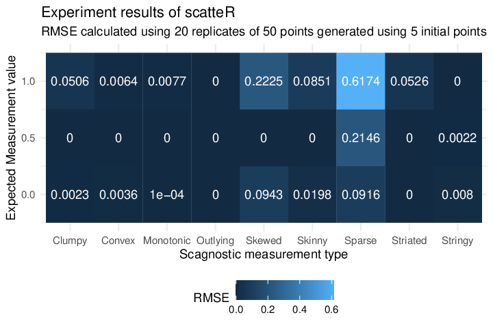
In order to assess the accuracy of this method in generating scatter plots that resemble the scagnostic measurements, an experiment was conducted where each measurement type and value was generated for multiple replicates. The resulting scatterplots were then fed into the scagnostic function to retrieve the generated measurements, which were then used to calculate the Root Mean Square Error (RMSE) as follows.

where $M\in\{\text{Outlying, Skewed,\ldots, Monotonic}\}$ is the measurement type, $V\in\{0.0,0.5,1.0\}$ is the expected measurement value and $R=20$ is the number of replicates performed for the experiment.

The results of the experiment are summarized in Figure 2 where scatteR has been capable of generating scatterplots that on average give scagnostic measurements which are approximately close to the expected scagnostic measurement.

The scatteR algorithm contains an iterative refinement approach where simulated annealing is performed multiple times with increasing sample size and constant parameter size pertaining to the number of initial points. The computation time required to generate a fixed set of points should be studied to measure whether the scatteR algorithm is efficient in providing the samples required. The computational time of scatteR with respect to the different scagnostic measurements and their measurement strengths are presented in Figure 3.

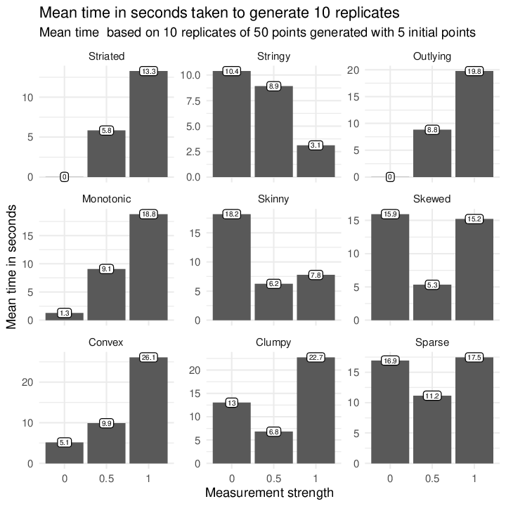
All of the scatteR generations of 50 points using 5 initial points can be completed on average in under 30 seconds. In most cases, the scagnostics with lower strength can be generated quicker than the ones with higher strength. This could be due to the constraints imposed by the scagnostics algorithm, where a perfect 1.0 score in any measurement type would indicate a highly specific scatterplot arrangement.

From the available hyperparameters of the scatteR algorithm, the number of initial points has an impact as it is a deciding factor of the number of parameters that the simulated annealing algorithm has to optimize over in each iteration to make the final scatterplot resemble the expected scagnostics. Therefore, the time consumed by different configurations of the number of initial points was studied and the results are presented in Figure 4.

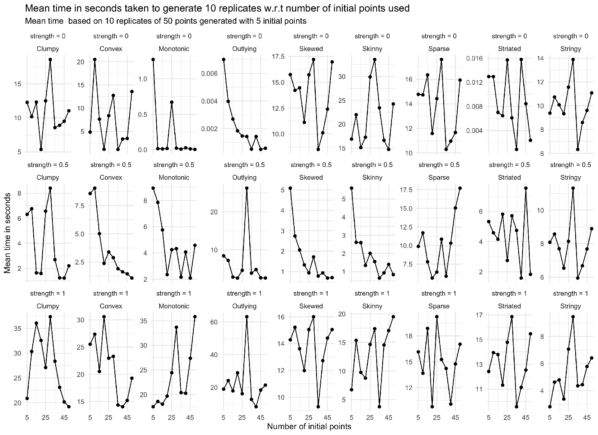
As expected, a higher number of initial points does not increase the computation time. However, there is a spike of time consumed in the range of 25 to 40 initial points utilized.

References

- Arnold et al. (2005) Arnold, K., Gosling, J., and Holmes, D. (2005), The Java programming language, Addison Wesley Professional.
- Conn et al. (2009) Conn, A. R., Scheinberg, K., and Vicente, L. N. (2009), Introduction to derivative-free optimization, SIAM.
- Dang et al. (2012) Dang, T. N., Anand, A., and Wilkinson, L. (2012), “Timeseer: Scagnostics for high-dimensional time series,” IEEE Transactions on Visualization and Computer Graphics, 19, 470–483.
- Dang and Wilkinson (2014a) Dang, T. N. and Wilkinson, L. (2014a), “Scagexplorer: Exploring scatterplots by their scagnostics,” in 2014 IEEE Pacific visualization symposium, IEEE.
- Dang and Wilkinson (2014b) — (2014b), “Transforming scagnostics to reveal hidden features,” IEEE transactions on visualization and computer graphics, 20, 1624–1632.
- Koziel and Yang (2011) Koziel, S. and Yang, X.-S. (2011), Computational optimization, methods and algorithms, volume 356, Springer.
- Lakshika and Talagala (2021) Lakshika, J. P. and Talagala, T. S. (2021), “Computer-aided Interpretable Features for Leaf Image Classification,” arXiv preprint arXiv:2106.08077.
- Pham et al. (2020a) Pham, V., Dang, T., Wilkie, A., and Banterle, F. (2020a), “ScagnosticsJS: Extended Scatterplot Visual Features for the Web.” in Eurographics (Short Papers).
- Pham et al. (2020b) Pham, V., Nguyen, N. V., and Dang, T. (2020b), “Scagcnn: Estimating visual characterizations of 2d scatterplots via convolution neural network,” in Proceedings of the 11th International Conference on Advances in Information Technology.
- R Core Team (2019) R Core Team (2019), R: A Language and Environment for Statistical Computing, R Foundation for Statistical Computing, Vienna, Austria, URL https://www.R-project.org/.
- Simonyan and Zisserman (2014) Simonyan, K. and Zisserman, A. (2014), “Very deep convolutional networks for large-scale image recognition,” arXiv preprint arXiv:1409.1556.
- Sips et al. (2009) Sips, M., Neubert, B., Lewis, J. P., and Hanrahan, P. (2009), “Selecting good views of high-dimensional data using class consistency,” in Computer Graphics Forum, volume 28, Wiley Online Library.
- Srivastava et al. (2019) Srivastava, A., Sharpnack, M., Huang, K., Mallick, P., and Machiraju, R. (2019), “PTR Explorer: An approach to identify and explore Post Transcriptional Regulatory mechanisms using proteogenomics,” in PACIFIC SYMPOSIUM ON BIOCOMPUTING 2020, World Scientific.
- Tsallis and Stariolo (1996) Tsallis, C. and Stariolo, D. A. (1996), “Generalized simulated annealing,” Physica A: Statistical Mechanics and its Applications, 233, 395–406.
- Tukey and Tukey (1985) Tukey, J. W. and Tukey, P. A. (1985), “Computer graphics and exploratory data analysis: An introduction,” in Proceedings of the Sixth Annual Conference and Exposition: Computer Graphics, volume 85.
- Van Rossum and Drake Jr (1995) Van Rossum, G. and Drake Jr, F. L. (1995), Python tutorial, Centrum voor Wiskunde en Informatica Amsterdam, The Netherlands.
- Wang et al. (2019) Wang, Y., Wang, Z., Liu, T., Correll, M., Cheng, Z., Deussen, O., and Sedlmair, M. (2019), “Improving the robustness of scagnostics,” IEEE transactions on visualization and computer graphics, 26, 759–769.
- Wickham (2016) Wickham, H. (2016), ggplot2: Elegant Graphics for Data Analysis, Springer-Verlag New York, URL https://ggplot2.tidyverse.org.
- Wickham et al. (2019) Wickham, H., Averick, M., Bryan, J., Chang, W., McGowan, L. D., François, R., Grolemund, G., Hayes, A., Henry, L., Hester, J., Kuhn, M., Pedersen, T. L., Miller, E., Bache, S. M., Müller, K., Ooms, J., Robinson, D., Seidel, D. P., Spinu, V., Takahashi, K., Vaughan, D., Wilke, C., Woo, K., and Yutani, H. (2019), “Welcome to the tidyverse,” Journal of Open Source Software, 4, 1686.
- Wilkinson and Anand (2018) Wilkinson, L. and Anand, A. (2018), scagnostics: Compute scagnostics - scatterplot diagnostics, URL https://CRAN.R-project.org/package=scagnostics. R package version 0.2-4.1.
- Wilkinson et al. (2005) Wilkinson, L., Anand, A., and Grossman, R. (2005), “Graph-theoretic scagnostics,” in Information Visualization, IEEE Symposium on, IEEE Computer Society.
- Wilkinson and Wills (2008) Wilkinson, L. and Wills, G. (2008), “Scagnostics distributions,” Journal of Computational and Graphical Statistics, 17, 473–491.
- Yang Xiang et al. (2013) Yang Xiang, Gubian, S., Suomela, B., and Hoeng, J. (2013), “Generalized Simulated Annealing for Efficient Global Optimization: the GenSA Package for R.” The R Journal Volume 5/1, June 2013, URL https://journal.r-project.org/archive/2013/RJ-2013-002/index.html.