Macroscopic quantum test with bulk acoustic wave resonators
Abstract
Recently, solid-state mechanical resonators have become a platform for demonstrating non-classical behavior of systems involving a truly macroscopic number of particles. Here, we perform the most macroscopic quantum test in a mechanical resonator to date, which probes the validity of quantum mechanics by ruling out a classical description at the microgram mass scale. This is done by a direct measurement of the Wigner function of a high-overtone bulk acoustic wave resonator mode, monitoring the gradual decay of negativities over tens of microseconds. While the obtained macroscopicity of is on par with state-of-the-art atom interferometers, future improvements of mode geometry and coherence times could test the quantum superposition principle at unprecedented scales and also place more stringent bounds on spontaneous collapse models.
Understanding the quantum-classical transition is one of the main challenges of modern physics. Is the Schrödinger equation valid all the way from the microscopic to the macroscopic world, with quantum effects increasingly hard to observe due to environmental decoherence Schlosshauer 2019? Or do the laws of quantum mechanics break down at some point, so as to reinstate macrorealism in our everyday life Leggett 2002? This question is not philosophical, as it can be tackled by demonstrating genuine quantum effects in ever more macroscopic systems.
Single atoms have been delocalized over macroscopic length and time scales, reaching metres and seconds in state-of-the-art experiments Kovachy et al. 2015; Abend et al. 2016; Asenbaum et al. 2017; Xu et al. 2019. On the other hand, molecule interferometry has pushed the mass boundaries by confirming the wave nature for compounds of more than atomic mass units Eibenberger et al. 2013; Fein et al. 2019. Future Earth- and space-based experiments with freely falling or levitated nanoparticles aim at even higher mass and time scales Stickler et al. 2018; Kaltenbaek et al. 2022, but in such schemes it is a single rigid-body degree of freedom that is placed into a superposition.
This is to be contrasted with growing efforts in electro- and opto-mechanics toward demonstrating quantum states in the elastic deformation of condensed matter systems of substantially higher mass. Recent experimental milestones include the successful preparation of nonclassical states of surface and bulk acoustic modes, demonstrated through the observation of Wigner function negativities Chu et al. 2018; Satzinger et al. 2018; Wollack et al. 2022; von Lüpke et al. 2022; Bild et al. 2022. Such nonclassical states of motion involve a truly macroscopic number of atoms, on the order of , vibrating in unison. At the same time, each atom is delocalized only over a tiny fraction of the size of an atomic nucleus, which makes unclear how they compare to previous tests of the quantum-classical transition.
Using an objective measure for the degree of macroscopicity of nonclassical states Nimmrichter and Hornberger 2013, we report here the most macroscopic quantum test performed with a solid-state mechanical resonator. The macroscopicity value obtained in our experiment is surprisingly large, motivating us to optimize the design specifications for future electromechanical experiments to become competitive even with matter-wave superposition tests.

To justify the macroscopicity measure used, note that any genuine quantum test probes the validity of quantum mechanics against the hypothesis of macrorealism: that a modification of quantum theory destroys coherence above a certain size or mass scale, rendering superposition phenomena unobservable in practice. Hence, the degree to which a quantum experiment falsifies a broad, generic class of minimally invasive, macrorealistic modifications of quantum mechanics gives rise to an objective benchmark Nimmrichter and Hornberger 2013: Using the measurement data to rule out a range of values of the coherence time parameter quantifying the macrorealist modification, an experiment is justifiably the more macroscopic the greater the -values falsified through Bayesian inference Schrinski et al. 2019. The macroscopicity measure is then determined by the logarithm of the greatest ruled out -value 11 1 Note that the macrorealist modification hypothesis can be probed also in experiments that to do not involve quantum superpositons. Only observations of genuine quantum signatures can therefore be assigned a benchmark value Schrinski et al. 2019. This requires the interrogated state not to have an underlying classical description, excluding all oscillator states with positive Wigner function.. To date, the highest macroscopicity has been achieved in molecule interferometry Fein et al. 2019.
In our experiment, we observe Wigner function negativities for up to s in an bulk acoustic vibration mode of a sapphire crystal with an effective mass of g, which is prepared in a single-phonon state and in a superposition of Fock states. This quantum signature is detected by measuring the displaced parity Royer 1977 of the quantum state using a superconducting qubit, see Fig. 1. Our analysis shows that it can be associated with a large macroscopicity , despite the sub-nuclear delocalization of the atoms involved. Based on this, we explain how future experiments with bulk acoustic resonators may realize the most macroscopic quantum test.

Macroscopicity of bulk resonator modes.– To evaluate the macroscopicity of a demonstrated quantum effect, one should consider the class of macrorealistic models possibly falsified by the experiment. Keeping those models minimally invasive in that they preserve linearity, the semigroup nature of the time evolution, invariance under the chosen non-relativistic reference frame, and other basic consistency principles Nimmrichter and Hornberger 2013, their observable impact can be formulated as a Lindblad generator modifying the quantum evolution of the system state . For a large compound of atomic constituents with masses , the generator reduces to Nimmrichter and Hornberger 2013
| (1) |
with . The strength of the modification is specified by the coherence time parameter and the standard deviation of the isotropic Gaussian momentum distribution . The Lindblad operators are mass-weighted sums of single-particle momentum kicks by , , with the particle position operators and a reference mass chosen to be that of an electron.
We note that the theory of continuous spontaneous collapse (CSL) can be described by (1), but it is usually parameterized in terms of a rate per atomic mass unit , and a localisation length Bassi et al. 2013. The strongest bounds on these CSL parameters are currently achieved by so-called non-interferometric tests Carlesso et al. 2022, where one measures the noise experienced by a classical system by exploiting the fact that macrorealistic modifications are accompanied by a heating effect. However, a genuine quantum signal, such as interference fringes or a negative Wigner function, is required for a CSL test to also probe the validity of quantum mechanics in the system.
In the following, we consider a collective acoustic excitation in the bulk condensed matter, taking the form
| (2) |
of waist , mode index , and length . (The mode vanishes for , and is laterally well confined within the material.) The effective volume of the mode is defined as and, given the mass density , the effective mass is defined as . This way one consistently obtains the total bulk volume and mass in the limiting case of a center of mass motion, corresponding to a uniform displacement with , so that can be understood as the mass fraction taking part in the displacement Sup.
The mode is quantized by means of the ladder operator , involving a conjugate pair of dimensionless position and momentum quadrature operators, . A single phononic excitation thus displaces the atoms by amplitudes of the order of the zero-point fluctuation , with , around their equilibrium positions according to the mode displacement field, i.e. . The Lindblad operators thus become
| (3) |
In the relevant regime of modification length scales larger than the interatomic distances, it is safe to assume a homogeneous mass density and to expand the operator in (3) to first order in Schrinski et al. 2019. This results in momentum diffusion, , with a diffusion rate amplified by the effective oscillator mass,
| (4) |
The rate depends on how the modification length scale compares to the geometric length scales of the oscillator mode, as determined by , , , and . The integral can be given analytically, leading to a lengthy expression for . In the limit and for even, we find , whereas for and , we get . The maximum with respect to is located in between at , provided that and Sup,
| (5) |
Given a fixed sound velocity , and noting , the maximum rate value is proportional to the square of the mode wavelength .
In the co-rotating frame of the oscillator, and including energy decay at rate , the modified time evolution of the oscillator state is given by the master equation
| (6) |
In the second line we average over the rapidly oscillating cross-terms, as we are interested in decoherence on time scales much longer than the oscillation period.
The coarse-grained isotropic master equation (6) admits a compact solution in the Wigner function representation
| (7) |
with . This expression can be computed analytically for several states of interest, such as Fock states and their superposition Sup. Bayesian parameter estimation based upon Eq. (Macroscopic quantum test with bulk acoustic wave resonators) allows us to identify from the measured Wigner functions the threshold value that corresponds to the most conservative quantile of the coherence time at any Sup; Schrinski et al. 2019. Greater are also compatible with the data, as the observed decoherence might as well be due to unspecified conventional noise sources, but smaller times can be ruled out with confidence. Macroscopicity is then defined as follows: We convert into the corresponding macrorealistic coherence time parameter by virtue of (4), maximize over to obtain the greatest excluded , and assign a macroscopicity value .
By modelling the state evolution with (6), we thus assume a zero-temperature environment and attribute any heating or decoherence beyond energy relaxation at the rate to the impact of a macrorealistic modification described by infinite-temperature diffusion at the rate . This amounts to a conservative assessment of the macroscopicity, since, by overestimating the hypothetical contribution of macrorealistic diffusion to the observed decoherence, we overestimate and thus underestimate . We characterise the energy relaxation rate independently, by a standard measurement of the phonon decay time and the steady-state population Sup.
Experiment.– Our measurements are carried out on a high-overtone bulk-acoustic wave resonator (HBAR) device cooled down at millikelvin temperature, see Fig. 1, which makes use of a superconducting qubit to prepare, control, and read-out the quantum excitation of a mechanical mode localized in the bulk of a sapphire substrate von Lüpke et al. 2022.
The acoustic vibration mode is described to a very good approximation by Eq. (2), as also verified by numerical simulations. It oscillates over the bulk length at angular frequency with wavelength , corresponding to the mode index . Assuming a homogenous mass density g/cm3, and given the transverse waist , we obtain the effective oscillator mass g and a zero-point fluctuation of . For these parameters, we find from Eq. (4) a maximal diffusion rate of at a critical length scale m, which is of the same order as the mode wavelength.
The coherence properties of the phonon mode are characterized by a small one-phonon steady-state population of , by the relaxation time s, and by the Ramsey dephasing time s Sup. These imply a much longer pure dephasing time of . Relaxation, which originates from the coupling to the environment through e.g. surface scattering or diffraction loss, thus dominates the degradation of quantum features over time, and we can safely assume within error tolerance.
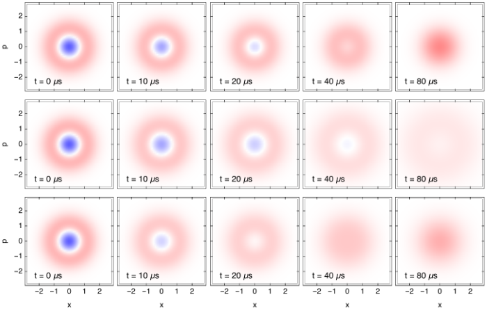
Using the toolbox of circuit quantum acoustodynamics (cQAD), we can use the qubit to prepare and measure the HBAR in nonclassical states of motion Chu et al. 2018. In particular, an arbitrary superposition with the first excited state, , can be prepared by swapping the qubit state to the mechanical mode through the resonant Jaynes–Cummings interaction. For any we obtain a nonclassical state of motion with negativities in the Wigner function, that will degrade over time due to relaxation. To monitor this effect, we let the system evolve for a time , and then obtain the Wigner function of the mechanical state by measuring its displaced parity von Lüpke et al. 2022; Sup. Fig. (2) shows how the measured Wigner function degrades over time for an initial Fock state (top row) and an initial superposition state (bottom row). Note the disappearance of negative (blue) regions in the quasi-probability distribution, turning it into a classical phase-space distribution.
In the first part of the experiment, we prepare the resonator in the single-phonon Fock state and measure its Wigner quasi-probability distribution as a function of time (Fig. 2, top row). We observe that the region of negative values around the phase space origin shrinks gradually, persisting for tens of microseconds, before the Wigner function turns purely positive and becomes indistinguishable from a classical distribution. The longer and more pronounced the initial negativity remains, the stronger the experiment falsifies macrorealist modifications of quantum mechanics. We estimate the impact of such modifications by first fitting the initial measurement at with the Wigner function of an incoherent mixture of and , thus accounting for imperfections in the state preparation and measurement. The measured Wigner functions at 10 s, 20 s, and 40 s are then compared to the theoretical expectation (Macroscopic quantum test with bulk acoustic wave resonators) including energy relaxation with the measured rate as well as modification-induced diffusion with variable rate . Bayesian parameter estimation and subsequent maximization with respect to shows that any can be excluded with 95 confidence (at ) Sup. This corresponds to a macroscopicity of , by far the highest value reported on mechanical resonators, see Tab. I. We note that the obtained diffusion rate is consistent with what is found by using our system to perform a so-called non-interferometric test of macrorealistic models based on the observed residual excitation of the mode Sup. Thus our analytic results can be straightforwardly adopted in such schemes, as recently proposed in Ref. Tobar et al. 2022.
In the second part of the experiment, we prepare the resonator in the superposition state . As shown in the bottom row of Fig. 2, the measured Wigner function again takes negative values, confirming the nonclassicality of the initial state. The asymmetry around the origin, whose phase can be controlled by the qubit state, rotates due to a small detuning between the oscillator and the displacement pulse frequencies. This rotation is accounted for in our data processing. Following the previous analysis, we find that the superposition state data is compatible with a maximal diffusion rate of , which is a factor of four larger than the rate found from the Fock state and from the non-interferometric test Sup. This discrepancy can be explained by the presence of an additional pure dephasing channel with a rate of . While circularly symmetric Wigner functions such as single Fock states are unaffected by this decoherence channel, which corresponds to a random rotation around the phase-space origin, a superposition of Fock states, which is necessarily asymmetric, gets washed out at rate , removing any negativity. However, to fairly assess the macroscopicity of the Fock state superposition, we do not include this decoherence channel into the master equation (6), so that all decoherence is attributed to the macrorealistic modification. This results in a greater diffusion rate, and consequently in a lower macroscopicity of . If we included the dephasing effect in the Bayesian inference the resulting rate would be consistent with both the Fock state analysis and the non-interferometric test.
Beating the macroscopicity record.–Based on our experimental results, and using the analytical result (4), we can now establish how to optimize future quantum experiments with bulk acoustic resonators to become competitive with the most macroscopic quantum tests to date. In contrast to quantum tests based on the interference of center-of-mass degrees of freedom, the diffusion rate scales here only weakly with the mass and length scales of the material: in the realistic case of comparable lateral and longitudinal mode extension (), we find that macrorealistic diffusion is strongest at a length scale comparable to the mode wavelength . To attain greater macroscopicity in a given material, one should strive to increase the mode wavelength since the maximum diffusion rate (5) grows like . Apart from these geometric considerations, the macroscopicity also benefits from longer relaxation and coherence times , and a better characterization of the measurement noise. The latter can be incorporated into the Bayesian parameter estimation to extract better bounds, instead of adding a broad Gaussian noise channel as done in the analysis above.
As an example, keeping the same device and mode geometry as in the present experiment, but using a mode with and , would result in , surpassing all reported quantum tests, see Tab. I. We obtain this estimate by setting and rescaling the observed coherence time in proportion to ; the macroscopicity grows logarithmically with increasing coherence time. Beyond that, out-of-plane drum modes with frequencies in the low MHz range and huge quality factors have been reported, corresponding to Seis et al. 2022. If genuine quantum effects could be demonstrated in these devices, they might reach substantially greater macroscopicities 22 2 This rough estimate is based on Schrinski et al. 2019, by approximating the mode in Seis et al. 2022 as the fundamental Bessel mode , for a disc with diameter m, nm thickness, and pg. Precise -values would depend on a combination of effective mass, mode profile, and observed duration of Wigner negativities..
| experiment | year | ||
|---|---|---|---|
| mechanical resonators | Bulk acoustic waves [this work] | 2022 | 11.3 |
| Phononic crystal resonator Wollack et al. 2022 | 2022 | ||
| Surface acoustic waves Satzinger et al. 2018 | 2018 | ||
| matter-wave interference | Molecule interferometry Fein et al. 2019 | 2019 | 14.0 |
| Atom interferometry Xu et al. 2019 | 2019 | 11.8 | |
| BEC interferometry Asenbaum et al. 2017 | 2017 | 12.4 |
Conclusion.–We demonstrated the most macroscopic quantum test with bulk acoustic wave resonators, based on monitoring the time evolution of nonclassical Wigner functions. The reported macroscopicity is comparable to the one obtained by an experiment holding cesium atoms in a spatial superposition at separation over 20 seconds Xu et al. 2019. In the future, we envisage improved resonator designs that may surpass the most macroscopic matter wave interferometers, testing the validity of quantum mechanics at unprecedented scales.
Acknowledgements.– We would like to thank Georg Enzian and Eric Planz for helpful discussions. BS was supported by Deutsche Forschungsgemeinschaft (DFG, German Research Foundation), Grant No. 449674892. UvL is funded by the SNF project number 200021_204073. MF was supported by The Branco Weiss Fellowship – Society in Science, administered by the ETH Zürich.
References
- Schlosshauer (2019) M. Schlosshauer, Quantum decoherence, Phys. Rep. 831, 1 (2019).
- Leggett (2002) A. J. Leggett, Testing the limits of quantum mechanics: motivation, state of play, prospects, J. Phys.: Condens. Matter 14, R415 (2002).
- Kovachy et al. (2015) T. Kovachy, P. Asenbaum, C. Overstreet, C. A. Donnelly, S. M. Dickerson, A. Sugarbaker, J. M. Hogan, and M. A. Kasevich, Quantum superposition at the half-metre scale, Nature 528, 530 (2015).
- Abend et al. (2016) S. Abend, M. Gebbe, M. Gersemann, H. Ahlers, H. Müntinga, E. Giese, N. Gaaloul, C. Schubert, C. Lämmerzahl, W. Ertmer, W. P. Schleich, and E. M. Rasel, Atom-chip fountain gravimeter, Phys. Rev. Lett. 117, 203003 (2016).
- Asenbaum et al. (2017) P. Asenbaum, C. Overstreet, T. Kovachy, D. D. Brown, J. M. Hogan, and M. A. Kasevich, Phase shift in an atom interferometer due to spacetime curvature across its wave function, Phys. Rev. Lett. 118, 183602 (2017).
- Xu et al. (2019) V. Xu, M. Jaffe, C. D. Panda, S. L. Kristensen, L. W. Clark, and H. Müller, Probing gravity by holding atoms for 20 seconds, Science 366, 745 (2019).
- Eibenberger et al. (2013) S. Eibenberger, S. Gerlich, M. Arndt, M. Mayor, and J. Tüxen, Matter–wave interference of particles selected from a molecular library with masses exceeding 10000 amu, Phys. Chem. Chem. Phys. 15, 14696 (2013).
- Fein et al. (2019) Y. Y. Fein, P. Geyer, P. Zwick, F. Kiałka, S. Pedalino, M. Mayor, S. Gerlich, and M. Arndt, Quantum superposition of molecules beyond 25 kda, Nat. Phys. 15, 1242 (2019).
- Stickler et al. (2018) B. A. Stickler, B. Papendell, S. Kuhn, B. Schrinski, J. Millen, M. Arndt, and K. Hornberger, Probing macroscopic quantum superpositions with nanorotors, New J. Phys. 20, 122001 (2018).
- Kaltenbaek et al. (2022) R. Kaltenbaek et al., Research campaign: Macroscopic quantum resonators (MAQRO), Quantum Sci. Technol. 10.1088/2058-9565/aca3cd (2022).
- Chu et al. (2018) Y. Chu, P. Kharel, T. Yoon, L. Frunzio, P. T. Rakich, and R. J. Schoelkopf, Creation and control of multi-phonon Fock states in a bulk acoustic-wave resonator, Nature 563, 666 (2018).
- Satzinger et al. (2018) K. J. Satzinger, Y. P. Zhong, H. S. Chang, G. A. Peairs, A. Bienfait, M.-H. Chou, A. Y. Cleland, C. R. Conner, É. Dumur, J. Grebel, I. Gutierrez, B. H. November, R. G. Povey, S. J. Whiteley, D. D. Awschalom, D. I. Schuster, and A. N. Cleland, Quantum control of surface acoustic-wave phonons, Nature 563, 661 (2018).
- Wollack et al. (2022) E. A. Wollack, A. Y. Cleland, R. G. Gruenke, Z. Wang, P. Arrangoiz-Arriola, and A. H. Safavi-Naeini, Quantum state preparation and tomography of entangled mechanical resonators, Nature 604, 463 (2022).
- von Lüpke et al. (2022) U. von Lüpke, Y. Yang, M. Bild, L. Michaud, M. Fadel, and Y. Chu, Parity measurement in the strong dispersive regime of circuit quantum acoustodynamics, Nat. Phys. 18, 794 (2022).
- Bild et al. (2022) M. Bild, M. Fadel, Y. Yang, U. von Lüpke, P. Martin, A. Bruno, and Y. Chu, Schrödinger cat states of a 16-microgram mechanical oscillator, arXiv preprint arXiv:2211.00449 (2022).
- Nimmrichter and Hornberger (2013) S. Nimmrichter and K. Hornberger, Macroscopicity of mechanical quantum superposition states, Phys. Rev. Lett. 110, 160403 (2013).
- Schrinski et al. (2019) B. Schrinski, S. Nimmrichter, B. A. Stickler, and K. Hornberger, Macroscopicity of quantum mechanical superposition tests via hypothesis falsification, Phys. Rev. A 100, 032111 (2019).
- (18) Note that the macrorealist modification hypothesis can be probed also in experiments that to do not involve quantum superpositons. Only observations of genuine quantum signatures can therefore be assigned a benchmark value Schrinski et al. 2019. This requires the interrogated state not to have an underlying classical description, excluding all oscillator states with positive Wigner function.
- Royer (1977) A. Royer, Wigner function as the expectation value of a parity operator, Phys. Rev. A 15, 449 (1977).
- Bassi et al. (2013) A. Bassi, K. Lochan, S. Satin, T. P. Singh, and H. Ulbricht, Models of wave-function collapse, underlying theories, and experimental tests, Rev. Mod. Phys. 85, 471 (2013).
- Carlesso et al. (2022) M. Carlesso, S. Donadi, L. Ferialdi, M. Paternostro, H. Ulbricht, and A. Bassi, Present status and future challenges of non-interferometric tests of collapse models, Nat. Phys. 18, 243 (2022).
- (22) See Supplementary Information for details on the experimental setup and the theoretical calculations, including Refs. Jeffreys 1946; Arrangoiz-Arriola 2019; Satzinger 2018; Satzinger; Chu et al. 2017; Armano et al. 2016; Carlesso et al. 2016.
- Tobar et al. (2022) G. Tobar, S. Forstner, A. Federov, and W. P. Bowen, Testing spontaneous wavefunction collapse with quantum electromechanics, arXiv preprint arXiv:2206.14531 (2022).
- Seis et al. (2022) Y. Seis, T. Capelle, E. Langman, S. Saarinen, E. Planz, and A. Schliesser, Ground state cooling of an ultracoherent electromechanical system, Nat. Comm. 13, 1507 (2022).
- (25) This rough estimate is based on Schrinski et al. 2019, by approximating the mode in Seis et al. 2022 as the fundamental Bessel mode , for a disc with diameter m, nm thickness, and pg. Precise -values would depend on a combination of effective mass, mode profile, and observed duration of Wigner negativities.
- Schrinski et al. (2020) B. Schrinski, S. Nimmrichter, and K. Hornberger, Quantum-classical hypothesis tests in macroscopic matter-wave interferometry, Phys. Rev. Res. 2, 033034 (2020).
- Jeffreys (1946) H. Jeffreys, An invariant form for the prior probability in estimation problems, Proc. R. Soc. Lond. A 186, 453 (1946).
- Arrangoiz-Arriola (2019) P. Arrangoiz-Arriola, Quantum acoustics with lithium niobate nanostructures, Ph.D. thesis, Stanford University (2019).
- Satzinger (2018) K. J. Satzinger, Quantum control of surface acoustic wave phonons, Ph.D. thesis, UC Santa Barbara (2018).
- (30) K. J. Satzinger, private communication.
- Chu et al. (2017) Y. Chu, P. Kharel, W. H. Renninger, L. D. Burkhart, L. Frunzio, P. T. Rakich, and R. J. Schoelkopf, Quantum acoustics with superconducting qubits, Science 358, 199 (2017).
- Armano et al. (2016) M. Armano, H. Audley, G. Auger, J. Baird, M. Bassan, P. Binetruy, M. Born, D. Bortoluzzi, N. Brandt, M. Caleno, et al., Sub-femto-g free fall for space-based gravitational wave observatories: Lisa pathfinder results, Phys. Rev. Lett. 116, 231101 (2016).
- Carlesso et al. (2016) M. Carlesso, A. Bassi, P. Falferi, and A. Vinante, Experimental bounds on collapse models from gravitational wave detectors, Phys. Rev. D 94, 124036 (2016).
Supplementary information
Supplementary Section A Geometric factor
The considered macrorealistic modifications lead to momentum diffusion in the oscillator state. The momentum diffusion rate is inversely proportional to the coherence time parameter and depends on the oscillator mode function through the geometric factor Schrinski et al. 2019
| (8) |
Here, denotes the reference electron mass, and a Gaussian momentum distribution of standard deviation . The resonator mode employed in this work can be modelled to great accuracy with the function
| (9) |
where is the beam waist ( amplitude radius), is the height, and the mode index. Based on this mode function, we can define an effective mode volume and mass, and . They both depend on the square of the amplitude prefactor , but the relevant physical displacement amplitudes of the individual atoms, , as well as the dimensionless macrorealistic diffusion rate, , do not depend on . Hence we may set , without loss of generality, as done in the main text.
Given that we consider a displacement field with only a longitudinal component in -direction, , and that the mass density distribution is assumed to be uniform (i.e. ), Eq. (8) can be simplified further:
| (10) |
This allows us to first integrate out the momenta , change to cylindrical coordinates and express the end result as
| (11) |
with and . Once we identify , we arrive at the expression for the diffusion rate given in the main text. A non-tight upper bound follows by pulling the absolute value into the -integral in (11). The -integral then evaluates to , so that , and . The scaling of this bound with the mode mass and geometry is deceivingly similar to previous results for center-of-mass oscillations. However, we will see in the following that the bound is rather loose and the actual diffusion rate for bulk acoustic modes exhibits a completely different scaling.
In the limiting case , the Gaussian function is sharply peaked around , and we can expand the remainder of the integrand to lowest non-vanishing order; for even , this yields , and . For decreasing , this rate drops as . Notice that odd would result in a -scaling, .
Greater care must be taken in the opposite limit, . Although the non-Gaussian part of the integrand in (11) is clearly peaked around , it is asymptotically of order and thus non-integrable without the regularizing presence of the Gaussian. Hence a dominant contribution to the -integral in (11) does not come from the vicinity of the peaks, but from . For even greater values , we can approximate to lowest order
| (12) |
The corresponding diffusion rate reads as , which does not depend on , is proportional to , and is again monotonic in . In order to access the most relevant intermediate -regime of maximum diffusion, consider the correction , which can be expressed as
| (13) |
The non-Gaussian part of this integrand (square-bracketed) is not only sharply peaked at , but also asymptotically converges to zero like . The integral of this expression evaluates to . Assuming , we can now replace in the Gaussian by , so that
| (14) |
Presuming , the local maximum of coincides approximately with that of , at . It marks the -value at which the experiment is most sensitive to macrorealistic diffusion. The maximum rate reads as
| (15) |
For numerical evaluation, an exact expression of the diffusion rate can be given in terms of
| (16) |
The function can be evaluated to
| (17) |
where
| (18) |
In Fig. S3, we plot the resulting diffusion rate as a function of the modification parameter . We compare the mode addressed in our experiment to one with a much lower frequency and mode index. Based on the above reasoning, the maxima are expected to be at m () and m (), which roughly agrees with the exact positions on the logarithmic scale. The dotted line represents from (14), a good approximation in the relevant regime around maximum diffusion. The dashed lines show the asymptotic approximations for (left) and for (right).
Supplementary Section B Initial states and time evolution
In our setup, macrorealistic collapse models are put to the test by monitoring the decay of Fock and superposition states over a finite amount of time. To assess the influence of those models, it is convenient to solve the time evolution in the Wigner phase space representation of the oscillator state. The one-dimensional Wigner function is defined as
| (19) |
where and are the position and momentum coordinates of the harmonic oscillator. For better readability we now change to dimensionless units and . Then the Wigner functions (19) of the ground state , first exited Fock state , and the superposition state , respectively, read as
| (20) |
The time evolution of the state described by the master equation (6) in the main text describes the impact of the macrorealistic diffusion at the rate , averaged over the free oscillation, and it includes also an environmental decay channel at the rate . The two separate Lindblad generators for decay and amplification, and with , translate into phase space as
| (21) | ||||
| (22) |
Both are classical Fokker-Planck equations, and the first one describes thermalization at the (dimensionless) energy , i.e. the ground state energy of the quantum oscillator. The master equation then yields
| (23) |
The solution to this Fokker-Planck equation is obtained with help of a Fourier transform into the characteristic function representation,
| (24) |
which evolves according to
| (25) |
We can now separate the simple relaxation dynamics (an exponential contraction toward the origin) from the diffusion. Let , , and , which then obeys
| (26) | ||||
| as solved by | ||||
| (27) | ||||
| so that | ||||
| (28) | ||||
From this expression it is evident that the time evolution of an initial is simply given by a multiplication with a Gaussian exponential combined with an isotropic rescaling of the arguments. Noting that at any time, one can check that the asymptotic steady state is a Gaussian, , which for is the ground state of the harmonic oscillator.
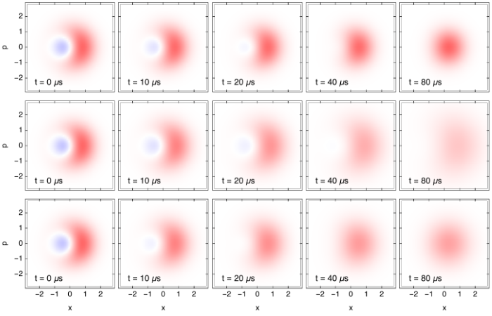
Back in the Wigner representation, the solution turns into a rescaling combined with a Gaussian convolution. Introducing the dimensionless quantitiy , we get
| (29) |
The two last lines are alternative ways to write the convolution. Given the simple Gaussian form of the initial Wigner functions (20), the integrals can be calculated analytically and result in
| (30) | ||||
| (31) | ||||
| (32) |
with . These expressions can be directly compared to the experimentally reconstructed Wigner function, which allows us to perform Bayesian parameter estimation of the macrorealistic -values that are compatible with the measured data.
In Fig. S4, we use Eqs. (31), (32) to illustrate the evolution of states and according to either pure relaxation, pure diffusion, or a combination of both. Notice the significant differences in the dynamics between the different cases.
Supplementary Section C Bayesian parameter estimation
By measuring the Wigner function at several instances of time and comparing it to the theoretical predictions in Sect. B, one can infer the most likely values for the macrorealistic diffusion rate and, subsequently, for the values of the time parameter by virtue of Bayes’ rule. The posterior distribution of -values given the measured data , a fixed value of the parameter , and an independently inferred decay time , updates as Schrinski et al. 2019
| (33) |
Here, subsumes all recorded pixel values of the two-dimensional Wigner function reconstructions at the times , as plotted in the main text. The likelihood for follows from the theoretical model for the Wigner function evaluated at the recorded pixel coordinates and times, , and the assumption of additional Gaussian noise in each data point. That is, we model the likelihood for each pixel value by a Gaussian distribution of standard deviation , so that
| (34) |
We extract the overall noise level by taking a sample of all pixel values for the Fock- measurements at and subtracting the respective model Wigner functions with decay time and without macrorealistic diffusion (). A histogram of the resulting pixel deviations is shown in Fig. S5(a), together with a Gaussian fit that yields the noise level .
The prior is chosen as Jeffreys’ prior Jeffreys 1946, which is maximally objective and fair in a comparison with other completely different experiments Schrinski et al. 2019. It is defined as
| (35) |
where is the Fisher information of the likelihood with respect to and denotes the expectation value over all possible measurement results, .
We perform the Bayesian update (33) with the data obtained for the three time snapshots at . Figures S5(b) and (c) show the resulting posterior distributions over -values for the Fock- and the superposition state, respectively. The upper five-percent quantiles for , marked by vertical lines, correspond to lower five-percent quantiles of at a given value for . Smaller time parameters are thus ruled out with 95% confidence. We find the threshold values of and in (b) and (c), respectively. More conservatively, the respective bounds would be and at the confidence level (roughly corresponding to for normally distributed estimates), or and at the confidence level (roughly ). We attribute the greater threshold value in the superposition measurement to the omitted influence of environmental dephasing, which occurs at a comparable rate of , as discussed in the main text. The remaining discrepancy between this rate and the inferred can be explained by the different impact of diffusion and pure dephasing on the oscillator state.
In order to obtain the macroscopicity values, we take the maximum of the ruled out -range over , which coincides with the local maximum of the dimensionless diffusion rate at , as depicted in Fig. S3. Employing the same 95% confidence level as in previous assessments, this leads to the macroscopicity values and for the two measured states.
Supplementary Section D Macroscopicity estimates for other mechanical resonators
We report here the parameters used to estimate the macroscopicities reachable in the two other reported experiments with mechanical resonators, where Wigner function negativities have been measured in the initial state Satzinger et al. 2018; Wollack et al. 2022. These experiments involve resonators with acoustic modes of complicated geometry Arrangoiz-Arriola 2019; Satzinger 2018, so that it is not easy to derive simple analytical expressions as for the Laguerre-Gaussian modes we considered. For this reason, we proceed with making a conservative analysis, based on approximating such devices to cuboids hosting a sinusoidal displacement field, with the longitudinal extension of the mode. This yields an analytic expression for the geometric factor (8) determining macrorealistic diffusion, which would otherwise require numerical integration of the displacement field resulting from a finite-element simulation of the actual device. Our approximation is conservative in the sense that it likely overestimates the effective oscillator mass, but we do not expect it to result in macroscopicities that deviate much from the actual one (given that is in logarithmic scale).
The experiments in Refs. Satzinger et al. 2018; Wollack et al. 2022 show measurements of Wigner function negativities with the sake of demonstrating nonclassical state preparation, but they do not monitor the disappearance of such quantum features with time. We can therefore merely estimate the potential of these setups to perform a test of macrorealist models from the limitations imposed by the reported -times. To this end, we simply assume that our data were obtained with their resonators at the same relative times , which amounts to rescaling our inferred -values by the ratio between our time and theirs.
Phononic crystal resonator Ref. Wollack et al. 2022: We consider a phonon mode with frequency , wavelength , and decay time . The resonator itself is approximated by a lithium niobate (density ) cuboid of size and total mass , with an effective mass of . We assume a hypothetical experiment that excludes diffusion rates , which results in after maximizing with respect to .
Surface acoustic waves Ref. Satzinger et al. 2018: We consider a phonon mode with frequency , wavelength , and decay time . The resonator is approximated by a lithium niobate (density ) cuboid of size Satzinger , with total mass and effective mass . The hypothetical experiment would exclude , resulting in .
Supplementary Section E Experimental sequences
E.1 Phonon mode characterization
To characterize the phonon mode under investigation, we perform two standard measurements Chu et al. 2017. The first is a population decay (“ring-down”) measurement, which gives the relaxation rate . This is done by preparing the phonon mode in Fock state , and then monitoring its population decay over time, see Fig. (S6). Fitting the measured data with a decaying exponential plus a constant background gives us the time parameter , where the error is one standard deviation given by the fitting function. In the assumed model (6), the measured relaxation rate corresponds to .
The second measurement consists of a Ramsey sequence, which monitors dephasing effects. This is done by preparing the phonon mode in state , and then monitoring its phase evolution over time, see Fig. (S6). Fitting the measured data to an exponentially decaying oscillation gives us the time constant , where the error is one standard deviation given by the fitting function. As this contrast reduction is partially due to the relaxation effect previously investigated, it is convenient to identify the pure dephasing time as . This pure dephasing could be described by a Lindblad generator of the form .
We can also estimate the ground state population and the effective temperature of the phonon mode, which can be used for a classical noise test of macrorealistic collapse models. To this end, we tune the qubit frequency to be below the one of the phonon mode, operating our system in the strongly dispersive regime von Lüpke et al. 2022. In this regime, the qubit frequency depends on the phonon mode occupation number, and therefore on its effective temperature. In Fig. S7 we present a spectroscopic measurement of the qubit frequency with the phonon mode in the stationary state, showing a prominent peak at the bare qubit frequency. From the data it is possible to note a slight asymmetry between the left and right tails of the peak, which is highlighted by comparing to a Voigt profile fit (blue line). This is expected at finite temperature, as any population in higher Fock states will result in additional peaks on the left-hand side of the main one. As the position of the peak for is known, we fit again the data with a sum of two Voigt profiles of fixed frequencies (red dashed line). From the relative amplitude between the two peaks we estimate the thermal population of the 1-phonon excited state to be . In our model (6) in the main text, this small population corresponds to to a good approximation. Hence , and we can safely identify the measured relaxation rate with the model rate, , within the uncertainty of the fit.
E.2 State preparation and read-out
To acquire the data presented in Fig. 2 of the main text, we adopt the sequence illustrated in Fig. S8. First, the phonon mode is prepared in state or by swapping the corresponding qubit states or with the phonon ground state through the resonant Jaynes–Cummings interaction. Then, the system evolves freely for a variable time interval , after which a Wigner function measurement is performed. The latter consists of a displaced parity measurement, where a displacement of the phonon mode is followed by a parity measurement implemented through a strong dispersive interaction between the qubit and the phonon von Lüpke et al. 2022.
The above sequence results in a single measurement of the parity at point in phase space. The value of the Wigner function is then obtained by averaging of such parity measurements. Finally, to record a two-dimensional Wigner function like the ones in Fig. 2, we repeat the described procedure for many different values of .

Supplementary Section F Non-interferometric thermalization test
A straightforward and widely used approach to study collapse models are so-called non-interferometric tests, which focus on monitoring the noise or the energy changes in the studied system Carlesso et al. 2022. This puts bounds on modifications to quantum mechanics without the need of preparing a quantum state. In our experiment, we can do a similar analysis by monitoring the resonator occupation number. The Wigner function evolution under relaxation at the rate and macrorealistic diffusion predicts a steady-state energy . Hence, by measuring the steady state phonon population, we impose bounds on the hypothetical diffusion rate .
To improve the bounds resulting from this analysis, one could also take into account additional known decoherence processes and a finite temperature characterized from independent measurements. Instead, we follow the most conservative estimation: we attribute all diffusion effects to the macrorealistic modification, thus overestimating its effect and underestimating the resulting bounds. Then the equilibrium temperature is a result of the competing relaxation rate and macrorealistic diffusion rate . The decay rate can be reliably measured far from equilibrium by preparing a thermal state at and verifying a constant decay rate. This leaves only one free parameter to estimate, which then gives non-interferometric exclusion bounds on collapse models based on the observed amount of classical heating.
With the maximum dimensionless diffusion rate and a thermal population of , this analysis leads to . The measured then results in an exclusion of s at the length scale m. This is weaker than other non-interferometric collapse tests performed with ad hoc experiments Carlesso et al. 2022, or with large-scale endeavors like the LISA pathfinder experiment Armano et al. 2016; Carlesso et al. 2016, but it could be further improved by carefully optimizing the HBAR device geometry and the experimental sequences. Note however that no genuine quantum feature is actually verified in a collapse test based on classical noise bounds, meaning that it does not qualify for a benchmark based on the macroscopicity of a superposition.
Finally, as a side remark, let us mention that a new approach for performing non-interferometric tests of collapse models using bulk resonators has been recently proposed in Ref. Tobar et al. 2022. Our analytical results can readily be applied to this proposal, leading to an exact expression of the diffusion rate. Given the mode function hosted by a homogeneous cylinder of radius and length , we obtain the diffusion rate
| (36) |
For convenience, we have adopted the parameter notation of the CSL collapse model here, and . Our formula must be multiplied by two for direct comparison with the approximate momentum diffusion rate term given by the authors,
| (37) |
A comparison between both expressions is shown in Fig. S9 for the parameters chosen in Ref. Tobar et al. 2022, , , , and for the two settings at and at , showing good agreement.