Sufficient Conditions for Persistency of Excitation with Step and ReLU Activation Functions

Let $\phi:\mathbb{R}^{n}\to\mathbb{R}^{N}$ be a vector function defined as

where $\phi_{1},\dots,\phi_{N}:\mathbb{R}^{n}\to\mathbb{R}$ are composed of nonlinear, piecewise continuous functions $\sigma:\mathbb{R}\to\mathbb{R}$ together with affine transformations $w_{1}^{\top}\!x+b_{1},\dots,w_{N}^{\top}x+b_{N}:\mathbb{R}^{n}\to\mathbb{R}$. We allow $w_{i}\in\mathbb{R}^{n}\setminus\{0_{n}\}$ and $b_{i}\in\mathbb{R}$ to be arbitrary for all $i\in[N]$, except we assume each $w_{i}^{\top}\!x+b_{i}=0$ hyperplane in $\mathbb{R}^{n}$ is unique with dimension $n-1$. Let $W=\begin{bmatrix}w_{1}&\cdots&w_{N}\end{bmatrix}$ and $b=\begin{bmatrix}b_{1}&\cdots&b_{N}\end{bmatrix}^{\top}$. For any ${S}\subset[N]$, let $W^{\top}_{{S}}$ and be the submatrix of $W^{\top}$ with rows given by $w_{i}^{\top}$ for $i\in{S}$. Define $b_{{S}}$ similarly for $b$.

Note then that (2) is equivalent to the output of a single hidden neural network layer with $N$ neurons fully connected to the input $x\in\mathbb{R}^{n}$, having nonlinear (eg, ReLU) activations, and being initialized with weights and biases defining unique hyperplanes. Hence why we refer to $\sigma$ as an activation function or simply an activation. This paper will focus on the following activations:

where $c>0$ is an arbitrary positive scalar.

Let $x:[0,\infty)\to\mathbb{R}^{n}$ be some continuous trajectory in the state space. Then, $\phi(x_{t})$ is a piecewise continuous (and regulated) vector function of time, mapping $[0,\infty)\to\mathbb{R}^{N}$. For any time window $t\in[\tau,\tau+T]$ with $\tau\geq 0$ and $T>0$, the integral

defines a $N\times N$ Gramian matrix since the corresponding $i,j$-th entry $\int_{\tau}^{\tau+T}\phi_{i}(x_{t})\,\phi_{j}(x_{t})\,\text{dt}$ is an inner product of the composition functions $\phi_{1}(x_{t}),\dots,\phi_{N}(x_{t}):[0,\infty)\to\mathbb{R}$. Gramian matrices are always positive semidefinite, which can be shown using the bi-linearity of inner products.

Persistency of excitation is the requirement that the Gramian matrix (5) must be strictly positive definite, with eigenvalues in some bounded interval $[\alpha_{1},\alpha_{2}]$, over all shifts $\tau\geq 0$ of the sliding time window $[\tau,\tau+T]$ for some window length $T>0$. Formally, persistency of excitation requires existence of constants $\alpha_{1},\alpha_{2},T>0$ such that

holds for all $\tau\geq 0$. An equivalent scalar requirement is that

must hold for all $v\in\mathbb{R}^{N}$ and $\tau\geq 0$. This follows since $v^{\top}\phi(x_{t})=\phi(x_{t})^{\top}v$.

Note that if these hold for some $T>0$, then they also hold for all $\widetilde{T}>T$. This follows because the integrals can be broken into a sum of two integrals over $t\in[\tau,\tau+T]$ and $t\in[\tau+T,\tau+\widetilde{T}]$, with the former being strictly positive (definite) and the latter positive semidefinite (nonegative).

We define the following subsets for all activations $i\in[N]$:

Each is a half-space of $\mathbb{R}^{n}$ formed by the hyperplane $w_{i}^{\top}\!x+b_{i}=0$. These are then used to define the activation regions $\mathcal{A}_{j}$, with indices corresponding to a binary string indicating which active (binary 1) and zero (binary 0) half-spaces are in the intersection:

These partition $\mathbb{R}^{n}$ into, at most, $2^{N}$ convex polytopes. It is likely that some of the regions will be infeasible ($\mathcal{A}_{j}=\emptyset$). For example, in the $n=1$ case, there are always only $N+1$ feasible activation regions, since there will be $N$ unique (by assumption) points partitioning the $\mathbb{R}$ line. In higher dimensions, more feasible regions are possible.

For all $j\in\{0,\dots,2N-1\}$, we define the active set ${S}_{j}$ as

This captures which of the $N$ activations are active in a particular activation region. For any two activation regions $j,k\in\{0,\dots,2N-1\}$ with a nonempty intersection $\mathcal{A}_{j}\cap\mathcal{A}_{k}\neq\emptyset$, their intersection defines a border between the two regions. We define a nondegenerate border to mean $\dim(\mathcal{A}_{j}\cap\mathcal{A}_{k})=n-1$. In this case, only one activation is different (active to zero or vice-versa) between those regions. This is because the borders between activation regions must be (subsets of) the hyperplanes that define the half-spaces $X_{i}$, and the intersection of more than one unique hyperplane with dimension $n-1$ must have a dimension less than $n-1$. Thus, a nondegenerate border must be a subset of (or equal to) a single hyperplane, meaning only one $X_{i}$ half-space can flip from active to zero or vice-versa. We then define a degenerate border to mean $\dim(\mathcal{A}_{j}\cap\mathcal{A}_{k})<n-1$. In this case, the border is a (subset of) the lower dimensional intersection of two or more unique hyperplanes. Thus, multiple activations are different between the regions.

Now consider a continuous state trajectory $x_{t}\in\mathbb{R}^{n}$ visiting a sequence of activation regions over the time window $[\tau,\tau+T]$, for some $\tau\geq 0$ and $T>0$. Assume $x_{t}$ only crosses nondegenerate borders and that the number of regions visited is ${L}\geq 2$. Let us denote ${A}_{1},\dots,{A}_{L}$ as the activation region indices of the visited sequence and ${I}_{1},\dots,{I}_{{L}-1}$ as the sequence of activation indices corresponding to the hyperplanes crossed in order to visit that sequence of activation regions. For all $s\in[{L}]$, we define time window subsets $\mathcal{T}_{s}\subset[\tau,\tau+T]$ as

Since we assume $x_{t}$ crosses only nondegenerate borders when visiting the activation regions during the time window, we have by definition over all $s\in[{L}-1]$ that

Both proofs rely on the same overall contradiction method. That is, we assume there exists a nonzero vector $v\in\mathbb{R}^{N}\setminus\{0_{N}\}$ such that

We show that if the state trajectory $x_{t}$ meets certain requirements over any shift $\tau\geq 0$ of the window $[\tau,\tau+T^{*}]$, for some window length $T^{*}>0$, then in fact (10) can only hold if $v=0_{N}$. This is a contradiction and thus proves that the LHS integral must be strictly positive definite, uniformly over all windows $[\tau,\tau+T^{*}]$ for all $\tau\geq 0$.

In Appendix A we discuss how these methods could be applied similarly to other nonlinear, positive semidefinite activation functions $\sigma$, such that $\sigma(y)=0$ for all $y\leq 0$ and $\sigma(y)>0$ for all $y>0$.

The plant is given by

where $A$ is a known $n\times n$ state matrix for the plant state $x_{t}\in\mathbb{R}^{n}$, $B$ is a known $n\times\ell$ input matrix for the input $u_{t}\in\mathbb{R}^{\ell}$, and $\Theta$ is an unknown $N\times\ell$ matrix which linearly parameterizes the known vector function $\phi:\mathbb{R}^{n}\to\mathbb{R}^{N}$ defined by (2). The setup in [3] also includes an unknown diagonal scaling matrix $\Lambda$, such that the overall input matrix is $B\Lambda$. We have omitted this for simplicity.

The control input $u_{t}$ will be designed in order to force the plant states $x_{t}$ to track the states of a reference system $x_{t}^{r}$ that is driven by a bounded reference input $r_{t}$. The reference system is given by

where $A_{r}$ and $B_{r}$ are known reference matrices, with $A_{r}$ Hurwitz, and $r_{t}\in\mathbb{R}^{\ell}$ is a bounded reference input.

We assume there exists an $n\times\ell$ matrix of feedback gains $K_{x}$ and an $\ell\times\ell$ matrix of feedforward gains $K_{r}$ satisfying the matching conditions

The setup in [3] has $A$ and $\Lambda$ as unknown, and thus $K_{x}$ and $K_{r}$ need to be estimated. For this simulation, we will assume that $K_{x}$ and $K_{r}$ can be directly calculated from known $A$ and $B$, and used within the control law.

Next, we introduce parameter estimates ${\widehat{\Theta}}_{t}$, which will be dynamically updated to estimate true parameter values $\Theta$. Thus, by applying to the plant (18) the feedback control law $u_{t}=K_{x}^{\top}x_{t}+K_{r}^{\top}r_{t}-{\widehat{\Theta}}_{t}^{\top}\!\phi(x_{t})$, the plant dynamics become

This in turn gives the dynamics of the state tracking error $e_{t}=x_{t}-x_{t}^{r}$ as

In [3], it is then shown that these state tracking error dynamics $\dot{e}_{t}$ are globally uniformly asymptotically stable, such that $\lim_{t\to\infty}\|e_{t}\|_{2}=0$, if the parameter estimates are dynamically updated as

This is shown by analyzing the Lyapunov function ${V}=e_{t}^{\top}P_{x}e_{t}+\text{tr}\big(({\widehat{\Theta}}_{t}-\Theta)^{\top}\Gamma^{-1}({\widehat{\Theta}}_{t}-\Theta)\big)$, along with using Barbalat’s lemma, such that the update rule (16) results in $\dot{{V}}\leq-e_{t}^{\top}Q_{x}e_{t}$ for all values of $e_{t}$ and ${\widehat{\Theta}}_{t}-\Theta$. Here, $P_{x}$ is the unique symmetric, positive-definite $n\times n$ matrix that solves the algebraic Lyapunov equation $P_{x}A_{r}+A_{r}^{\top}P_{x}=-Q_{x}$ for some symmetric, positive-definite $n\times n$ matrix $Q_{x}$, and adaptation rates $\Gamma$ is some symmetric, positive-definite $N\times N$ matrix, where we denote $\|\Gamma\|_{F}:={G}$.

The dynamic update rule (16) only guarantees asymptotic convergence of the state tracking error $e_{t}$ to zero. We now show that the parameter estimation error, which we will denote compactly as $\widetilde{\Theta}_{t}={\widehat{\Theta}}_{t}-\Theta$, also goes to zero if $\phi(x_{t})$ is persistently exciting.

Since $A_{r}$ is Hurwitz, it is guaranteed invertible. And so, from (15) we have

and then combined with (16) we get

Note that the second term asymptotically goes to zero with $\dot{e}_{t}$ and we have in the first term $B^{\top}{A_{r}^{-1}}^{\top}P_{x}B=$ $-\frac{1}{2}B^{\top}{A_{r}^{-1}}^{\top}Q_{x}\,A_{r}^{-1}B$ by the Lyapunov equation definition for $P_{x}$.

Let us now restrict to the case of $\ell=1$. Since $Q_{x}$ is positive-definite we have the positive scalar $c=\frac{1}{2}B^{\top}{A_{r}^{-1}}^{\top}Q_{x}\,A_{r}^{-1}B$, and obtain that the dynamics of the parameter estimation error vector $\widetilde{\Theta}_{t}\in\mathbb{R}^{N}$ asymptotically tend to the linear time-varying system

$\Gamma_{c}=c\,\Gamma$ is symmetric, positive-definite with $\|\Gamma_{c}\|_{F}=c{G}$.

Therefore, if $\phi(x_{t})$ satisfies the persistency of excitation condition (6), then the parameter estimation error dynamics (17) are globally uniformly asymptotically stable such that we have $\lim_{t\to\infty}\|\widetilde{\Theta}_{t}\|_{2}=0$. We show explicitly in Appendix B how this follows from Lemmas 1 and 2 and Theorem 1 of [5].

We perform the numerical simulation in the $x_{t}\in\mathbb{R}^{2}$ state space. Euler integration with a timestep of ${dt}=0.001$ sec. is used to obtain all solutions to differential equations. We use a basic controllable canonical form for the plant:

where $a_{1},a_{2},\beta>0$ are positive scalars, $u_{t}\in\mathbb{R}$ is the $\ell=1$ dimensional input, and $\Theta$ is a fixed vector of nonzero scalars which linearly parameterizes the known nonlinear vector function $\phi(x_{t})=[\sigma_{R}(w_{1}^{\top}x_{t}+b_{1})\ \cdots\ \sigma_{R}(w_{4}^{\top}x_{t}+b_{4})]^{\top}$ with ReLU activation functions, meeting the definition (2). This plant model is an $n=2$ example of a general class of single-input systems with dynamics characterized by an $n$th order nonlinear ordinary differential equation. See section 9.5 in [3] and section 4.1 in [14] for examples of physical systems in this form using various nonlinear functions.

The reference system is a unity-gain damped harmonic oscillator with a bounded reference input $r_{t}\in\mathbb{R}$:

where $\omega_{0},\xi>0$ are the natural frequency and damping ratio. This gives the plant and reference eigenvalues as $\lambda=a_{2}\pm\sqrt{a_{2}^{2}-a_{1}}$ and $\lambda^{r}=(-\xi\pm\sqrt{\xi^{2}-1\,}\,)\,\omega_{0}$, thus $A$ is unstable with oscillations if $a_{1}>a_{2}^{2}$ and $A_{r}$ is always Hurwitz, and without oscillations if $\xi\geq 1$. Thus, we can always directly calculate the required feedback and feedforward gains that satisfy the matching conditions (13) as

For the plant system, we use $a_{1}=2$, $a_{2}=0.5$, $\beta=0.75$. This results in an unstable, oscillatory $A$ matrix with $\text{eig}(A)=0.5\pm j\sqrt{1.75\,}\,$. The reference system uses $\omega_{0}=2$ and $\xi=1$, ensuring that $A_{r}$ is Hurwitz and nonoscillatory with $\text{eig}(A_{r})=-2\,$. The matching conditions are thus satisfied with $K_{x}^{\top}=[-2.667\ \ -6.667]$ and $K_{r}^{\top}=[5.333]$. For the parameter estimate dynamic updates we use:

and for the linearly parameterized nonlinear vector function $\Theta^{\top}\phi(x_{t})$ we use:

In Figure 1 we plot points to highlight each activation region, partitioning the state space $\mathbb{R}^{2}$.

Defining parameter estimates ${\widehat{\Theta}}_{t}=[{\hat{\theta}}_{t,1}\ \cdots\ {\hat{\theta}}_{t,4}]^{\top}$ and using the known $K_{x}$ and $K_{r}$, we apply the feedback control law $u_{t}=K^{x}x_{t}+K^{r}r_{t}-{\widehat{\Theta}}_{t}^{\top}\!\phi(x_{t})$ to the plant and update the parameter estimates according to the update law (16). We use the following bounded reference inputs to drive the reference system as two different scenarios:

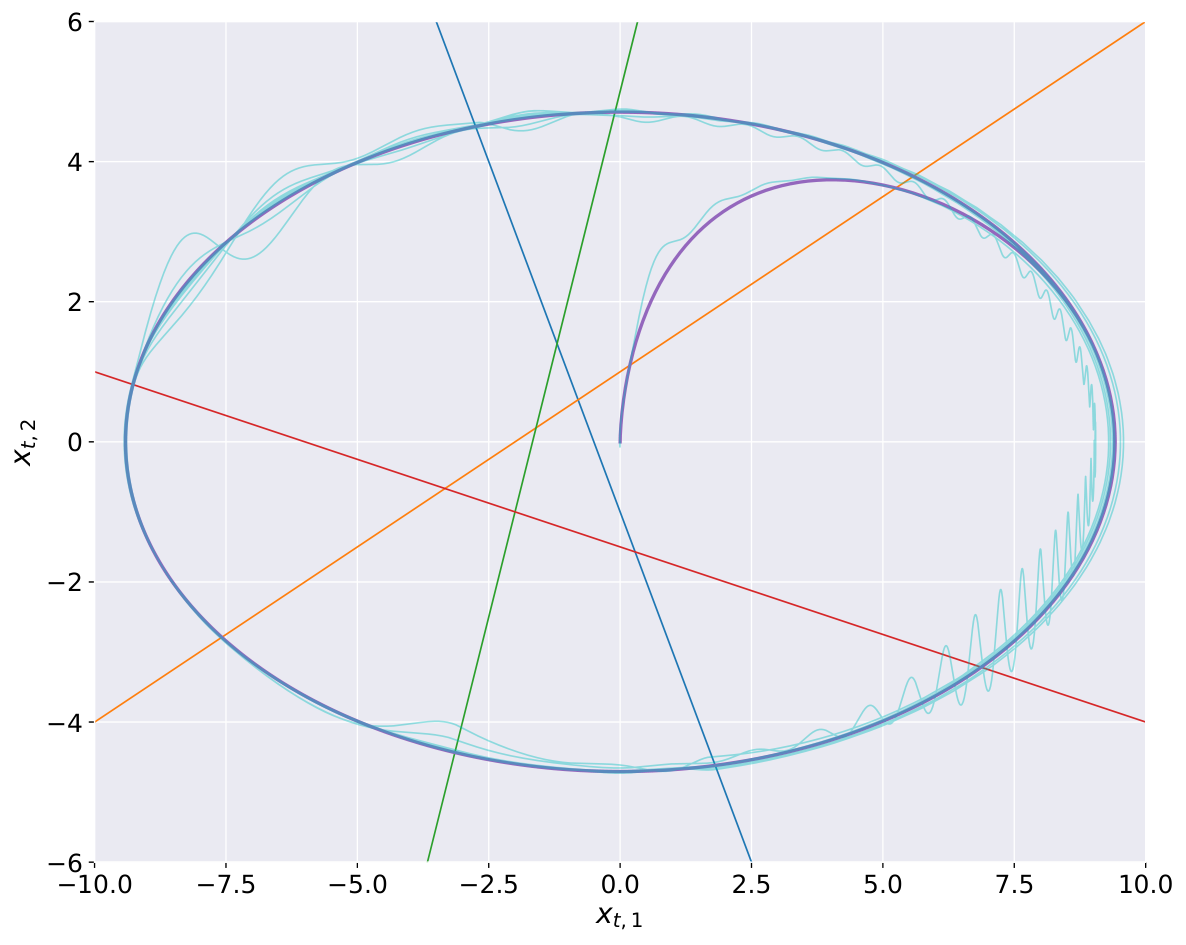
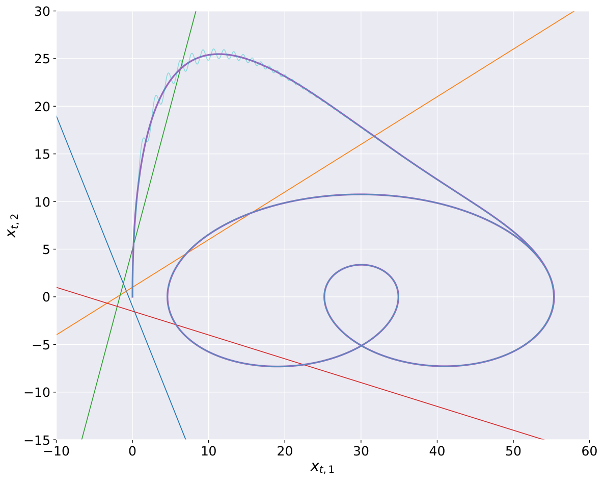
The resulting plant and reference state trajectories $x_{t}$ and $x_{t}^{r}$ are plotted in state space along with the hyperplanes $W^{\top}x+b=0_{4}$, in Figure 2 and Figure 3 respectively for the two scenarios. We see clearly that the limit cycles in both cases stay within a compact set $\mathcal{B}\in\mathbb{R}^{2}$, and so the ReLU activations within $\phi$ are bounded on this $\mathcal{B}$, and the trajectories never maintain a linear path.

In the first case, the state trajectories cross all $N=4$ hyperplanes at nondegenerate borders persistently, as well as never being parallel to any subset of active hyperplanes, thus meeting the criteria of Theorem 2. In the second case, the limit cycle only crosses two of the hyperplanes persistently.

The parameter estimation error $\|{\widehat{\Theta}}_{t}-\Theta\|_{2}$ for both cases is plotted over simulation time in Fig. 4. For the case with $r_{t}^{(1)}$, we see that the error converges to zero as the parameter estimators converge to the true values, while for the case with $r_{t}^{(2)}$ the error does not converge and is well above zero.

References

- [1] Shankar Sastry and Marc Bodson “Adaptive control: stability, convergence and robustness” Prentice Hall, Inc., 1989
- [2] Jean-Jacques Slotine and Weiping Li “Applied nonlinear control” Prentice hall Englewood Cliffs, NJ, 1991
- [3] Eugene Lavretsky and Kevin Wise “Robust and Adaptive Control: with Aerospace Applications” Springer, 2013
- [4] AP Morgan and KS Narendra “On the uniform asymptotic stability of certain linear nonautonomous differential equations” In SIAM Journal on Control and Optimization 15.1 SIAM, 1977, pp. 5–24
- [5] Brian Anderson “Exponential stability of linear equations arising in adaptive identification” In IEEE Transactions on Automatic Control 22.1 IEEE, 1977, pp. 83–88
- [6] Veronica Adetola and Martin Guay “Finite-time parameter estimation in adaptive control of nonlinear systems” In IEEE Transactions on Automatic Control 53.3 IEEE, 2008, pp. 807–811
- [7] Sayan Roy, Shubhendu Bhasin and Indra Kar “Combined MRAC for unknown MIMO LTI systems with parameter convergence” In IEEE Transactions on Automatic Control 63.1 IEEE, 2017, pp. 283–290
- [8] Girish Chowdhary, Tansel Yucelen, Maximillian M“”uhlegg and Eric Johnson “Concurrent learning adaptive control of linear systems with exponentially convergent bounds” In International Journal of Adaptive Control and Signal Processing 27.4 Wiley Online Library, 2013, pp. 280–301
- [9] Anuradha Annaswamy et al. “Online Algorithms and Policies Using Adaptive and Machine Learning Approaches” In arXiv preprint arXiv:2105.06577, 2021
- [10] Jan Willems, Paolo Rapisarda, Ivan Markovsky and Bart De “A note on persistency of excitation” In Systems & Control Letters 54.4 Elsevier, 2005, pp. 325–329
- [11] Kamil Nar and S Sastry “Persistency of excitation for robustness of neural networks” In arXiv preprint arXiv:1911.01043, 2019
- [12] Elena Panteley, Antonio Loria and Andrew Teel “Relaxed persistency of excitation for uniform asymptotic stability” In IEEE Transactions on Automatic Control 46.12 IEEE, 2001, pp. 1874–1886
- [13] Riccardo Marino and Patrizio Tomei “Global adaptive output-feedback control of nonlinear systems. I. Linear parameterization” In IEEE Transactions on Automatic Control 38.1 IEEE, 1993, pp. 17–32
- [14] Hassan Khalil “High-gain observers in nonlinear feedback control” SIAM, 2017
- [15] Stephen Boyd and Sosale Sastry “Necessary and sufficient conditions for parameter convergence in adaptive control” In Automatica 22.6 Elsevier, 1986, pp. 629–639
- [16] Iven Mareels and Michel Gevers “Persistency of excitation criteria for linear, multivariable, time-varying systems” In Mathematics of Control, Signals and Systems 1.3 Springer, 1988, pp. 203–226
- [17] Gerhard Kreisselmeier and Gudrun Rietze-Augst “Richness and excitation on an interval-with application to continuous-time adaptive control” In IEEE transactions on automatic control 35.2 IEEE, 1990, pp. 165–171
- [18] Jung-Shan Lin and Ioannis Kanellakopoulos “Nonlinearities enhance parameter convergence in strict feedback systems” In IEEE Transactions on Automatic Control 44.1 IEEE, 1999, pp. 89–94
- [19] Philipp Karg, Florian K“”opf, Christian Braun and S“”oren Hohmann “Excitation for Adaptive Optimal Control of Nonlinear Systems in Differential Games” In IEEE Transactions on Automatic Control IEEE, 2022
- [20] Alberto Padoan, Giordano Scarciotti and Alessandro Astolfi “A geometric characterization of the persistence of excitation condition for the solutions of autonomous systems” In IEEE Transactions on Automatic Control 62.11 IEEE, 2017, pp. 5666–5677
- [21] Juan Rueda-Escobedo and Jaime Moreno “Strong Lyapunov functions for two classical problems in adaptive control” In Automatica 124 Elsevier, 2021, pp. 109250
- [22] AJ Kurdila, Francis Narcowich and Joseph Ward “Persistency of excitation in identification using radial basis function approximants” In SIAM journal on control and optimization 33.2 SIAM, 1995, pp. 625–642
Appendix A Proofs of Theorems 1 and 2
Here we will prove the main results provided in Section IV.
A-A Proof Methodology and Setup
The proofs for both theorems rely on the same contradiction method and share a common setup.
First, we will assume that the state trajectory is continuous and stays within some
compact set for all , and that the component activations
of are then bounded on that
.
Then we will assume that for any shift of the time window of any
length , there exists a nonzero vector such that