跳到论文正文
W Papers独立论文阅读器 arXiv:2209.06276 论文正文 计算阅读时间 · 0%
引用这篇论文根据当前论文元数据生成,正式投稿前建议核对。


License: CC BY 4.0
arXiv:2209.06276v1 [q-fin.PR] 13 Sep 2022

ESG-Valued Discrete Option Pricing in Complete Markets

Yuan Hu Affiliation: Department of Mathematics, University of California San Diego, La Jolla, CA 92093, U.S.A.
yuh099@ucsd.edu
   W. Brent Lindquist Affiliation: Department of Mathematics & Statistics, Texas Tech University, Lubbock, TX 79409-1042, U.S.A.
zari.rachev@ttu.edu
Affiliation:  Corresponding author, brent.lindquist@ttu.edu
   Svetlozar T. Rachev Affiliation: Department of Mathematics & Statistics, Texas Tech University, Lubbock, TX 79409-1042, U.S.A.
zari.rachev@ttu.edu

Abstract We consider option pricing using replicating binomial trees, with a two fold purpose. The first is to introduce ESG valuation into option pricing. We explore this in a number of scenarios, including enhancement of yield due to trader information and the impact of the past history of a market driver. The second is to emphasize the use of discrete dynamic pricing, rather than continuum models, as the natural model that governs actual market practice. We further emphasize that discrete option pricing models must use discrete compounding (such as risk-free rate compounding of 1+rf​Δ​t1+r_{f}\Delta t) rather than continuous compounding (such as OPENerf​Δ​t)e^{r_{f}\Delta t}).

Keywords ESG scores; dynamic asset pricing; discrete option pricing

1 Introduction

Socially responsible investing (SRI) is an umbrella term for investment in activities and companies that generate positive social and environmental impact. Emerging within the this broad framework (Daugaard, 2020) is a focus on ESG ratings; methodologies under which corporate and investment structures are evaluated under three performance/risk categories: environmental, social, and governance. ESG investing is experiencing fast and inexorable growth; increasing numbers of institutional investors, such as mutual and pension funds, provide socially responsible financial products (Boffo & Patalano, 2020); and increasing numbers of agencies are providing ratings (Amel-Zadeh & Serafeim, 2018). Research highlights two main reasons behind the push towards SRI products: ethical beliefs and improved financial performance (Hartzmark and Sussman, 2019; Bénabou and Tirole, 2010; Krüger, 2015; Lins et al., 2017; Liang and Renneboog, 2017; Starks et al., 2017). How ESG factors are integrated into investment decisions is varied, including: as (positive or negative) screening tools; as a thematic investment; or to tilt a portfolio (Amel-Zadeh & Serafeim, ibid). There is also evidence (Amel-Zadeh & Serafeim, ibid; Berry and Junkus, 2013) that investors focus on different aspects of SRI compared to the developers of socially responsible financial products. There remains a great deal of subjectivity as to how SRI factors, in particular ESG scores, are utilized in the investment universe.

In this article we focus on an empirical pricing model that incorporates ESG scores to produce an ESG-valued return and, consequently, a numeraire that serves as an ESG-valued “price” which reflects a value assignment based upon a combination of financial return and ESG-score. We explore this ESG-valuation model in the context of pricing European contingency claims, specifically call options. Our model introduces an ESG-intensity parameter, λ∈[0,1]\lambda\in[0,1], that designates the relative weight by which a trader values “ESG return” against traditional financial return. In a manner analogous to implied volatility, by comparing model option prices against market data we can extract ESG-intensity surfaces that can be interpreted as reflecting the implicit weighting given to ESG value in formulating option prices as functions of moneyness and time to maturity.

The celebrated Black and Scholes (1973) and Merton (1973) option pricing model (BSM), which is based upon the stochastic differential equation d​St=μ​St​d​t+σ​St​d​BtdS_{t}=\mu S_{t}dt+\sigma S_{t}dB_{t}, where BtB_{t} is a standard Brownian motion, naturally leads to the consideration of a continuous logarithmic return (log-return) process. One consequence of the BSM model is that its option pricing formula only retains the variance of the log-return process, the drift μ\mu in the price process is lost. In addition, the Gaussian nature of the BSM model assumes equal upturn and downturn return probabilities (i.e. p(u)=p(d)=0.5p^{(\text{u})}=p^{(\text{d})}=0.5), disallowing for other possibilities. The classic Cox-Ross-Rubinstein (1970) and Jarrow-Rudd (1983) models, as well as more general discrete pricing models (e.g. Kim et al., 2016, 2019; Hu et al. 2020a, 2020b) have been built to extend the continuum BSM model to capture more of the stylized facts and microstructure of actual market price processes.

One lasting impact of the BSM model has been the motivation to explore the continuum limit of each discrete model, in part to explore which stylized facts or microstructural parameters encapsulated within the discrete model survive into the continuum limit (Kim et al. 2016, 2019; Hu et al. 2020a, 2020b). Obtaining these continuum limits has required the development of binomial trees based upon non-classical invariance principles (Cherny et al., 2003; Davydov and Rotar, 2008). Our motivation to stay within the realm of discrete pricing is two fold. One is based upon the reality that all trading practices take place in discrete time intervals.11 1 Currently bounded below by Δ​t∼10−6\Delta t\sim 10^{-6} seconds, as established by ultra-high frequency traders. However this rate is never realized over a full 24-hour period, but generally over a “working day” of ∼6.5\sim 6.5 hours. The second is that taking the continuum limit of these discrete models leads to loss of some of this microstructure, making continuum limit models less useful.

Log-returns ln⁡(St+d​t/St)\ln(S_{t+dt}/S_{t}) are a critical component of continuum pricing theory, as they make continuum theories analytically tractable. However, every practical use of returns in the market involves discrete (arithmetic) returns (St+Δ​t−St)/St(S_{t+\Delta t}-S_{t})/S_{t} over discrete trading intervals. In this article we explicitly compare binomial pricing trees that naturally invoke either arithmetic (discretely compounded) or logarithmic (continuously compounded) returns. For daily (and intra-day) returns on stocks, the difference between the arithmetic return process and the log-return process is generally small.22 2 However differences compounded over longer time frames may become significant. For option pricing, which is a more complex nonlinear process, our results demonstrate that significant differences can arise between discretely and continuously compounded models (for example, in implied volatility surfaces). In fact, using continuous compounding for the riskless rate when trading of the underlying stock occurs in discrete time increments makes a market composed of a stock, a riskless bond, and an option inconsistent with the fundamental theorem of asset pricing (Delbaen and Schachmayer, 1994; Jarrow et al., 2009). In section 2 we explicitly note how retention of the no-arbitrage condition requires the use of discrete compounding when using discrete pricing models.

This paper is organized as follows. Section 2 introduces the ESG-valued, recombining, binomial tree models designed for arithmetic and log-returns. These ESG-valued models are applied to equity data, and implied surfaces for the ESG-intensity parameter are computed. Section 3 extends the ESG-valued models to markets in which there is an informed trader. Implied surfaces are computed for the trader’s information intensity. These surfaces can be interpreted as indicators of how option traders subjectively weight ESG scores. In section 4 we extend the ESG-valued models of section 2 to the case in which the direction of price change for the underlying stock is influenced by a market driver. Using an extended formulation of the Cherny-Shiryaev-Yor (2003) principle, we introduce history dependence into this asset pricing. Implied surfaces for the ESG-intensity parameter under this formulation are recomputed for the same set of equities and compared with those from section 2. As each model is presented, its continuum limit is presented and the model parameters identified that are contained in the binomial tree model but lost in the continuum limit. Final discussion is presented in section 5.

2 ESG-valued binomial option pricing models

Consider a Black-Scholes-Merton market consisting of a risky asset 𝒮\mathcal{S}, a riskless asset (a bond) ℬ\mathcal{B}, and a European contingent claim (specifically a call option) 𝒞\mathcal{C} having 𝒮\mathcal{S} as the underlying. Over the time interval [0,T][0,T], the dynamics of the prices of 𝒮,ℬ\mathcal{S},\mathcal{B} and 𝒞\mathcal{C} are modeled on a discrete, recombining binomial tree. We allow for variable trading times over this interval by a time-partition parameterized by the integer n∈{1,2,…}n\in\{1,2,\dots\}. For a choice of nn, the partition is tn,k;k=1,…,knt_{n,k};\ k=1,\dots,k_{n}, where 0=tn,0<tn,1⋯<tn,kn=T0=t_{n,0}<t_{n,1}\cdots<t_{n,k_{n}}=T denote the trading times. Let Δ​tn,k=tn,k−tn,k−1\Delta t_{n,k}=t_{n,k}-t_{n,k-1} denote the duration between successive trades.

We introduce ESG-valuation into option pricing by defining the ESG-valued return, whether logarithmic or arithmetic,33 3 Using (1) for both logarithmic and arithmetic returns is justified under the assumption that, for Δ​tn,k+1\Delta t_{n,k+1} sufficiently small, ln⁡(Stn,k,λ/Stn,k−1,λ)≈Stn,k,λ/Stn,k−1,λ−1\ln\left(S_{t_{n,k},\lambda}/S_{t_{n,k-1},\lambda}\right)\approx S_{t_{n,k},\lambda}/S_{t_{n,k-1},\lambda}-1. by

rtn,k,λ=λ​etn,k+(1−λ)​rtn,k,0.r_{t_{n,k},\lambda}=\lambda e_{t_{n,k}}+(1-\lambda)r_{t_{n,k},0}\,. (1)

Here rtn,k,0=rtn,k,λ=0r_{t_{n,k},0}=r_{t_{n,k},\lambda=0} denotes the usual financial return at trading time tn,kt_{n,k} and etn,ke_{t_{n,k}} is a normalized ESG score. We refer to the weight parameter λ∈[0,1]\lambda\in[0,1] as the ESG intensity. As ESG scores, ESGtn,k\text{ESG}_{t_{n,k}}, are provided in a range ESGtn,k∈[ESGmin,ESGmax]\text{ESG}_{t_{n,k}}\in[\text{ESG}_{\text{min}},\text{ESG}_{\text{max}}], where typically ESGmin=0\text{ESG}_{\text{min}}=0 and ESGmax=100\text{ESG}_{\text{max}}=100, etn,ke_{t_{n,k}} is a normalized ESGtn,k\text{ESG}_{t_{n,k}} value scaled to the range [−1/c,1/c][-1/c,1/c]. The constant c∈Rc\in R insures that the ranges of etn,ke_{t_{n,k}} and rtn,k,0r_{t_{n,k},0} are comparable.44 4 For daily return data, where Δ​tn,k=1\Delta t_{n,k}=1 trading day, we use the value c=252c=252, assuming 252 trading days per calendar year. We consider two models for the pricing of options pertinent to an ESG-value trader who holds a short position in the 𝒞\mathcal{C}-contract and trades at the discrete times tn,kt_{n,k}.

ESG-valued arithmetic return model. Based on arithmetic returns, the price model for stock 𝒮\mathcal{S} is given by

Sn,k+1,λ={Sn,k+1,λ(u)=Sn,k,λ​(1+Un,k+1,λ), w.p. ​pn,k+1,λ,Sn,k+1,λ(u)=Sn,k,λ​(1+Dn,k+1,λ), w.p. ​1−pn,k+1,λ.S_{n,k+1,\lambda}=\begin{cases}S^{(\textrm{u})}_{n,k+1,\lambda}=S_{n,k,\lambda}\left(1+U_{n,k+1,\lambda}\right),\text{ w.p. }p_{n,k+1,\lambda}\,,\\ S^{(\textrm{u})}_{n,k+1,\lambda}=S_{n,k,\lambda}\left(1+D_{n,k+1,\lambda}\right),\text{ w.p. }1-p_{n,k+1,\lambda}\,.\end{cases} (2)

In (2), and what follows, we use a condensed time notation. It is to be understood that Sn,k,λ(u)≡Stn,k,λ(u)S^{(\text{u})}_{n,k,\lambda}\equiv S^{(\text{u})}_{t_{n,k},\lambda}. Similarly for Sn,k,λ(d)S^{(\text{d})}_{n,k,\lambda}, Sn,k,λS_{n,k,\lambda}, Un,k,λU_{n,k,\lambda}, Dn,k,λD_{n,k,\lambda}, pn,k,λp_{n,k,\lambda}, rn,k,λr_{n,k,\lambda}, and all other time dependent variables. The probability pn,k+1,λp_{n,k+1,\lambda} governs the direction of the price change over the interval [tn,k,tn,k+1)[t_{n,k},t_{n,k+1}). The probabilities pn,k,λp_{n,k,\lambda} are determined by a triangular array of independent Bernoulli random variables ςn,1,λ,ςn,2,λ,…,ςn,kn,λ\varsigma_{n,1,\lambda},\varsigma_{n,2,\lambda},\ldots,\varsigma_{n,k_{n},\lambda}, n={1,2,…}n=\{1,2,\ldots\} satisfying ℙ⁡(ςn,k,λ=1)=1−ℙ⁡(ςn,k,λ=−1)≡pn,k,λ∈(0,1)\mathbb{P}(\varsigma_{n,k,\lambda}=1)=1-\mathbb{P}(\varsigma_{n,k,\lambda}=-1)\equiv p_{n,k,\lambda}\in(0,1), k=1,…,knk=1,\ldots,k_{n}. The pricing tree (2) is adapted to the discrete filtration

𝔽(n,λ)={ℱ(n,k,λ)=σ⁡(ςn,1,λ,ςn,2,λ,…,ςn,k,λ),k=1,…,kn,ℱ(n,0,λ)={∅,Ω}}.\mathbb{F}^{(n,\lambda)}=\left\{\mathcal{F}^{(n,k,\lambda)}=\sigma(\varsigma_{n,1,\lambda},\varsigma_{n,2,\lambda},\ldots,\varsigma_{n,k,\lambda}),\ k=1,\ldots,k_{n},\ \mathcal{F}^{(n,0,\lambda)}=\{\varnothing,\Omega\}\right\}. (3)

The probability pn,k+1,λp_{n,k+1,\lambda} is ℱ(n,k,λ)\mathcal{F}^{(n,k,\lambda)}-measurable.

The price of the riskless asset ℬ\mathcal{B}, generating the risk-free rate of return rf,n,kr_{f,n,k}, evolves as

βn,k+1=βn,k​(1+rf,n,k​Δ​tn,k+1).\beta_{n,k+1}=\beta_{n,k}(1+r_{f,n,k}\Delta t_{n,k+1})\,. (4)

Let fn,k,λf_{n,k,\lambda} denote the price of 𝒞\mathcal{C}. The single time step, risk-neutral relationship for the price of 𝒞\mathcal{C} is

fn,k,λ\displaystyle f_{n,k,\lambda} =11+rf,n,k​Δ​tn,k+1​[qn,k+1,λ​fn,k+1,λ(u)+(1−qn,k+1,λ)​fn,k+1,λ(d)],\displaystyle=\frac{1}{1+r_{f,n,k}\Delta t_{n,k+1}}\left[q_{n,k+1,\lambda}f_{n,k+1,\lambda}^{\text{(u)}}+(1-q_{n,k+1,\lambda})f_{n,k+1,\lambda}^{\text{(d)}}\right], (5)
qn,k+1,λ\displaystyle q_{n,k+1,\lambda} =rf,n,k​Δ​tn,k+1−Dn,k+1,λUn,k+1,λ−Dn,k+1,λ.\displaystyle=\frac{r_{f,n,k}\Delta t_{n,k+1}-D_{n,k+1,\lambda}}{U_{n,k+1,\lambda}-D_{n,k+1,\lambda}}\,.

The risk neutral probability qn,k+1,λq_{n,k+1,\lambda} is ℱ(n,k,λ)\mathcal{F}^{(n,k,\lambda)}-measurable. The conditional mean and variance of the arithmetic return process rn,k+1,λ≡(Sn,k+1,λ−Sn,k,λ)/Sn,k,λr_{n,k+1,\lambda}\equiv(S_{n,k+1,\lambda}-S_{n,k,\lambda})/S_{n,k,\lambda} are

𝔼⁡[rn,k+1,λ|Sn,k,λ]\displaystyle\mathbb{E}\left[r_{n,k+1,\lambda}|S_{n,k,\lambda}\right] =pn,k+1,λ​Un,k+1,λ+(1−pn,k+1,λ)​Dn,k+1,λ,\displaystyle=p_{n,k+1,\lambda}U_{n,k+1,\lambda}+(1-p_{n,k+1,\lambda})D_{n,k+1,\lambda}\,, (6)
Var​[rn,k+1,λ|Sn,k,λ]\displaystyle\text{Var}\left[r_{n,k+1,\lambda}|S_{n,k,\lambda}\right] =pn,k+1,λ​(1−pn,k+1,λ)​[Un,k+1,λ−Dn,k+1,λ]2.\displaystyle=p_{n,k+1,\lambda}(1-p_{n,k+1,\lambda})\left[U_{n,k+1,\lambda}-D_{n,k+1,\lambda}\right]^{2}.

Defining the instantaneous Sharpe ratio over the time period Δ​tn,k+1\Delta t_{n,k+1} as

Θn,k,λ=𝔼⁡(rn,k+1,λ|Sn,k,λ)−rf,n,k​Δ​tn,k+1Var​(rn,k+1,λ|Sn,k,λ)​Δ​tn,k+1,\Theta_{n,k,\lambda}=\frac{\mathbb{E}\left(r_{n,k+1,\lambda}|S_{n,k,\lambda}\right)-r_{f,n,k}\Delta t_{n,k+1}}{\sqrt{\text{Var}\left(r_{n,k+1,\lambda}|S_{n,k,\lambda}\right)\Delta t_{n,k+1}}}\,, (7)

from (6) we have

Θn,k,λ=pn,k+1,λ−rf,n,k​Δ​tn,k+1−Dn,k+1,λUn,k+1,λ−Dn,k+1,λpn,k+1,λ​(1−pn,k+1,λ)​Δ​tn,k+1,\Theta_{n,k,\lambda}=\frac{p_{n,k+1,\lambda}-\frac{r_{f,n,k}\Delta t_{n,k+1}-D_{n,k+1,\lambda}}{U_{n,k+1,\lambda}-D_{n,k+1,\lambda}}}{\sqrt{p_{n,k+1,\lambda}(1-p_{n,k+1,\lambda})\Delta t_{n,k+1}}}\,, (8)

which leads to the identity

qn,k+1,λ=pn,k+1,λ−Θn,k,λ​pn,k+1,λ​(1−pn,k+1,λ)​Δ​tn,k+1.q_{n,k+1,\lambda}=p_{n,k+1,\lambda}-\Theta_{n,k,\lambda}\sqrt{p_{n,k+1,\lambda}(1-p_{n,k+1,\lambda})\Delta t_{n,k+1}}\,. (9)

Matching the instantaneous mean μn,k,λ(r)\mu_{n,k,\lambda}^{(\text{r})} and variance (σn,k,λ(r))2\left(\sigma_{n,k,\lambda}^{(\text{r})}\right)^{2} of the ESG-valued arithmetic return process

𝔼⁡[rn,k+1,λ|Sn,k,λ]=μn,k,λ(r)​Δ​tn,k+1,Var​[rn,k+1,λ|Sn,k,λ]=(σn,k,λ(r))2​Δ​tn,k+1,\mathbb{E}\left[r_{n,k+1,\lambda}|S_{n,k,\lambda}\right]=\mu_{n,k,\lambda}^{(\text{r})}\Delta t_{n,k+1}\,,\qquad\text{Var}\left[r_{n,k+1,\lambda}|S_{n,k,\lambda}\right]=\left(\sigma_{n,k,\lambda}^{(\text{r})}\right)^{2}\Delta t_{n,k+1}\,, (10)

leads to the specific forms

Un,k+1,λ\displaystyle U_{n,k+1,\lambda} =μn,k,λ(r)​Δ​tn,k+1+σn,k,λ(r)​pn,k+1,λ(u)​Δ​tn,k+1,\displaystyle=\mu_{n,k,\lambda}^{(\text{r})}\ \Delta t_{n,k+1}+\sigma_{n,k,\lambda}^{(\text{r})}\ p^{(\text{u})}_{n,k+1,\lambda}\sqrt{\Delta t_{n,k+1}}\,, (11)
Dn,k+1,λ\displaystyle D_{n,k+1,\lambda} =μn,k,λ(r)​Δ​tn,k+1−σn,k,λ(r)​pn,k+1,λ(d)​Δ​tn,k+1,\displaystyle=\mu_{n,k,\lambda}^{(\text{r})}\ \Delta t_{n,k+1}-\sigma_{n,k,\lambda}^{(\text{r})}\ p^{(\text{d})}_{n,k+1,\lambda}\sqrt{\Delta t_{n,k+1}}\,,
pn,k+1,λ(u)\displaystyle p^{(\text{u})}_{n,k+1,\lambda} =1−pn,k+1,λpn,k+1,λ,p(d)n,k+1,λ=pn,k+1,λ1−pn,k+1,λ.\displaystyle=\sqrt{\cfrac{1-p_{n,k+1,\lambda}}{p_{n,k+1,\lambda}}}\,,\qquad\qquad p^{(\text{d})}_{n,k+1,\lambda}=\sqrt{\cfrac{p_{n,k+1,\lambda}}{1-p_{n,k+1,\lambda}}}\,.

The conditional expected mean and variance of the stock price are

𝔼⁡[Sn,k+1,λ|Sn,k,λ]\displaystyle\mathbb{E}\left[S_{n,k+1,\lambda}|S_{n,k,\lambda}\right] =Sn,k,λ​[pn,k+1,λ​(1+Un,k+1,λ)+(1−pn,k+1,λ)​(1+Dn,k+1,λ)]\displaystyle=S_{n,k,\lambda}\left[p_{n,k+1,\lambda}\left(1+U_{n,k+1,\lambda}\right)+(1-p_{n,k+1,\lambda})\left(1+D_{n,k+1,\lambda}\right)\right] (12)
=Sn,k,λ​[1+μn,k,λ(r)​Δ​tn,k+1],\displaystyle=S_{n,k,\lambda}\left[1+\mu_{n,k,\lambda}^{(\text{r})}\ \Delta t_{n,k+1}\right],
Var​[Sn,k+1,λ|Sn,k,λ]\displaystyle\text{Var}\left[S_{n,k+1,\lambda}|S_{n,k,\lambda}\right] =Sn,k,λ2​pn,k+1,λ​(1−pn,k+1,λ)​[Un,k+1,λ−Dn,k+1,λ]2\displaystyle=S_{n,k,\lambda}^{2}\ p_{n,k+1,\lambda}(1-p_{n,k+1,\lambda})\left[U_{n,k+1,\lambda}-D_{n,k+1,\lambda}\right]^{2}
=Sn,k,λ2​(σn,k,λ(r))2​Δ​tn,k+1,\displaystyle=S_{n,k,\lambda}^{2}\ \left(\sigma_{n,k,\lambda}^{(\text{r})}\right)^{2}\Delta t_{n,k+1}\,,

from which we identify the instantaneous drift coefficient μn,k,λ\mu_{n,k,\lambda} and variance σn,k,λ2\sigma_{n,k,\lambda}^{2} of 𝒮\mathcal{S},

μn,k,λ=μn,k,λ(r),σn,k,λ2=(σn,k,λ(r))2.\mu_{n,k,\lambda}=\mu_{n,k,\lambda}^{(\text{r})},\qquad\qquad\sigma_{n,k,\lambda}^{2}=\left(\sigma_{n,k,\lambda}^{(\text{r})}\right)^{2}\,. (13)

Equations (10) through (12) can be trivially re-expressed in terms of μn,k,λ\mu_{n,k,\lambda} and σn,k,λ\sigma_{n,k,\lambda}. Using (11), (8) becomes

Θn,k,λ=μn,k,λ−rf,n,kσn,k,λ≡θn,k,λ,\Theta_{n,k,\lambda}=\frac{\mu_{n,k,\lambda}-r_{f,n,k}}{\sigma_{n,k,\lambda}}\equiv\theta_{n,k,\lambda}\,, (14)

where θn,k,λ\theta_{n,k,\lambda} denotes the market price of risk.

As in Hu et al. (2020b), a non-standard invariance principle (Davydov and Rotar, 2008) can be used to show that the pricing tree (2), (11) generates a D⁡[0,T]D[0,T] stochastic process which converges weakly in Skorokhod D⁡[0,T]D[0,T] topology to the cumulative return process55 5 As defined in Duffie, 2001, section 6D, p. 106. Rt,λR_{t,\lambda}, t∈[0,T]t\in[0,T] determined by d​Rt,λ=d​St,λ/St,λ=μt,λ​d​t+σt,λ​d​BtdR_{t,\lambda}=dS_{t,\lambda}/S_{t,\lambda}=\mu_{t,\lambda}dt+\sigma_{t,\lambda}dB_{t}, where BtB_{t} is a standard Brownian motion. In the risk-neutral world, the limiting process is the same, with μt,λ\mu_{t,\lambda} replaced by rf,tr_{f,t}. We note that the discrete model is much more informative than the continuous time model as it preserves both μtn,k,λ\mu_{t_{n,k},\lambda} and ptn,k,λp_{t_{n,k},\lambda}. Secondly, the discrete formulation leads to binomial models which include additional market microstructure features (Jacod and Ait-Sahaliz, 2014, section 2.2.2; Jarrow et al., 2009).

ESG-valued log-return model. In the second model, which we refer to as the ESG-valued log-return model, the price of 𝒮\mathcal{S} is given by

Sn,k+1,λ={Sn,k+1,λ(u)=Sn,k,λ​eUn,k+1,λ, w.p. ​pn,k+1,λ,Sn,k+1,λ(d)=Sn,k,λ​eDn,k+1,λ, w.p. ​1−pn,k+1,λ.S_{n,k+1,\lambda}=\begin{cases}S^{(\text{u})}_{n,k+1,\lambda}=S_{n,k,\lambda}e^{U_{n,k+1,\lambda}},\text{ w.p. }p_{n,k+1,\lambda}\,,\\ S^{(\text{d})}_{n,k+1,\lambda}=S_{n,k,\lambda}e^{D_{n,k+1,\lambda}},\text{ w.p. }1-p_{n,k+1,\lambda}\,.\end{cases} (15)

The terms Un,k+1,λU_{n,k+1,\lambda} and Dn,k+1,λD_{n,k+1,\lambda} appearing in (15) will be different from those in (2) and hence the price trajectories Sn,k,λS_{n,k},\lambda will differ between the two models. We do not believe the reader will be confused between the similarity in notation when each model is discussed. The probabilities in (15) are also given by a triangular array of independent Bernoulli random variables, consequently the pricing tree (15) is adapted to the discrete filtration (3).

The price of the riskless asset ℬ\mathcal{B} is now given by

βn,k+1=βn,k​erf,n,k​Δ​tn,k+1,\beta_{n,k+1}=\beta_{n,k}e^{r_{f,n,k}\Delta t_{n,k+1}}\,, (16)

and the risk-neutral relation for the price of 𝒞\mathcal{C} is

fn,k,λ\displaystyle f_{n,k,\lambda} =e−rf,n,k​Δ​tn,k+1​[qn,k+1,λ​fn,k+1,λ(u)+(1−qn,k+1,λ)​fn,k+1,λ(d)],\displaystyle=e^{-r_{f,n,k}\Delta t_{n,k+1}}\left[q_{n,k+1,\lambda}f_{n,k+1,\lambda}^{\text{(u)}}+(1-q_{n,k+1,\lambda})f_{n,k+1,\lambda}^{\text{(d)}}\right], (17)
qn,k+1,λ\displaystyle q_{n,k+1,\lambda} =erf,n,k​Δ​tn,k+1−eDn,k+1,λeUn,k+1,λ−eDn,k+1,λ.\displaystyle=\frac{e^{r_{f,n,k}\Delta t_{n,k+1}}-e^{D_{n,k+1,\lambda}}}{e^{U_{n,k+1,\lambda}}-e^{D_{n,k+1,\lambda}}}\,.

The conditional mean and variance of the log-return rn,k+1,λ=ln⁡(Sn,k+1,λ/Sn,k,λ)r_{n,k+1,\lambda}=\ln(S_{n,k+1,\lambda}/S_{n,k,\lambda}) have exactly the same form as (6) and the instantaneous Sharpe ratio has the form (8). However, in this model the identity (9) does not hold.

Matching the instantaneous mean μn,k,λ(r)\mu_{n,k,\lambda}^{(\text{r})} and variance (σn,k,λ(r))2\left(\sigma_{n,k,\lambda}^{(\text{r})}\right)^{2} of the ESG-valued log-return process

𝔼⁡[rn,k+1,λ|Sn,k,λ]=μn,k,λ(r)​Δ​tn,k+1,Var​[rn,k+1,λ|Sn,k,λ]=(σn,k,λ(r))2​Δ​tn,k+1,\mathbb{E}\left[r_{n,k+1,\lambda}|S_{n,k,\lambda}\right]=\mu_{n,k,\lambda}^{(\text{r})}\Delta t_{n,k+1}\,,\qquad\text{Var}\left[r_{n,k+1,\lambda}|S_{n,k,\lambda}\right]=\left(\sigma_{n,k,\lambda}^{(\text{r})}\right)^{2}\Delta t_{n,k+1}\,, (18)

leads to the specific forms,

Un,k+1,λ\displaystyle U_{n,k+1,\lambda} =μn,k,λ(r)​Δ​tn,k+1+pn,k+1,λ(u)​σn,k,λ(r)​Δ​tn,k+1,\displaystyle=\mu_{n,k,\lambda}^{(\text{r})}\Delta t_{n,k+1}+p^{(\text{u})}_{n,k+1,\lambda}\sigma_{n,k,\lambda}^{(\text{r})}\sqrt{\Delta t_{n,k+1}}\,, (19)
Dn,k+1,λ\displaystyle D_{n,k+1,\lambda} =μn,k,λ(r)​Δ​tn,k+1−pn,k+1,λ(d)​σn,k,λ(r)​Δ​tn,k+1,\displaystyle=\mu_{n,k,\lambda}^{(\text{r})}\Delta t_{n,k+1}-p^{(\text{d})}_{n,k+1,\lambda}\sigma_{n,k,\lambda}^{(\text{r})}\sqrt{\Delta t_{n,k+1}}\,,

where pn,k,λ(u)p^{(\text{u})}_{n,k,\lambda} and pn,k,λ(d)p^{(\text{d})}_{n,k,\lambda} are as in (11). Using (19), the instantaneous Sharpe ratio is

Θn,k,λ=μn,k,λ(r)−rf,n,kσn,k,λ(r).\Theta_{n,k,\lambda}=\frac{\mu_{n,k,\lambda}^{(\text{r})}-r_{f,n,k}}{\sigma_{n,k,\lambda}^{(\text{r})}}\,. (20)

The conditional expected mean and variance of the stock price are

𝔼⁡[Sn,k+1,λ|Sn,k,λ]\displaystyle\mathbb{E}\left[S_{n,k+1,\lambda}|S_{n,k,\lambda}\right] =Sn,k,λ​[pn,k+1,λ​eUn,k+1,λ+(1−pn,k+1,λ)​eDn,k+1,λ],\displaystyle=S_{n,k,\lambda}\left[p_{n,k+1,\lambda}e^{U_{n,k+1,\lambda}}+(1-p_{n,k+1,\lambda})e^{D_{n,k+1,\lambda}}\right], (21)
Var​[Sn,k+1,λ|Sn,k,λ]\displaystyle\text{Var}\left[S_{n,k+1,\lambda}|S_{n,k,\lambda}\right] =Sn,k,λ2​pn,k+1,λ​(1−pn,k+1,λ)​[eUn,k+1,λ−eDn,k+1,λ]2.\displaystyle=S_{n,k,\lambda}^{2}\ p_{n,k+1,\lambda}(1-p_{n,k+1,\lambda})\left[e^{U_{n,k+1,\lambda}}-e^{D_{n,k+1,\lambda}}\right]^{2}.

Equations (17) through (21) are exact for this log-return model. From (19), expanding (21) to terms of O⁡(Δ​tn,k+1)O(\Delta t_{n,k+1}) produces

𝔼⁡[Sn,k+1,λ|Sn,k,λ]\displaystyle\mathbb{E}\left[S_{n,k+1,\lambda}|S_{n,k,\lambda}\right] =Sn,k,λ​[1+(μn,k,λ(r)+σn,k,λ(r)22)​Δ​tn,k+1],\displaystyle=S_{n,k,\lambda}\left[1+\left(\mu_{n,k,\lambda}^{(\text{r})}+\frac{{\sigma_{n,k,\lambda}^{(\text{r})}}^{2}}{2}\right)\Delta t_{n,k+1}\right], (22)
Var​[Sn,k+1,λ|Sn,k,λ]\displaystyle\text{Var}\left[S_{n,k+1,\lambda}|S_{n,k,\lambda}\right] =Sn,k,λ2​σn,k,λ(r)2​Δ​tn,k+1.\displaystyle=S_{n,k,\lambda}^{2}{\sigma_{n,k,\lambda}^{(\text{r})}}^{2}\Delta t_{n,k+1}\,.

Thus, to terms of O⁡(Δ​tn,k+1)O(\Delta t_{n,k+1}), we identify the instantaneous drift coefficient μn,k,λ\mu_{n,k,\lambda} and standard deviation σn,k,λ\sigma_{n,k,\lambda} of 𝒮\mathcal{S} as

μn,k,λ=μn,k,λ(r)+(σn,k,λ(r))22,σn,k,λ=σn,k,λ(r).\mu_{n,k,\lambda}=\mu_{n,k,\lambda}^{(\text{r})}+\frac{\left(\sigma_{n,k,\lambda}^{(\text{r})}\right)^{2}}{2}\ ,\qquad\sigma_{n,k,\lambda}=\sigma_{n,k,\lambda}^{(\text{r})}\,. (23)

In terms of μn,k,λ\mu_{n,k,\lambda} and σn,k,λ\sigma_{n,k,\lambda}, (20) becomes

Θn,k,λ=μn,k,λ−σn,k,λ2/2−rf,n,kσn,k,λ;\Theta_{n,k,\lambda}=\frac{\mu_{n,k,\lambda}-\sigma_{n,k,\lambda}^{2}/2-r_{f,n,k}}{\sigma_{n,k,\lambda}}\,; (24)

the conditional mean and variance of the log-return are

𝔼⁡[rn,k+1,λ|Sn,k,λ]=(μn,k,λ−σn,k,λ22)​Δ​tn,k+1,Var​[rn,k+1,λ|Sn,k,λ]=σn,k,λ2​Δ​tn,k+1;\mathbb{E}\left[r_{n,k+1,\lambda}|S_{n,k,\lambda}\right]=\left(\mu_{n,k,\lambda}-\frac{\sigma_{n,k,\lambda}^{2}}{2}\right)\Delta t_{n,k+1}\,,\qquad\text{Var}\left[r_{n,k+1,\lambda}|S_{n,k,\lambda}\right]=\sigma_{n,k,\lambda}^{2}\Delta t_{n,k+1}\,; (25)

the appropriate forms for Un,k+1,λU_{n,k+1,\lambda} and Dn,k+1,λD_{n,k+1,\lambda} in (19) to generate (25) are

Un,k+1,λ\displaystyle U_{n,k+1,\lambda} =[μn,k,λ−σn,k,λ22​(pn,k+1,λ(u))2]​Δ​tn,k+1+pn,k+1,λ(u)​σn,k,λ​Δ​tn,k+1,\displaystyle=\left[\mu_{n,k,\lambda}-\frac{\sigma_{n,k,\lambda}^{2}}{2}\left(p^{(\text{u})}_{n,k+1,\lambda}\right)^{2}\right]\Delta t_{n,k+1}+p^{(\text{u})}_{n,k+1,\lambda}\sigma_{n,k,\lambda}\sqrt{\Delta t_{n,k+1}}\,, (26)
Dn,k+1,λ\displaystyle D_{n,k+1,\lambda} =[μn,k,λ−σn,k,λ22​(pn,k+1,λ(d))2]​Δ​tn,k+1−pn,k+1,λ(d)​σn,k​Δ​tn,k+1;\displaystyle=\left[\mu_{n,k,\lambda}-\frac{\sigma_{n,k,\lambda}^{2}}{2}\left(p^{(\text{d})}_{n,k+1,\lambda}\right)^{2}\right]\Delta t_{n,k+1}-p^{(\text{d})}_{n,k+1,\lambda}\sigma_{n,k}\sqrt{\Delta t_{n,k+1}}\,;

and the risk-neutral probability can be written

qn,k+1,λ=pn,k+1,λ−θn,k,λ​pn,k+1,λ​(1−pn,k+1,λ)​Δ​tn,k+1,q_{n,k+1,\lambda}=p_{n,k+1,\lambda}-\theta_{n,k,\lambda}\sqrt{p_{n,k+1,\lambda}(1-p_{n,k+1,\lambda})\Delta t_{n,k+1}}\,, (27)

where θn,k,λ\theta_{n,k,\lambda} is the market price of risk given in (14). Equations (23) through (27) are understood to hold through terms of the appropriate order of Δ​tn,k+1\Delta t_{n,k+1}, as indicated in each equation.

In the limit Δ​tn,k↓0\Delta t_{n,k}\downarrow 0, the binomial tree (15), (26) approximates a cadlag process which converges weakly in the Skorokhod space D⁡[0,T]D[0,T] to the geometric Brownian motion with time dependent parameters (Hu et al., 2020b)

St,λ=S0​exp⁡[(μt,λ−σt,λ22)​t+σt,λ​Bt],S_{t,\lambda}=S_{0}\exp\left[\left(\mu_{t,\lambda}-\frac{{\sigma_{t,\lambda}}^{2}}{2}\right)t+\sigma_{t,\lambda}B_{t}\right], (28)

where BtB_{t} is a standard Brownian motion.

For either the ESG-valued arithmetic return or log-return models, ESG-valuation at intensity λ∈(0,1]\lambda\in(0,1] produces in an ESG-enhanced dividend yield 𝔻n,k,λ\mathbb{D}_{n,k,\lambda} (relative to λ=0\lambda=0) given by

𝔻n,k,λ=σn,k,0​(Θn,k,λ−Θn,k,0).\mathbb{D}_{n,k,\lambda}=\sigma_{n,k,0}\left(\Theta_{n,k,\lambda}-\Theta_{n,k,0}\right). (29)

The dividend yield in each case can be computed using the appropriate model values for Θn,k,λ\Theta_{n,k,\lambda}. When λ=0\lambda=0, each ESG-valued model reverts to a binomial tree model based upon standard financial returns.

ESG-valued option pricing. With a final price Sn,kn,λ≡ST,λS_{n,k_{n},\lambda}\equiv S_{T,\lambda} at maturity time TT on each node of the price tree obtained by (forward) iteration using either (2) or (15), the initial price C⁡(ST,λ,K)C(S_{T,\lambda},K) of the call option can be evaluated from the final payoff fT=g⁡(ST,λ,K)f_{T}=g(S_{T,\lambda},K) by iterating (5) or (17) backwards on the tree in the usual manner.

Enforcement of no-arbitrage. As noted in the Introduction, use of continuous compounding when trading can only occur at discrete times violates the fundamental theorem of asset pricing and the condition of no-arbitrage. This can be seen explicitly by contrasting equations (5) and (17) in the two models considered above. For a discrete pricing process, ensuring positive asset prices and no arbitrage over any discrete time period requires the condition (Shreve, 2004, Chapter 1)

0<1+Dn,k+1,λ<1+rf,n,k​Δ​tn,k+1<1+Un,k+1,λ.0<1+D_{n,k+1,\lambda}<1+r_{f,n,k}\Delta t_{n,k+1}<1+U_{n,k+1,\lambda}\,. (30)

This condition guarantees that the value of the risk-neutral probability qn,k+1,λq_{n,k+1,\lambda} in (5) remains bounded in the interval [0,1][0,1]. However (30) does not guarantee that the value of the risk-neutral probability qn,k+1,λq_{n,k+1,\lambda} in (17) remains so bounded. While (5) is exact, the approximation (27) to (17) only holds if terms of 𝒪⁡(Δ​tn,k+1)\mathcal{O}(\Delta t_{n,k+1}) are ignored. As will be shown in the results below, the presence of these 𝒪⁡(Δ​tn,k+1)\mathcal{O}(\Delta t_{n,k+1}) terms can result in significant differences between implied volatility surfaces computed for the two models. Thus, there is a significant risk in using continuum rates (eUn,k+1,λe^{U_{n,k+1,\lambda}}, eDn,k+1,λe^{D_{n,k+1,\lambda}}, erf,n,k​Δ​tn,k+1e^{r_{f,n,k}\Delta t_{n,k+1}}) in discrete pricing models. (Such usage of continuum rates in discrete models is commonly presented; see, e.g., Chapter 12.8 of the text book by Hull (2012).)

2.1 Application to equity data

We apply both ESG-valued pricing models to equity data using ESG scores obtained from RobecoSAM (now S&P Global).66 6 S&P Global RobecoSAM ESG ratings data provided through Bloomberg Professional Services. We consider daily closing price data for the period 12/31/2020 through 12/31/2021 for three equities, MSFT, AMZN and AAPL. These three equities were chosen as they have, respectively, high, intermediate and low ESG scores over this time period. As is currently the case with most data providers, updated RobecoSAM scores are released once per year; for our time period, new RobecoSAM scores ESG(R)\text{ESG}^{(\text{R})} were released on 11/19/2020 and 11/19/2021. The raw scores ESG(R)\text{ESG}^{(\text{R})} are on a scale of 0 to 100. The daily en,ke_{n,k} values required in (1), were therefore computed as follows

en,k=ESG(R)−5050⋅252.e_{n,k}=\frac{\text{ESG}^{(\text{R})}-50}{50\cdot 252}\,. (31)

where ESG(R)\text{ESG}^{(\text{R})} is understood to refer to the most recent value released prior to day tn,kt_{n,k}. The raw ESG(R)\text{ESG}^{(\text{R})} and scaled en,ke_{n,k} ESG values for 11/19/2020 and 11/19/2021 are given in Table 1.

Table 1: ESG values and stock closing prices S0S_{0}
Equity 11/19/2020 11/19/2021 S0S_{0}\ \ \
ESG(R){}^{(\text{R})} en,ke_{n,k}\ \ \ \ ESG(R){}^{(\text{R})} en,ke_{n,k}\ \ \ \ (USD)
MSFT 96 3.65⋅10−3\ \ 3.65\cdot 10^{-3} 98 3.81⋅10−3\ \ 3.81\cdot 10^{-3} 336.32
AMZN 60 0.79⋅10−3\ \ 0.79\cdot 10^{-3} 71 1.67⋅10−3\ \ 1.67\cdot 10^{-3} 3,334.34
AAPL 25 −1.98⋅10−3-1.98\cdot 10^{-3} 34 −1.27⋅10−3-1.27\cdot 10^{-3} 177.57

We first explore the effects of the addition of ESG-valuation to the financial return in (1). Using the daily closing prices for the three stocks, we compute arithmetic returns rn,k,0r_{n,k,0}. For values of λ∈{0.25,0.5,0.75}\lambda\in\{0.25,0.5,0.75\} we compute ESG-valued returns rn,k,λr_{n,k,\lambda} (assumed to be arithmetic returns) from (1) and subsequently ESG-valued ‘‘prices’’.77 7 The ESG-valued returns (1) effectively generate an ESG-numeraire that we will refer to as an ESG-valued price, or more concisely an ESG price. Fig. 1 plots the resultant ESG price time series for the three stocks over the period 12/31/2020 through 12/31/2021 computed using the values λ∈{0,0.25,0.5,0.75}\lambda\in\{0,0.25,0.5,0.75\}. For comparison purposes, the initial ESG price (on 12/30/2020) for each equity is scaled to unit value. Thus the λ=0\lambda=0 time series correspond to published closing prices rescaled to having a unit value on 12/30/2020.

Refer to caption
Figure 1: (left) ESG-valued price dynamics for chosen values of λ\lambda. For comparison purposes, the initial ESG prices (on 12/30/2020) are scaled to unit value. (right) Box-whisker summaries of the values of the arithmetic returns rn,k,λr_{n,k,\lambda}.

Price values for the two highest ESG scored stocks, MSFT and AMZN, increase with λ\lambda; for the lowest ESG rated stock, AAPL, price values decrease as λ\lambda increases. This behavior can be explained by examining the box-whisker summaries of the ESG-valued returns presented in Fig. 1. As λ\lambda increases, the range of return values decreases due to the higher weighting on en,ke_{n,k} which only changes value once for each stock during this time period. As λ\lambda increases, the average value of rn,k,λr_{n,k,\lambda}: increases for MSFT; increases very slightly for AMZN; and decreases for AAPL, becoming negative for λ=0.5\lambda=0.5 and 0.75.

When rn,k,0r_{n,k,0} is computed using log-returns, for a fixed value of λ>0\lambda>0, equation (1) generates slightly smaller ESG log-return values than when rn,k,0r_{n,k,0} is computed using arithmetic returns. Thus the price series computed from (1) using log-returns for rn,k,0r_{n,k,0} (and interpreting the returns in (1) as log-returns) will be very slightly below88 8 The decrease is greatest for MSFT when λ=0.5\lambda=0.5, producing a price lower by approximately 0.00940.0094 units of account (0.47%0.47\%) after one year. those shown in Fig. 1.

We next consider option pricing based upon the models (2) and (15). To compute option prices, the parameters μn,k,λ\mu_{n,k,\lambda}, σn,k,λ\sigma_{n,k,\lambda} and pn,k,λp_{n,k,\lambda} must be estimated from the appropriate return data using either (13) or (23). We consider option prices computed for tn,k=t_{n,k}= 12/31/2021 based upon each of the three stocks as the underlying. For a given value of λ\lambda and each stock, the estimates μn,k,λ≡μ^λ\mu_{n,k,\lambda}\equiv\hat{\mu}_{\lambda} and σn,k,λ≡σ^λ\sigma_{n,k,\lambda}\equiv\hat{\sigma}_{\lambda} were obtained using the equity’s ESG-valued return data over the period 1/1/2021 through 12/31/2021. The probability estimate pn,k+1,λ≡p^λp_{n,k+1,\lambda}\equiv\hat{p}_{\lambda} was computed as the proportion of the number of days with non-negative values of the equity’s ESG-valued return over this period. The parameter estimates are given in Table 2 for values of λ∈{0,0.25,0.5,0.75}\lambda\in\{0,0.25,0.5,0.75\}.

Table 2: Parameter estimates for 12/31/2021 for the ESG-valued models
Equity μ^0\hat{\mu}_{0} μ^0.25\hat{\mu}_{0.25} μ^0.5\hat{\mu}_{0.5} μ^0.75\hat{\mu}_{0.75} σ^0\hat{\sigma}_{0} σ^0.25\hat{\sigma}_{0.25} σ^0.5\hat{\sigma}_{0.5} σ^0.75\hat{\sigma}_{0.75} p^0\hat{p}_{0} p^0.25\hat{p}_{0.25} p^0.5\hat{p}_{0.5} p^0.75\hat{p}_{0.75}
(×10−3)\left(\times 10^{-3}\right) (×10−2)\left(\times 10^{-2}\right)
arithmetic return
MSFT 1.76 2.24 2.72 3.19 1.33 0.99 0.66 0.33 0.52 0.57 0.66 0.85
AMZN 0.21 0.38 0.55 0.72 1.52 1.14 0.76 0.38 0.51 0.52 0.54 0.60
AAPL 1.31 0.50 -0.30 -1.11 1.58 1.19 0.79 0.40 0.52 0.51 0.46 0.36
log-return
MSFT 1.76 2.22 2.69 3.18 1.32 0.99 0.66 0.33 0.52 0.57 0.66 0.85
AMZN 0.21 0.36 0.52 0.70 1.52 1.14 0.76 0.38 0.51 0.52 0.54 0.60
AAPL 1.30 0.48 -0.33 -1.12 1.58 1.19 0.79 0.40 0.52 0.51 0.46 0.36

Over this time period, MSFT had the largest values for μ^λ\hat{\mu}_{\lambda} and p^λ\hat{p}_{\lambda}, and the smallest values of σ^λ\hat{\sigma}_{\lambda}. As the scaled ESG-values for MSFT and AMZN are positive, μ^λ\hat{\mu}_{\lambda} increases with λ\lambda. With positive scaled ESG-values, the λ​en,k\lambda e_{n,k} term in (1) increases the proportion of positive return values rn,k,λr_{n,k,\lambda} compared to that for rn,k,0r_{n,k,0}. Consequently p^λ\hat{p}_{\lambda} increases with λ\lambda, growing more rapidly for the higher ESG-valued stock. As the scaled ESG-values for AAPL are negative, both μ^λ\hat{\mu}_{\lambda} and p^λ\hat{p}_{\lambda} decrease as λ\lambda increases. For all three equities, as ESG values change only once, on 11/19/2021, σ^λ\hat{\sigma}_{\lambda} decreases as λ\lambda increases.

Implied ESG intensity surfaces. Using the stock prices (shown in Table 1) and the ESG and parameter value estimates for 12/31/2021, for a given maturity time TT and strike price KK the implied ESG intensity λ(i)​(T,K)\lambda^{(i)}(T,K) for stock ii was estimated using the relative mean-square minimization

λ(i)​(T,K)=arg​minλ⁡(C(i)​(ST,K,rf,μ^λ,σ^λ,p^λ)−C(i)​(ST,K)C(i)​(ST,K))2.\lambda^{(i)}(T,K)=\argmin_{\lambda}\left(\frac{C^{(i)}(S_{T},K;r_{f},\hat{\mu}_{\lambda},\hat{\sigma}_{\lambda},\hat{p}_{\lambda})-C^{(i)}(S_{T},K)}{C^{(i)}(S_{T},K)}\right)^{2}. (32)

Here C(i)​(ST,K,r,μ^λ,σ^λ,p^λ)C^{(i)}(S_{T},K;r,\hat{\mu}_{\lambda},\hat{\sigma}_{\lambda},\hat{p}_{\lambda}) represents call option prices based upon the appropriate binomial tree and C(i)​(ST,K)C^{(i)}(S_{T},K) are market call option prices for stock ii obtained from Cboe price quotes for 12/31/2021.99 9 On this date, call option prices for these assets had the maturity dates ranging from 01/21/2022 to 07/15/2022. The data set consisted of 699 AAPL, 581 MSFT, and 1,213 AMZN valid call option contracts. In computing values for C(i)​(ST,K,r,μ^λ,σ^λ,p^λ)C^{(i)}(S_{T},K;r,\hat{\mu}_{\lambda},\hat{\sigma}_{\lambda},\hat{p}_{\lambda}), we used the 10-year U.S. Treasury yield curve rate for 12/31/2021 as the risk-free rate rfr_{f}.1010 10 https://www.treasury.gov. The yearly rate for rfr_{f} on 12/31/2021 was 1.52%1.52\%. As the call option price data is based upon daily changes, we employed an equally spaced partition over the period [0,T=252][0,T=252] giving tn,k=k​Δ​tt_{n,k}=k\Delta t, k=1,…,252k=1,\dots,252 with Δ​t=1\Delta t=1. The minimization (32) was performed over the set of intensities λ∈{0,0.01,0.02,…,1}\lambda\in\{0,0.01,0.02,\ldots,1\} for all K,TK,T values for which the Cboe call option listed a non-zero price.
Refer to caption
Refer to caption
Refer to caption
Refer to caption
Refer to caption
Refer to caption
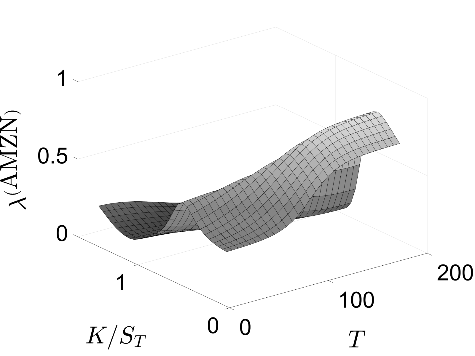
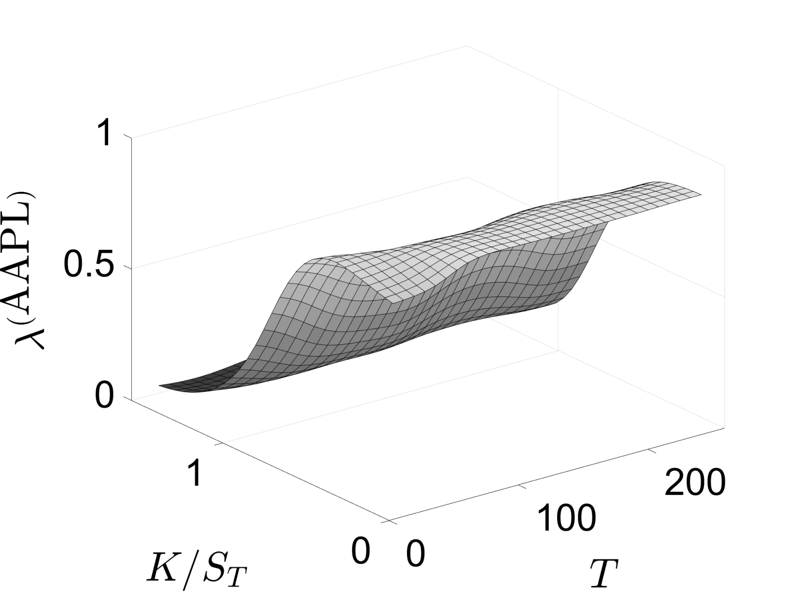
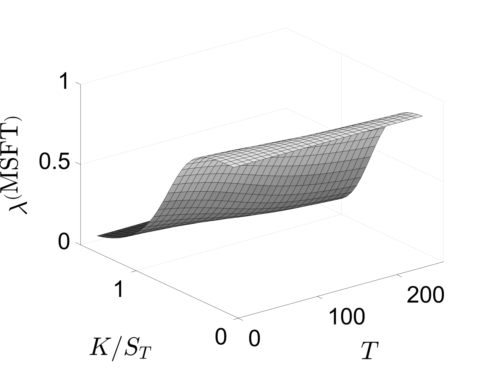
Figure 2: The implied ESG intensity surfaces λ⁡(T,M)\lambda(T,M), plotted as a function of time to maturity TT (in days) and moneyness M=K/STM=K/S_{T}, for the three stocks considered. (top row) Arithmetic return model (2); (bottom) log-return model (15).

Fig. 2 plots the implied ESG intensity surfaces λ⁡(T,M=K/ST)\lambda(T,M=K/S_{T}) as functions of moneyness M=K/STM=K/S_{T} and time to maturity TT computed from the ESG-valued, arithmetic return and log-return models, (2) and (15), respectively. The surfaces are qualitatively similar for all three stocks under the log-return model; greater differences are revealed under the arithmetic model. The value of λ⁡(T,M)\lambda(T,M) is small (ESG ratings are a minor consideration) when options are out-of-the-money and increases (ESG ratings become a greater consideration) as MM moves into-the-money. Generally the dependence of λ\lambda on time to maturity TT is that of a slight increase with TT. The strongest difference is displayed for AMZN under the arithmetic return model, which displays a stronger dependence on TT for in-the-money values of MM.

Implied volatility surfaces. To evaluate the dependence of implied volatility on ESG intensity λ\lambda, we computed the implied volatility σ(i)​(T,M,λ)\sigma^{(i)}(T,M,\lambda) for the values λ∈{0,0.25,0.5,0.75}\lambda\in\{0,0.25,0.5,0.75\} and the same values of TT and KK as for the computations of the implied λ\lambda surfaces. The implied volatility for stock ii was determined by minimizing the relative mean-square difference

σ(i)​(T,K,λ)=arg​minσ⁡(C(i)​(ST,K,rf,μ^λ,p^λ)−C(i)​(ST,K)C(i)​(ST,K))2.\displaystyle\sigma^{(i)}(T,K,\lambda)=\argmin_{\sigma}\left(\frac{C^{(i)}(S_{T},K;r_{f},\hat{\mu}_{\lambda},\hat{p}_{\lambda})-C^{(i)}(S_{T},K)}{C^{(i)}(S_{T},K)}\right)^{2}. (33)

The implied volatilities computed from the arithmetic return model (2) for the three stocks are plotted in Fig. A1 in Appendix A. The implied volatility surface for AMZN shows a characteristic “smile” profile along the moneyness axis, progressing to more of a “smirk” profile as the time-to-maturity increases. In contrast, the implied volatility for MSFT and AAPL display strong “smirk” profiles that remain relatively constant as TT increases. For each stock, the volatility surfaces show comparatively small changes as the ESG intensity λ\lambda increases. This is quantified in Fig. A2, which plots the percent relative changes

Δσ(i)(T,K,λ)=100(σ(i)​(T,K,λ)−σ(i)​(T,K,0)σ(i)​(T,K,0)),λ=0.25,0.5,0.75.\Delta\sigma^{(i)}(T,K,\lambda)=100\left(\frac{\sigma^{(i)}(T,K,\lambda)-\sigma^{(i)}(T,K,0)}{\sigma^{(i)}(T,K,0)}\right),\quad\lambda=0.25,0.5,0.75. (34)

For AAPL and AMZN, and for MSFT when λ≤0.5\lambda\leq 0.5, the percent changes are no more than ±5\pm 5 percent. When λ=0.75\lambda=0.75, relative changes for MSFT approach ±15\pm 15 percent.

Fig. A3 displays the implied volatility surfaces computed from the log-return model (15) for these three stocks. When λ=0\lambda=0, the log-return model surfaces are fairly similar to those for the arithmetic return model in Fig. A1. (The viewing angle is slightly different between Figs. A1 and A3.) As λ\lambda increases, the volatility surface for AMZN remains relatively unchanged. In contrast to the arithmetic return model, much greater changes in implied volatility under the log-return model are observed for MSFT and AAPL as λ\lambda increases. These relative changes for implied volatilities computed for the log-return model are documented in Fig. A4. For MSFT and AMZN, any change in implied volatility is toward smaller values as λ\lambda increases, while for AAPL, any change is toward large values. Very strong changes with λ\lambda are seen far into-the-money at shorter maturity times, with changes approaching −40%-40\% to −60%-60\% for AMZN and MSFT, while changes approach 200%200\% for AAPL.

We also compared the implied volatilities σ(i)​(T,K,λ=0)\sigma^{(i)}(T,K,\lambda=0) computed from (33) against the implied volatility computed using the BSM call option formula C(i,BSM)​(ST,K,rf)C^{(i,\text{BSM})}(S_{T},K;r_{f}),

σ(i,BSM)​(T,K)=arg​minσ⁡(C(i,BSM)​(ST,K,rf)−C(i)​(ST,K)C(i)​(ST,K))2.\displaystyle\sigma^{(i,\text{BSM})}(T,K)=\argmin_{\sigma}\left(\frac{C^{(i,\text{BSM})}(S_{T},K;r_{f})-C^{(i)}(S_{T},K)}{C^{(i)}(S_{T},K)}\right)^{2}. (35)

Fig. A5 shows the BSM implied volatility surfaces σ(i,BSM)\sigma^{(i,\text{BSM})}. In contrast to the discrete models, the implied volatility under BSM shows a “smile” profile for all three stocks (though the range of implied volatility values is small for MSFT under the BSM model). Also plotted in Fig. A5 are the percent relative differences surfaces

Δ​σ(i,BSM)​(T,K,0)=100​(σ(i)​(T,K,0)−σ(i,BSM)​(T,K))/σ(i,BSM)​(T,K),\Delta\sigma^{(i,\text{BSM})}(T,K,0)=100\left(\sigma^{(i)}(T,K,0)-\sigma^{(i,\text{BSM})}(T,K)\right)/\sigma^{(i,\text{BSM})}(T,K)\,, (36)

computed for both the arithmetic or log-return models. Strong differences between each discrete model and the BSM model emerge as values for M=K/STM=K/S_{T} move further into-the-money. The discrete model derives larger volatility values for in-the-money options than does the Black-Scholes-Merton model. The differences are relatively insensitive to change in maturity date.

3 ESG-valued option pricing in markets with informed traders

Following the framework developed in Hu et al. (2020b; section 6), we extend the ESG-valued option pricing model to markets in which there are informed traders. Suppose the ESG-value trader ℵ\aleph has taken a short position in the option contract. The risk neutral portfolio used by ℵ\aleph in section 2 is adjusted to perfectly hedge the short position. We assume a representative investor has complete information on past values of ESG, λ\lambda and returns rn,k,0r_{n,k,0} governing the underlying asset. Assume ℵ\aleph acquires additional information concerning the direction of movement ςn,k,λ\varsigma_{n,k,\lambda} of the underlying. To capitalize on this additional information, ℵ\aleph enters into Nn,k,λ(ℵ)N^{(\aleph)}_{n,k,\lambda} long (or short) forward contracts if the information leads ℵ\aleph to believe the stock price will increase (or decrease). Let pn,k,λ(ℵ)p^{(\aleph)}_{n,k,\lambda} denote the probability that ℵ\aleph’s information is correct. We assume pn,k,λ(ℵ)∈(0.5,1)p^{(\aleph)}_{n,k,\lambda}\in(0.5,1) and utilize the model

pn,k+1,λ(ℵ)=(1+δn,k,λ(ℵ)​Δ​tn,k+1)/2,p^{(\aleph)}_{n,k+1,\lambda}=\left(1+\delta^{(\aleph)}_{n,k,\lambda}\sqrt{\Delta t_{n,k+1}}\right)/2\,, (37)

where 0<δn,k,λ(ℵ)<(Δtn,k+1)−1/20<\delta^{(\aleph)}_{n,k,\lambda}<(\Delta t_{n,k+1})^{-1/2} is ℵ\aleph’s information intensity.

ℵ\aleph’s trading strategy (a combination of trading the stock and forward contracts on the stock) results in the following modification of either option pricing tree (2) or (15).

ESG-valued, arithmetic return, informed model. Conditionally on Sn,k,λS_{n,k,\lambda},

Sn,k+1,λ(ℵ)={Sn,k+1,λ(u)+Nn,k,λ(ℵ)​[Sn,k+1,λ(u)−Sn,k,λ​(1+rf,n,k​Δ​tn,k+1)],w.p.​pn,k+1,λ​pn,k+1,λ(ℵ),Sn,k+1,λ(d)−Nn,k,λ(ℵ)​[Sn,k+1,λ(d)−Sn,k,λ​(1+rf,n,k​Δ​tn,k+1)],w.p.​(1−pn,k+1,λ)​pn,k+1,λ(ℵ),Sn,k+1,λ(u)−Nn,k,λ(ℵ)​[Sn,k+1,λ(u)−Sn,k,λ​(1+rf,n,k​Δ​tn,k+1)],w.p.​pn,k+1,λ​(1−pn,k+1,λ(ℵ)),Sn,k+1,λ(d)+Nn,k,λ(ℵ)​[Sn,k+1,λ(d)−Sn,k,λ​(1+rf,n,k​Δ​tn,k+1)],w.p.​(1−pn,k+1,λ)​(1−pn,k+1,λ(ℵ)),S_{n,k+1,\lambda}^{(\aleph)}=\begin{cases}S_{n,k+1,\lambda}^{(\text{u})}+N^{(\aleph)}_{n,k,\lambda}\left[S_{n,k+1,\lambda}^{(\text{u})}-S_{n,k,\lambda}(1+r_{f,n,k}\Delta t_{n,k+1})\right],\;\textrm{w.p.}\;p_{n,k+1,\lambda}\;p^{(\aleph)}_{n,k+1,\lambda}\,,\\ S_{n,k+1,\lambda}^{(\text{d})}-N^{(\aleph)}_{n,k,\lambda}\left[S_{n,k+1,\lambda}^{(\text{d})}-S_{n,k,\lambda}(1+r_{f,n,k}\Delta t_{n,k+1})\right],\;\textrm{w.p.}\;(1-p_{n,k+1,\lambda})\;p^{(\aleph)}_{n,k+1,\lambda}\,,\\ S_{n,k+1,\lambda}^{(\text{u})}-N^{(\aleph)}_{n,k,\lambda}\left[S_{n,k+1,\lambda}^{(\text{u})}-S_{n,k,\lambda}(1+r_{f,n,k}\Delta t_{n,k+1})\right],\;\textrm{w.p.}\;p_{n,k+1,\lambda}\;\left(1-p^{(\aleph)}_{n,k+1,\lambda}\right),\\ S_{n,k+1,\lambda}^{(\text{d})}+N^{(\aleph)}_{n,k,\lambda}\left[S_{n,k+1,\lambda}^{(\text{d})}-S_{n,k,\lambda}(1+r_{f,n,k}\Delta t_{n,k+1})\right],\;\textrm{w.p.}\;(1-p_{n,k+1,\lambda})\;\left(1-p^{(\aleph)}_{n,k+1,\lambda}\right),\end{cases} (38)

with Sn,0,λ(ℵ)=S0S_{n,0,\lambda}^{(\aleph)}=S_{0}. The terms Sn,k+1,λ(u)S_{n,k+1,\lambda}^{(\text{u})}, and Sn,k+1,λ(d)S_{n,k+1,\lambda}^{(\text{d})}, k=0,1,…,n−1k=0,1,...,n-1, are defined in (2) and (11). To O⁡(Δ​tn,k+1)O(\Delta t_{n,k+1}), the conditional mean and variance of the return rn,k+1,λ(ℵ)r^{(\aleph)}_{n,k+1,\lambda} on ℵ\aleph’s strategy are

𝔼⁡[rn,k+1,λ(ℵ)|Sn,k,λ(ℵ)]\displaystyle\mathbb{E}\left[r_{n,k+1,\lambda}^{(\aleph)}|S_{n,k,\lambda}^{(\aleph)}\right] =(μn,k,λ+σn,k,λ​Nδ(ℵ)​Nn,k,λ(ℵ))​Δ​tn,k+1,\displaystyle=\left(\mu_{n,k,\lambda}+\sigma_{n,k,\lambda}N^{(\aleph)}_{\delta}N^{(\aleph)}_{n,k,\lambda}\right)\Delta t_{n,k+1}\,, (39)
Var​[rn,k+1,λ(ℵCLOSE|Sn,k,λ(ℵ)]\displaystyle\textrm{Var}\left[r_{n,k+1,\lambda}^{(\aleph}|S_{n,k,\lambda}^{(\aleph)}\right] =σn,k,λ2​(1+Nn,k,λ(ℵ)2)​Δ​tn,k+1,\displaystyle={\sigma_{n,k,\lambda}}^{2}\left(1+{N^{(\aleph)}_{n,k,\lambda}}^{2}\right)\Delta t_{n,k+1}\,,

where

Nδ(ℵ)=2​δn,k,λ(ℵ)​pn,k+1,λ​(1−pn,k+1,λ).N^{(\aleph)}_{\delta}=2\delta^{(\aleph)}_{n,k,\lambda}\sqrt{p_{n,k+1,\lambda}(1-p_{n,k+1,\lambda})}\,. (40)

A value for Nn,k,λ(ℵ)N^{(\aleph)}_{n,k,\lambda} can be determined by maximizing ℵ\aleph’s instantaneous Sharpe ratio,

Θn,k,λ(ℵ)=𝔼⁡[rn,k+1,λ(ℵ)|Sn,k,λ(ℵ)]−rf,n,k​Δ​tn,k+1Var​[rn,k,λ(ℵ)|Sn,k,λ(ℵ)]​Δ​tn,k+1=θn,k,λ+Nδ(ℵ)​Nn,k,λ(ℵ)1+Nn,k,λ(ℵ)2,\Theta_{n,k,\lambda}^{(\aleph)}=\frac{\mathbb{E}\left[r_{n,k+1,\lambda}^{(\aleph)}|S_{n,k,\lambda}^{(\aleph)}\right]-r_{f,n,k}\Delta t_{n,k+1}}{\sqrt{\text{Var}\left[r_{n,k,\lambda}^{(\aleph)}|S_{n,k,\lambda}^{(\aleph)}\right]\Delta t_{n,k+1}}}=\frac{\theta_{n,k,\lambda}+N^{(\aleph)}_{\delta}N^{(\aleph)}_{n,k,\lambda}}{\sqrt{1+{N^{(\aleph)}_{n,k,\lambda}}^{2}}}\,, (41)

where θn,k,λ\theta_{n,k,\lambda} is defined in (14). The maximizing value is

Nn,k,λ(ℵ,max)=Nδ(ℵ)θn,k,λ,N^{(\aleph,\text{max})}_{n,k,\lambda}=\frac{N^{(\aleph)}_{\delta}}{\theta_{n,k,\lambda}}\,, (42)

giving the expression for the optimal instantaneous Sharpe ratio,

Θn,k,λ(ℵ,opt)=θn,k,λ2+(Nδ(ℵ))2.\Theta_{n,k,\lambda}^{(\aleph,\text{opt})}=\sqrt{{\theta_{n,k,\lambda}}^{2}+\left(N^{(\aleph)}_{\delta}\right)^{2}}\,. (43)

The optimized conditional mean and variance of the return on ℵ\aleph’s strategy are

𝔼​[rn,k+1,λ(ℵ)|Sn,k,λ(ℵ)](opt)\displaystyle\mathbb{E}\left[r_{n,k+1,\lambda}^{(\aleph)}|S_{n,k,\lambda}^{(\aleph)}\right]^{\text{(opt)}} =[μn,k,λ+σn,k,λ​(Nδ(ℵ))2θn,k,λ]​Δ​tn,k+1,\displaystyle=\left[\mu_{n,k,\lambda}+\frac{\sigma_{n,k,\lambda}\left(N^{(\aleph)}_{\delta}\right)^{2}}{\theta_{n,k,\lambda}}\right]\Delta t_{n,k+1}\,, (44)
Var​[rn,k,λ(ℵCLOSE|Sn,k,λ(ℵ)](opt)\displaystyle\text{Var}\left[r_{n,k,\lambda}^{(\aleph}|S_{n,k,\lambda}^{(\aleph)}\right]^{\text{(opt)}} =σn,k,λ2​[1+(Nδ(ℵ)θn,k,λ)2]​Δ​tn,k+1.\displaystyle={\sigma_{n,k,\lambda}}^{2}\left[1+\left(\frac{N^{(\aleph)}_{\delta}}{\theta_{n,k,\lambda}}\right)^{2}\right]\Delta t_{n,k+1}\,.

ℵ\aleph’s information-enhanced dividend yield 𝔻n,k,λ(ℵ)\mathbb{D}^{(\aleph)}_{n,k,\lambda} is

𝔻n,k,λ(ℵ)=σn,k,λ​(Θn,k,λ(ℵ,opt)−θn,k,λ)=σn,k,λ​[θn,k,λ2+Nδ(ℵ)2−θn,k,λ].\mathbb{D}^{(\aleph)}_{n,k,\lambda}=\sigma_{n,k,\lambda}\left(\Theta_{n,k,\lambda}^{(\aleph,\text{opt})}-\theta_{n,k,\lambda}\right)=\sigma_{n,k,\lambda}\left[\sqrt{{\theta_{n,k,\lambda}}^{2}+{N^{(\aleph)}_{\delta}}^{2}}-\theta_{n,k,\lambda}\right]. (45)

Based on (44), ℵ\aleph’s strategy (38) can be replicated (to O⁡(Δ​tn,k+1)O(\Delta t_{n,k+1})) by the binomial option pricing tree

Sn,k+1,λ(ℵ)={Sn,k,λ(ℵ)​[1+Un,k+1,λ(ℵ)], w.p. ​pn,k+1,λ,Sn,k,λ(ℵ)​[1+Dn,k+1,λ(ℵ)], w.p. ​1−pn,k+1,λ,S^{(\aleph)}_{n,k+1,\lambda}=\begin{cases}S^{(\aleph)}_{n,k,\lambda}\left[1+U^{(\aleph)}_{n,k+1,\lambda}\right],\quad\text{ w.p. }p_{n,k+1,\lambda}\,,\\ S^{(\aleph)}_{n,k,\lambda}\left[1+D^{(\aleph)}_{n,k+1,\lambda}\right],\quad\text{ w.p. }1-p_{n,k+1,\lambda}\,,\end{cases} (46)

where

Un,k+1,λ(ℵ)\displaystyle U^{(\aleph)}_{n,k+1,\lambda} =[μn,k,λ+σn,k,λ​(Nδ(ℵ))2θn,k,λ]​Δ​tn,k+1+pn,k+1,λ(u)​σn,k,λ​[1+(Nδ(ℵ)θn,k,λ)2]​Δ​tn,k+1,\displaystyle=\left[\mu_{n,k,\lambda}+\frac{\sigma_{n,k,\lambda}\left(N^{(\aleph)}_{\delta}\right)^{2}}{\theta_{n,k,\lambda}}\right]\Delta t_{n,k+1}+p_{n,k+1,\lambda}^{(\text{u})}\ \sigma_{n,k,\lambda}\sqrt{\left[1+\left(\frac{N^{(\aleph)}_{\delta}}{\theta_{n,k,\lambda}}\right)^{2}\right]\Delta t_{n,k+1}}\,, (47)
Dn,k+1,λ(ℵ)\displaystyle D^{(\aleph)}_{n,k+1,\lambda} =[μn,k,λ+σn,k,λ​(Nδ(ℵ))2θn,k,λ]​Δ​tn,k+1−pn,k+1,λ(d)​σn,k,λ​[1+(Nδ(ℵ)θn,k,λ)2]​Δ​tn,k+1,\displaystyle=\left[\mu_{n,k,\lambda}+\frac{\sigma_{n,k,\lambda}\left(N^{(\aleph)}_{\delta}\right)^{2}}{\theta_{n,k,\lambda}}\right]\Delta t_{n,k+1}-p_{n,k+1,\lambda}^{(\text{d})}\ \sigma_{n,k,\lambda}\sqrt{\left[1+\left(\frac{N^{(\aleph)}_{\delta}}{\theta_{n,k,\lambda}}\right)^{2}\right]\Delta t_{n,k+1}}\,,

with pn,k+1,λ(u)p_{n,k+1,\lambda}^{(\text{u})} and pn,k+1,λ(d)p_{n,k+1,\lambda}^{(\text{d})} as defined in (11).

ESG-valued, log-return, informed model. Conditionally on Sn,k,λS_{n,k,\lambda},

Sn,k+1,λ(ℵ)={Sn,k+1,λ(u)+Nn,k,λ(ℵ)​[Sn,k+1,λ(u)−Sn,k,λ​exp⁡(rf,n,k​Δ​tn,k+1)],w.p.​pn,k+1,λ​pn,k+1,λ(ℵ),Sn,k+1,λ(d)−Nn,k,λ(ℵ)​[Sn,k+1,λ(d)−Sn,k,λ​exp⁡(rf,n,k​Δ​tn,k+1)],w.p.​(1−pn,k+1,λ)​pn,k+1,λ(ℵ),Sn,k+1,λ(u)−Nn,k,λ(ℵ)​[Sn,k+1,λ(u)−Sn,k,λ​exp⁡(rf,n,k​Δ​tn,k+1)],w.p.​pn,k+1,λ​(1−pn,k+1,λ(ℵ)),Sn,k+1,λ(d)+Nn,k,λ(ℵ)​[Sn,k+1,λ(d)−Sn,k,λ​exp⁡(rf,n,k​Δ​tn,k+1)],w.p.​(1−pn,k+1,λ)​(1−pn,k+1,λ(ℵ)),S_{n,k+1,\lambda}^{(\aleph)}=\begin{cases}S_{n,k+1,\lambda}^{(\text{u})}+N^{(\aleph)}_{n,k,\lambda}\left[S_{n,k+1,\lambda}^{(\text{u})}-S_{n,k,\lambda}\exp(r_{f,n,k}\Delta t_{n,k+1})\right],\;\textrm{w.p.}\;p_{n,k+1,\lambda}\;p^{(\aleph)}_{n,k+1,\lambda}\,,\\ S_{n,k+1,\lambda}^{(\text{d})}-N^{(\aleph)}_{n,k,\lambda}\left[S_{n,k+1,\lambda}^{(\text{d})}-S_{n,k,\lambda}\exp(r_{f,n,k}\Delta t_{n,k+1})\right],\;\textrm{w.p.}\;(1-p_{n,k+1,\lambda})\;p^{(\aleph)}_{n,k+1,\lambda}\,,\\ S_{n,k+1,\lambda}^{(\text{u})}-N^{(\aleph)}_{n,k,\lambda}\left[S_{n,k+1,\lambda}^{(\text{u})}-S_{n,k,\lambda}\exp(r_{f,n,k}\Delta t_{n,k+1})\right],\;\textrm{w.p.}\;p_{n,k+1,\lambda}\;\left(1-p^{(\aleph)}_{n,k+1,\lambda}\right),\\ S_{n,k+1,\lambda}^{(\text{d})}+N^{(\aleph)}_{n,k,\lambda}\left[S_{n,k+1,\lambda}^{(\text{d})}-S_{n,k,\lambda}\exp(r_{f,n,k}\Delta t_{n,k+1})\right],\;\textrm{w.p.}\;(1-p_{n,k+1,\lambda})\;\left(1-p^{(\aleph)}_{n,k+1,\lambda}\right),\end{cases} (48)

with Sn,0,λ(ℵ)=S0S_{n,0,\lambda}^{(\aleph)}=S_{0}. The terms Sn,k+1,λ(u)S_{n,k+1,\lambda}^{(\text{u})}, and Sn,k+1,λ(d)S_{n,k+1,\lambda}^{(\text{d})}, k=0,1,…,n−1k=0,1,...,n-1, are defined in (15) and (26). To O⁡(Δ​t)O(\Delta t) the conditional mean and variance of the return rn,k+1,λ(ℵ)r^{(\aleph)}_{n,k+1,\lambda} on ℵ\aleph’s strategy are1111 11 See Hu et al. (2020b). Care must be taken in the Taylor series expansions of the terms in (48), which have the form ln⁡{(1±N)​exp⁡(U)∓exp⁡rf​Δ​t}\ln\{(1\pm N)\exp(U)\mp\exp{r_{f}\Delta t}\}, to ensure all terms of O⁡(Δ​t)O(\Delta t) and O⁡(Δ​t)O(\sqrt{\Delta t}) are retained. Unfortunately, in Hu et al. (2020b), terms of O⁡((N​Δ​t)2)O((N\sqrt{\Delta t})^{2}) were missed in the computations for the conditional mean.

𝔼⁡(rn,k+1,λ(ℵ)|Sn,k,λ(ℵ))\displaystyle\mathbb{E}\left(r_{n,k+1,\lambda}^{(\aleph)}|S_{n,k,\lambda}^{(\aleph)}\right) =[μn,k,λ−σn,k,λ22​(1+Nn,k,λ(ℵ)2−2​N𝔼(ℵ,δ)​Nn,k,λ(ℵ))]​Δ​tn,k+1,\displaystyle=\left[\mu_{n,k,\lambda}-\frac{{\sigma_{n,k,\lambda}}^{2}}{2}\left(1+{N^{(\aleph)}_{n,k,\lambda}}^{2}-2N^{(\aleph,\delta)}_{\mathbb{E}}N^{(\aleph)}_{n,k,\lambda}\right)\right]\Delta t_{n,k+1}\,,
Var​(rn,k+1,λ(ℵ)|Sn,k,λ(ℵ))\displaystyle\textrm{Var}\left(r_{n,k+1,\lambda}^{(\aleph)}|S_{n,k,\lambda}^{(\aleph)}\right) =σn,k,λ2​(1+Nn,k,λ(ℵ)2)​Δ​tn,k+1,\displaystyle={\sigma_{n,k,\lambda}}^{2}\left(1+{N^{(\aleph)}_{n,k,\lambda}}^{2}\right)\Delta t_{n,k+1}\,, (49)

where

N𝔼(ℵ,δ)=2​δn,k,λ(ℵ)​pn,k+1,λ​(1−pn,k+1,λ)σn,k,λ,N^{(\aleph,\delta)}_{\mathbb{E}}=\frac{2\delta^{(\aleph)}_{n,k,\lambda}\sqrt{p_{n,k+1,\lambda}(1-p_{n,k+1,\lambda})}}{\sigma_{n,k,\lambda}}\,, (50)

and we have used (37) to simplify the expressions. Note that N𝔼(ℵ,δ)N^{(\aleph,\delta)}_{\mathbb{E}} is the value of Nn,k,λ(ℵ)N^{(\aleph)}_{n,k,\lambda} that maximizes the excess conditional expected log return 𝔼⁡(rn,k+1,λ(ℵ)|Sn,k,λ(ℵ))−rf,n,k​Δ​tn,k+1\mathbb{E}\left(r_{n,k+1,\lambda}^{(\aleph)}|S_{n,k,\lambda}^{(\aleph)}\right)-r_{f,n,k}\Delta t_{n,k+1} with respect to Nn,k,λ(ℵ)N^{(\aleph)}_{n,k,\lambda}.

A value for Nn,k,λ(ℵ)N^{(\aleph)}_{n,k,\lambda} can be determined by maximizing ℵ\aleph’s instantaneous Sharpe ratio,

Θn,k,λ(ℵ)=𝔼⁡(rn,k+1,λ(ℵ)|Sn,k,λ(ℵ))−rf,n,k​Δ​tn,k+1Var​(rn,k,λ(ℵ)|Sn,k,λ(ℵ))​Δ​tn,k+1=σn,k,λ2​an,k,λ+2​N𝔼(ℵ,δ)​Nn,k,λ(ℵ)−Nn,k,λ(ℵ)21+Nn,k,λ(ℵ)2,\Theta_{n,k,\lambda}^{(\aleph)}=\frac{\mathbb{E}\left(r_{n,k+1,\lambda}^{(\aleph)}|S_{n,k,\lambda}^{(\aleph)}\right)-r_{f,n,k}\Delta t_{n,k+1}}{\sqrt{\textrm{Var}\left(r_{n,k,\lambda}^{(\aleph)}|S_{n,k,\lambda}^{(\aleph)}\right)\Delta t_{n,k+1}}}\quad=\frac{\sigma_{n,k,\lambda}}{2}\;\frac{a_{n,k,\lambda}+2N^{(\aleph,\delta)}_{\mathbb{E}}N^{(\aleph)}_{n,k,\lambda}-{N^{(\aleph)}_{n,k,\lambda}}^{2}}{\sqrt{1+{N^{(\aleph)}_{n,k,\lambda}}^{2}}}\,, (51)

where

an,k,λ≡2​θn,k,λσn,k,λ−1.a_{n,k,\lambda}\equiv\frac{2\theta_{n,k,\lambda}}{\sigma_{n,k,\lambda}}-1\,. (52)

The maximization reduces to solving the depressed cubic

Nn,k,λ(ℵ)3+(2+an,k,λ)​Nn,k,λ(ℵ)−2​N𝔼(ℵ,δ)=0,{N^{(\aleph)}_{n,k,\lambda}}^{3}+(2+a_{n,k,\lambda})N^{(\aleph)}_{n,k,\lambda}-2N^{(\aleph,\delta)}_{\mathbb{E}}=0\,, (53)

for the single real root

Nn,k,λ(ℵ,max)\displaystyle N^{(\aleph,\text{max})}_{n,k,\lambda} =(N𝔼(ℵ,δ)+bn,k,λ)1/3+(N𝔼(ℵ,δ)−bn,k,λ)1/3,\displaystyle=\left(N^{(\aleph,\delta)}_{\mathbb{E}}+b_{n,k,\lambda}\right)^{1/3}+\left(N^{(\aleph,\delta)}_{\mathbb{E}}-b_{n,k,\lambda}\right)^{1/3}, (54)
bn,k,λ\displaystyle b_{n,k,\lambda} =[N𝔼(ℵ,δ)2+(2+an,k,λ3)3]1/2.\displaystyle=\left[{N^{(\aleph,\delta)}_{\mathbb{E}}}^{2}+\left(\frac{2+a_{n,k,\lambda}}{3}\right)^{3}\right]^{1/2}.

From (53),

2​N𝔼(ℵ,δ)​Nn,k,λ(ℵ,max)=Nn,k,λ(ℵ,max)4+(2+an,k,λ)​Nn,k,λ(ℵ,max)2,2N^{(\aleph,\delta)}_{\mathbb{E}}N^{(\aleph,\text{max})}_{n,k,\lambda}={N^{(\aleph,\text{max})}_{n,k,\lambda}}^{4}+(2+a_{n,k,\lambda}){N^{(\aleph,\text{max})}_{n,k,\lambda}}^{2},

giving the expression for the optimal instantaneous Sharpe ratio,

Θn,k,λ(ℵ,opt)=σn,k,λ2​(an,k,λ+Nn,k,λ(ℵ,max)2)​1+Nn,k,λ(ℵ,max)2.\Theta_{n,k,\lambda}^{(\aleph,\text{opt})}=\frac{\sigma_{n,k,\lambda}}{2}\;\left(a_{n,k,\lambda}+{N^{(\aleph,\text{max})}_{n,k,\lambda}}^{2}\right)\sqrt{1+{N^{(\aleph,\text{max})}_{n,k,\lambda}}^{2}}\,. (55)

The optimized conditional expected return and variance for ℵ\aleph’s strategy are

𝔼​(rn,k+1,λ(ℵ)|Sn,k,λ(ℵ))(opt)\displaystyle\mathbb{E}\left(r_{n,k+1,\lambda}^{(\aleph)}|S_{n,k,\lambda}^{(\aleph)}\right)^{\text{(opt)}} ={μn,k,λ−σn,k,λ22​(1+Nn,k,λ(ℵ,max)2−2​N𝔼(ℵ)​Nn,k,λ(ℵ,max))}​Δ​tn,k+1,\displaystyle=\left\{\mu_{n,k,\lambda}-\frac{{\sigma_{n,k,\lambda}}^{2}}{2}\left(1+{N^{(\aleph,\text{max})}_{n,k,\lambda}}^{2}-2N^{(\aleph)}_{\mathbb{E}}N^{(\aleph,\text{max})}_{n,k,\lambda}\right)\right\}\Delta t_{n,k+1}\,,
Var​(rn,k+1,λ(ℵ)|Sn,k,λ(ℵ))(opt)\displaystyle\textrm{Var}\left(r_{n,k+1,\lambda}^{(\aleph)}|S_{n,k,\lambda}^{(\aleph)}\right)^{\text{(opt)}} =σn,k,λ2​(1+Nn,k,λ(ℵ,max)2)​Δ​tn,k+1.\displaystyle={\sigma_{n,k,\lambda}}^{2}\left(1+{N^{(\aleph,\text{max})}_{n,k,\lambda}}^{2}\right)\Delta t_{n,k+1}\,. (56)

ℵ\aleph’s information-enhanced dividend yield 𝔻n,k+1,λ(ℵ)\mathbb{D}^{(\aleph)}_{n,k+1,\lambda} is

𝔻n,k+1,λ(ℵ)\displaystyle\mathbb{D}^{(\aleph)}_{n,k+1,\lambda} =σn,k,λ​(Θn,k,λ(ℵ,opt)−θn,k,λ)\displaystyle=\sigma_{n,k,\lambda}\left(\Theta_{n,k,\lambda}^{(\aleph,\text{opt})}-\theta_{n,k,\lambda}\right) (57)
=σn,k,λ​[1+Nn,k,λ(ℵ,max)2​[θn,k,λ+σn,k,λ2​(Nn,k,λ(ℵ,max)2−1)]−θn,k,λ].\displaystyle=\sigma_{n,k,\lambda}\left[\sqrt{1+{N^{(\aleph,\text{max})}_{n,k,\lambda}}^{2}}\left[\theta_{n,k,\lambda}+\frac{\sigma_{n,k,\lambda}}{2}\left({N^{(\aleph,\text{max})}_{n,k,\lambda}}^{2}-1\right)\right]-\theta_{n,k,\lambda}\right].

ℵ\aleph’s strategy (48) can be replicated (to O⁡(Δ​tn,k+1)O(\Delta t_{n,k+1})) by a binomial option pricing tree. Consider the tree

Sn,k+1,λ(ℵ)={Sn,k,λ(ℵ)​exp⁡[Un,k+1,λ(ℵ)], w.p. ​pn,k+1,λ,Sn,k,λ(ℵ)​exp⁡[Dn,k+1,λ(ℵ)], w.p. ​ 1−pn,k+1,λ,S^{(\aleph)}_{n,k+1,\lambda}=\begin{cases}S^{(\aleph)}_{n,k,\lambda}\exp\left[U^{(\aleph)}_{n,k+1,\lambda}\right],\text{ w.p. }\;p_{n,k+1,\lambda}\,,\\ S^{(\aleph)}_{n,k,\lambda}\exp\left[D^{(\aleph)}_{n,k+1,\lambda}\right],\text{ w.p. }\;1-p_{n,k+1,\lambda}\,,\end{cases} (58)

where

Un,k+1,λ(ℵ)\displaystyle U^{(\aleph)}_{n,k+1,\lambda} =(μn,k,λ−[pn,k+1,λ(u)]2​σ1,n,k,λ(ℵ)22)​Δ​tn,k+1+σ2,n,k,λ(ℵ)​pn,k+1,λ(u)​Δ​tn,k+1,\displaystyle=\left(\mu_{n,k,\lambda}-\left[p_{n,k+1,\lambda}^{(\text{u})}\right]^{2}\cfrac{{\sigma^{(\aleph)}_{1,n,k,\lambda}}^{2}}{2}\right)\Delta t_{n,k+1}+\sigma^{(\aleph)}_{2,n,k,\lambda}\ p_{n,k+1,\lambda}^{(\text{u})}\sqrt{\Delta t_{n,k+1}}\,, (59)
Dk+1(ℵ,ESG)\displaystyle D^{(\aleph,\text{ESG})}_{k+1} =(μn,k,λ−[pn,k+1,λ(d)]2​σ1,tn,k(ℵ)22)​Δ​tn,k+1−σ2,tn,k(ℵ)​pn,k+1,λ(d)​Δ​tn,k+1,\displaystyle=\left(\mu_{n,k,\lambda}-\left[p_{n,k+1,\lambda}^{(\text{d})}\right]^{2}\cfrac{{\sigma^{(\aleph)}_{1,t_{n,k}}}^{2}}{2}\right)\Delta t_{n,k+1}-\sigma^{(\aleph)}_{2,t_{n,k}}\ p_{n,k+1,\lambda}^{(\text{d})}\sqrt{\Delta t_{n,k+1}}\,,

with pn,k+1,λ(u)p_{n,k+1,\lambda}^{(\text{u})} and pn,k+1,λ(d)p_{n,k+1,\lambda}^{(\text{d})} as defined in (11). This binomial tree generates the risk-neutral probability

qn,k+1,λ(ℵ)=erf,n,k​Δ​tn,k+1−eDn,k+1,λ(ℵ)eUn,k+1,λ(ℵ)−eDn,k+1,λ(ℵ),q_{n,k+1,\lambda}^{(\aleph)}=\frac{e^{r_{f,n,k}\Delta t_{n,k+1}}-e^{D^{(\aleph)}_{n,k+1,\lambda}}}{e^{U^{(\aleph)}_{n,k+1,\lambda}}-e^{D^{(\aleph)}_{n,k+1,\lambda}}}\,,

which is, to O⁡(Δ​tn,k+1)O(\sqrt{\Delta t_{n,k+1}}),

qn,k+1,λ(ℵ)=pn,k+1,λ−[μn,k,λ−rf,n,k+12​(σ2,n,k,λ(ℵ)2−σ1,n,k,λ(ℵ)2)σ2,n,k,λ(ℵ)]​pn,k+1,λ​(1−pn,k+1,λ)​Δ​tn,k+1.q_{n,k+1,\lambda}^{(\aleph)}=p_{n,k+1,\lambda}-\left[\frac{\mu_{n,k,\lambda}-r_{f,n,k}+\frac{1}{2}\left({\sigma^{(\aleph)}_{2,n,k,\lambda}}^{2}-{\sigma^{(\aleph)}_{1,n,k,\lambda}}^{2}\right)}{\sigma^{(\aleph)}_{2,n,k,\lambda}}\right]\sqrt{p_{n,k+1,\lambda}(1-p_{n,k+1,\lambda})\Delta t_{n,k+1}}\,. (60)

The conditional expectation and variance of the log-return for (58) are

𝔼⁡(rn,k+1,λ(ℵ)|Sn,k,λ(ℵ))\displaystyle\mathbb{E}(r_{n,k+1,\lambda}^{(\aleph)}|S_{n,k,\lambda}^{(\aleph)}) =pn,k+1,λ​Un,k+1,λ(ℵ)+(1−pn,k+1,λ)​Dn,k+1,λ(ℵ),\displaystyle=p_{n,k+1,\lambda}\ U^{(\aleph)}_{n,k+1,\lambda}+(1-p_{n,k+1,\lambda})\ D^{(\aleph)}_{n,k+1,\lambda}\,,
Var​(rn,k+1,λ(ℵ)|Sn,k,λ(ℵ))\displaystyle\text{Var}(r_{n,k+1,\lambda}^{(\aleph)}|S_{n,k,\lambda}^{(\aleph)}) =pn,k+1,λ​(1−pn,k+1,λ)​(Un,k+1,λ(ℵ)−Dn,k+1,λ(ℵ))2.\displaystyle=p_{n,k+1,\lambda}\ (1-p_{n,k+1,\lambda})\left(U^{(\aleph)}_{n,k+1,\lambda}-D^{(\aleph)}_{n,k+1,\lambda}\right)^{2}.

To O⁡(Δ​tn,k+1)O(\Delta t_{n,k+1}), these reduce to

𝔼⁡(rn,k+1,λ(ℵ)|Sn,k,λ(ℵ))\displaystyle\mathbb{E}(r_{n,k+1,\lambda}^{(\aleph)}|S_{n,k,\lambda}^{(\aleph)}) =(μn,k,λ−σ1,n,k,λ(ℵ)22)​Δ​tn,k+1,\displaystyle=\left(\mu_{n,k,\lambda}-\frac{{\sigma^{(\aleph)}_{1,n,k,\lambda}}^{2}}{2}\right)\Delta t_{n,k+1}\,, (61)
Var​(rn,k+1,λ(ℵ)|Sn,k,λ(ℵ))\displaystyle\text{Var}(r_{n,k+1,\lambda}^{(\aleph)}|S_{n,k,\lambda}^{(\aleph)}) =σ2,n,k,λ(ℵ)2​Δ​tn,k+1.\displaystyle={\sigma^{(\aleph)}_{2,n,k,\lambda}}^{2}\Delta t_{n,k+1}\,.

Comparing (61) with (56), we see that ℵ\aleph’s strategy (48) can be replicated (to O⁡(Δ​tn,k+1)O(\Delta t_{n,k+1})) by (58) under the identification

σ1,n,k,λ(ℵ)\displaystyle\sigma^{(\aleph)}_{1,n,k,\lambda} =σn,k,λ​1+Nn,k,λ(ℵ,max)2−2​N𝔼(ℵ,δ)​Nn,k,λ(ℵ,max),\displaystyle=\sigma_{n,k,\lambda}\sqrt{1+{N^{(\aleph,\text{max})}_{n,k,\lambda}}^{2}-2N^{(\aleph,\delta)}_{\mathbb{E}}N^{(\aleph,\text{max})}_{n,k,\lambda}}\,, (62)
σ2,n,k,λ(ℵ)\displaystyle\sigma^{(\aleph)}_{2,n,k,\lambda} =σn,k,λ​1+Nn,k,λ(ℵ,max)2.\displaystyle=\sigma_{n,k,\lambda}\sqrt{1+{N^{(\aleph,\text{max})}_{n,k,\lambda}}^{2}}\,.

In the limit Δ​tn,k+1↓0\Delta t_{n,k+1}\downarrow 0, the binomial tree (58) defined by (59) and (62) approximates a cadlag process that converges weakly in the Skorokhod space D⁡[0,T]D[0,T] to a continuous diffusion process governed by the stochastic differential equation (Davydov & Rotar, 2008)

d​St,λ(ℵ)=(μt,λ−σ1,t,λ(ℵ)22)​St,λ(ℵ)​d​t+σ2,t,λ(ℵ)​St,λ(ℵ)​d​Bt,dS^{(\aleph)}_{t,\lambda}=\left(\mu_{t,\lambda}-\frac{{\sigma^{(\aleph)}_{1,t,\lambda}}^{2}}{2}\right)S^{(\aleph)}_{t,\lambda}dt+\sigma^{(\aleph)}_{2,t,\lambda}S^{(\aleph)}_{t,\lambda}dB_{t}\,, (63)

where BtB_{t} is a standard Brownian motion.

3.1 The implied δ(ℵ)\delta^{(\aleph)} surface

Using the values in Table 2 from fits to return data over the time period 1/1/2021 through 12/31/2021, for any choices of λ\lambda and ℵ\aleph’s information intensity δn,k,λ(ℵ)∈(0,(Δtn,k+1)−1/2)\delta^{(\aleph)}_{n,k,\lambda}\in\left(0,(\Delta t_{n,k+1})^{-1/2}\right), option prices for 12/31/2021 based on the underlying stock MSFT, AMZN or AAPL can be computed using the arithmetic return model (46), (47) or the log-return model (58), (59), (62) with the appropriate instantaneous Sharpe ratio maximizing value (42) or (54). For each choice of strike price KK and maturity time TT, an implied value δ(i,ℵ)​(T,K,λ)\delta^{(i,\aleph)}(T,K,\lambda) for the information intensity can be computed by minimizing the relative error

δ(i,ℵ)​(T,K,λ)=arg​minδn,k,λ(ℵ)⁡(C(i,ℵ)​(ST,λ,K,r,μ^λ,σ^λ,p^λ)−C(i)​(T,K)C(i)​(T,K))2,\delta^{(i,\aleph)}(T,K,\lambda)=\argmin_{\delta^{(\aleph)}_{n,k,\lambda}}\left(\frac{C^{(i,\aleph)}(S_{T,\lambda},K;r,\hat{\mu}_{\lambda},\hat{\sigma}_{\lambda},\hat{p}_{\lambda})-C^{(i)}(T,K)}{C^{(i)}(T,K)}\right)^{2}\,, (64)

where C(i)​(T,K)C^{(i)}(T,K) are the market call option prices for stock i=i= MSFT, AMZN, AAPL.

Fig. B1 presents the computed implied information intensity δ(i,ℵ)​(T,K,λ)\delta^{(i,\aleph)}(T,K,\lambda) as functions of TT and KK for the choices λ∈{0,0.25,0.5,0.75}\lambda\in\{0,0.25,0.5,0.75\} for option prices computed using the arithmetic return model. A value of δ(i,ℵ)​(T,K,λ)≈0\delta^{(i,\aleph)}(T,K,\lambda)\approx 0 indicates that the trader has no inside information regarding the prices of the underlying upon which the options are developed. Larger values of δ(i,ℵ)​(T,K,λ)\delta^{(i,\aleph)}(T,K,\lambda) indicate more effective information. For λ=0\lambda=0, for all three stocks, δ(i,ℵ)​(T,K,0)≈0\delta^{(i,\aleph)}(T,K,0)\approx 0 for out-of-the-money values and rises as K/STK/S_{T} moves into-the-money. The increase is greatest for MSFT and smallest for AMZN. Interestingly δ(i,ℵ)​(T,K,0)\delta^{(i,\aleph)}(T,K,0) increases with time to maturity, indicating the time-importance of information. For the highest ESG-rated stock, δ(MSFT,ℵ)​(T,K,λ)\delta^{(\text{MSFT},\aleph)}(T,K,\lambda) increases with λ\lambda (even for out-of-the-money values of K/STK/S_{T}), reaching maximum values of (Δtn,k+1)−1/2=(252)=15.87(\Delta t_{n,k+1})^{-1/2}=\sqrt{(}252)=15.87 for all in-the-money values when λ=0.75\lambda=0.75. For the intermediate ESG-rated stock, AMZN, the results are qualitatively similar but involve smaller increases. As a result, δ(AMZN,ℵ)​(T,K,λ)\delta^{(\text{AMZN},\aleph)}(T,K,\lambda) only approaches maximum values when K/STK/S_{T} is far into-the-money. For the lowest ESG-rated stock, when K/STK/S_{T} is in-the-money, δ(AAPL,ℵ)​(T,K,λ)\delta^{(\text{AAPL},\aleph)}(T,K,\lambda) decreases with λ\lambda. The dependence of δ(AAPL,ℵ)​(T,K,λ)\delta^{(\text{AAPL},\aleph)}(T,K,\lambda) with λ\lambda is more complicated with the result that for the larger values of λ\lambda, δ(AAPL,ℵ)​(T,K,λ)\delta^{(\text{AAPL},\aleph)}(T,K,\lambda) has its highest values when K/STK/S_{T} is out-of-the-money. For the two largest values of λ\lambda, ℵ\aleph has no inside information when K/STK/S_{T} is in-the-money.

Fig. B2 presents the analogous computed implied information intensity surfaces for the log-return model. The optimized value (54) results in some significant differences compared to the arithmetic return model. When λ=0\lambda=0, for all three stocks, δ(i,ℵ)​(T,K,0)\delta^{(i,\aleph)}(T,K,0) reaches its maximum value of OPEN(​252)\sqrt{(}252) at in-the-money values of K/STK/S_{T}. For MSFT and AMZN, the surfaces remain qualitatively similar as λ\lambda increases, indicating that ℵ\aleph experiences roughly little change in inside information. While the same is true for AAPL when λ\lambda increases to 0.25, when λ\lambda increases to 0.5 and 0.75, δ(AAPL,ℵ)​(T,K,λ)\delta^{(\text{AAPL},\aleph)}(T,K,\lambda) undergoes a significant decrease for in-the-money values of K/STK/S_{T}.

4 Path-dependent ESG-valued option pricing model

We extend the ESG-valued binomial model of section 2 to the case where the probabilities pn,k+1,λp_{n,k+1,\lambda} for the stock 𝒮\mathcal{S} are determined by a market driver, which we refer to as an index ℳ\mathcal{M}. We do so under an extended setting formulated from the Cherny-Shiryaev-Yor invariance principle (CSYIP) (Cherny et al., 2003; Hu et al., 2020b) which introduces history dependence into the asset pricing. Unlike the models in section 2 where the stock prices are adapted to a discrete filtration 𝔽(n,λ)\mathbb{F}^{(n,\lambda)} determined by a modeled triangular array of independent Bernoulli random variables, now the probabilities pn,k+1,λp_{n,k+1,\lambda} are based upon the observable returns of ℳ\mathcal{M}.

Let en,k(ℳ)e_{n,k}^{(\mathcal{\mathcal{M}})} and en,k(𝒮)e_{n,k}^{(\mathcal{\mathcal{S}})} denote, respectively, the scaled ESG score for the market index and the stock. The ESG-valued return for ℳ\mathcal{M} is

rn,k,λ(ℳ)=λ​en,k(ℳ)+(1−λ)​rn,k,0(ℳ).r_{n,k,\lambda}^{(\mathcal{M})}=\lambda e_{n,k}^{(\mathcal{M})}+(1-\lambda)r_{n,k,0}^{(\mathcal{M})}\,. (65)

Then

Zn,k,λ(ℳ)=rn,k,λ(ℳ)−𝔼⁡[rn,k,λ(ℳ)]Var​[rn,k,λ(ℳ)],Z_{n,k,\lambda}^{(\mathcal{M})}=\frac{r_{n,k,\lambda}^{(\mathcal{M})}-\mathbb{E}[r_{n,k,\lambda}^{(\mathcal{M})}]}{\sqrt{\text{Var}[r_{n,k,\lambda}^{(\mathcal{M})}]}}\,, (66)

represents the random component driving the variation in rn,k,λ(ℳ)r_{n,k,\lambda}^{(\mathcal{M})} and pn,k,λ(ℳ)=ℙ⁡(Zn,k,λ(ℳ)≥0)∈(0,1)p_{n,k,\lambda}^{(\mathcal{M})}=\mathbb{P}\left(Z_{n,k,\lambda}^{(\mathcal{M})}\geq 0\right)\in(0,1) denotes the probability for an upturn in the index’s return over the time period [tk−1,tk)[t_{k-1},t_{k}). Define

pn,k,λ(ℳ,u)=1−pn,k,λ(ℳ)pn,k,λ(ℳ),pn,k,λ(ℳ,d)=pn,k,λ(ℳ)1−pn,k,λ(ℳ).p_{n,k,\lambda}^{(\mathcal{M},\text{u})}=\sqrt{\cfrac{1-p_{n,k,\lambda}^{(\mathcal{M})}}{p_{n,k,\lambda}^{(\mathcal{M})}}}\,,\qquad\qquad p_{n,k,\lambda}^{(\mathcal{M},\text{d})}=\sqrt{\cfrac{p_{n,k,\lambda}^{(\mathcal{M})}}{1-p_{n,k,\lambda}^{(\mathcal{M})}}}\,. (67)

The sequence

ςn,k,λ(ℳ)=pn,k,λ(ℳ,u)I{Zn,k,λ(ℳ)≥0}−pn,k,λ(ℳ,d)I{Zn,k,λ(ℳ)<0},k=1,…,n,\varsigma_{n,k,\lambda}^{(\mathcal{M})}=p_{n,k,\lambda}^{(\mathcal{M},\text{u})}\text{I}_{\left\{Z_{n,k,\lambda}^{(\mathcal{M})}\geq 0\right\}}-p_{n,k,\lambda}^{(\mathcal{M},\text{d})}\text{I}_{\left\{Z_{n,k,\lambda}^{(\mathcal{M})}<0\right\}}\,,\qquad k=1,\dots,n\,, (68)

represents an array of independent random variables satisfying 𝔼⁡[ςn,k,λ(ℳ)]=0\mathbb{E}\left[\varsigma_{n,k,\lambda}^{(\mathcal{M})}\right]=0, Var​[ςn,k,λ(ℳ)]=1\text{Var}\left[\varsigma_{n,k,\lambda}^{(\mathcal{M})}\right]=1, and generates a discrete filtration

𝔽(λ,ℳ)={ℱ(n,k,λ,ℳ)=σ⁡(ςn,1,λ(ℳ),…,ςn,k,λ(ℳ)),k=1,…,kn,ℱ(n,0,λ,ℳ)={∅,Ω}}.\mathbb{F}^{(\lambda,\mathcal{M})}=\left\{\mathcal{F}^{(n,k,\lambda,\mathcal{M})}=\sigma\left(\varsigma_{n,1,\lambda}^{(\mathcal{M})},\ldots,\varsigma_{n,k,\lambda}^{(\mathcal{M})}\right),\ k=1,\ldots,k_{n},\ \mathcal{F}^{(n,0,\lambda,\mathcal{M})}=\{\varnothing,\Omega\}\right\}.

We model the return (whether arithmetic or logarithm) of the stock price by

rn,k,λ(𝒮,ℳ)\displaystyle r_{n,k,\lambda}^{(\mathcal{S},\mathcal{M})} =μn,k,λ(r)​Δ​tn,k+ηk,λ(ℳ)​ςn,k,λ(ℳ)​Δ​tn,k,\displaystyle=\mu_{n,k,\lambda}^{(\text{r})}\Delta t_{n,k}+\eta_{k,\lambda}^{(\mathcal{M})}\varsigma_{n,k,\lambda}^{(\mathcal{M})}\sqrt{\Delta t_{n,k}}\,, (69)
ηk,λ(ℳ)\displaystyle\eta_{k,\lambda}^{(\mathcal{M})} =c1,λ+c2,λ​h​(Xk/n,λ(ℳ))+c3,λ​g​(∑j=1kX(j−1)/n,λ(ℳ)​Δ​tn,j),\displaystyle=c_{1,\lambda}+c_{2,\lambda}\ h\left(X^{(\mathcal{M})}_{k/n,\lambda}\right)+c_{3,\lambda}\ g\left(\sum_{j=1}^{k}X^{(\mathcal{M})}_{(j-1)/n,\lambda}\Delta t_{n,j}\right),
X(j−1)/n,λ(ℳ)\displaystyle X^{(\mathcal{M})}_{(j-1)/n,\lambda} =∑i=1j−1Δ​tn,i​ςn,i,λ(ℳ).\displaystyle=\sum_{i=1}^{j-1}\sqrt{\Delta t_{n,i}}\;\varsigma_{n,i,\lambda}^{(\mathcal{M})}\,.

We assume the coefficients c1,λc_{1,\lambda}, c2,λc_{2,\lambda} and c3,λc_{3,\lambda} are independent of time. The conditional mean and variance of the stock return at tn,k+1t_{n,k+1} are

𝔼⁡[rn,k+1,λ(𝒮,ℳ)|ℱ(n,k,λ,ℳ)]=μn,k,λ(r)​Δ​tn,k+1,Var​[rn,k+1,λ(𝒮,ℳ)|ℱ(n,k,λ,ℳ)]=ηk,λ(ℳ)2​Δ​tn,k+1.\mathbb{E}\left[r_{n,k+1,\lambda}^{(\mathcal{S},\mathcal{M})}|\mathcal{F}^{(n,k,\lambda,\mathcal{M})}\right]=\mu_{n,k,\lambda}^{(\text{r})}\Delta t_{n,k+1}\,,\qquad\text{Var}\left[r_{n,k+1,\lambda}^{(\mathcal{S},\mathcal{M})}|\mathcal{F}^{(n,k,\lambda,\mathcal{M})}\right]={\eta_{k,\lambda}^{\mathcal{(M)}}}^{2}\Delta t_{n,k+1}\,. (70)

Path dependent, ESG-valued, arithmetic return model. We model the dynamics of the stock price by the binomial tree

Sn,k+1,λ(𝒮,ℳ)={Sn,k+1,λ(𝒮,ℳ,u)=Sn,k,λ(𝒮,ℳ)​(1+Un,k+1,λ(𝒮,ℳ)), w.p. ​pn,k+1,λ(ℳ),Sn,k+1,λ(𝒮,ℳ,u)=Sn,k,λ(𝒮,ℳ)​(1+Dn,k+1,λ(𝒮,ℳ)), w.p. ​1−pn,k+1,λ(ℳ),S_{n,k+1,\lambda}^{(\mathcal{S},\mathcal{M})}=\begin{cases}S^{(\mathcal{S},\mathcal{M},\text{u})}_{n,k+1,\lambda}=S_{n,k,\lambda}^{(\mathcal{S},\mathcal{M})}\left(1+U_{n,k+1,\lambda}^{(\mathcal{S},\mathcal{M})}\right),\text{ w.p. }p_{n,k+1,\lambda}^{(\mathcal{M})}\,,\\ S^{(\mathcal{S},\mathcal{M},\text{u})}_{n,k+1,\lambda}=S_{n,k,\lambda}^{(\mathcal{S},\mathcal{M})}\left(1+D_{n,k+1,\lambda}^{(\mathcal{S},\mathcal{M})}\right),\text{ w.p. }1-p_{n,k+1,\lambda}^{(\mathcal{M})}\,,\end{cases} (71)

with

Un,k+1,λ(𝒮,ℳ)\displaystyle U_{n,k+1,\lambda}^{(\mathcal{S},\mathcal{M})} =μn,k,λ(r)​Δ​tn,k+1+ηn,k,λ(ℳ)​pn,k+1,λ(ℳ,u)​Δ​tn,k+1,\displaystyle=\mu_{n,k,\lambda}^{(\text{r})}\,\Delta t_{n,k+1}+\eta_{n,k,\lambda}^{(\mathcal{M})}\,p_{n,k+1,\lambda}^{(\mathcal{M},\text{u})}\,\sqrt{\Delta t_{n,k+1}}\,, (72)
Dn,k+1,λ(𝒮,ℳ)\displaystyle D_{n,k+1,\lambda}^{(\mathcal{S},\mathcal{M})} =μn,k,λ(r)​Δ​tn,k+1−ηn,k,λ(ℳ)​pn,k+1,λ(ℳ,d)​Δ​tn,k+1.\displaystyle=\mu_{n,k,\lambda}^{(\text{r})}\,\Delta t_{n,k+1}-\eta_{n,k,\lambda}^{(\mathcal{M})}\,p_{n,k+1,\lambda}^{(\mathcal{M},\text{d})}\,\sqrt{\Delta t_{n,k+1}}\,.

Here μn,k,λ(r)\mu_{n,k,\lambda}^{(\text{r})} is also the instantaneous drift coefficient of the stock price. The binomial tree (71) is 𝔽(λ,ℳ)\mathbb{F}^{(\lambda,\mathcal{M})}-adapted. Under this model, the risk-neutral valuation for the price of 𝒞\mathcal{C} is

fn,k,λ(𝒮,ℳ)\displaystyle f_{n,k,\lambda}^{(\mathcal{S},\mathcal{M})} =11+rf,n,k​Δ​tn,k+1​[qn,k+1,λ(𝒮,ℳ)​fn,k+1,λ(𝒮,ℳ,u)+(1−qn,k+1,λ(𝒮,ℳ))​fn,k+1,λ(𝒮,ℳ,d)],\displaystyle=\frac{1}{1+r_{f,n,k}\Delta t_{n,k+1}}\left[q_{n,k+1,\lambda}^{(\mathcal{S},\mathcal{M})}f_{n,k+1,\lambda}^{(\mathcal{S},\mathcal{M},\text{u})}+\left(1-q_{n,k+1,\lambda}^{(\mathcal{S},\mathcal{M})}\right)f_{n,k+1,\lambda}^{(\mathcal{S},\mathcal{M},\text{d})}\right], (73)
qn,k+1,λ(𝒮,ℳ)\displaystyle q_{n,k+1,\lambda}^{(\mathcal{S},\mathcal{M})} =pn,k+1,λ(ℳ)−θn,k,λ(𝒮,ℳ)​pn,k+1,λ(ℳ)​(1−pn,k+1,λ(ℳ))​Δ​tn,k+1,\displaystyle=p_{n,k+1,\lambda}^{(\mathcal{M})}-\theta_{n,k,\lambda}^{(\mathcal{S},\mathcal{M})}\sqrt{p_{n,k+1,\lambda}^{(\mathcal{M})}\left(1-p_{n,k+1,\lambda}^{(\mathcal{M})}\right)\Delta t_{n,k+1}}\,,

where

θn,k,λ(𝒮,ℳ)=μn,k,λ(r)−rf,n,kηn,k,λ(ℳ).\theta_{n,k,\lambda}^{(\mathcal{S},\mathcal{M})}=\frac{\mu_{n,k,\lambda}^{(\text{r})}-r_{f,n,k}}{\eta_{n,k,\lambda}^{(\mathcal{M})}}\,. (74)

Path dependent, ESG-valued, log-return model. The dynamics of the stock price is modeled by the binomial tree

Sn,k+1,λ(𝒮,ℳ)={Sn,k+1,λ(𝒮,ℳ,u)=Sn,k,λ(𝒮,ℳ)​eUn,k+1,λ(𝒮,ℳ), w.p. ​pn,k+1,λ(ℳ),Sn,k+1,λ(𝒮,ℳ,u)=Sn,k,λ(𝒮,ℳ)​eDn,k+1,λ(𝒮,ℳ), w.p. ​1−pn,k+1,λ(ℳ),S_{n,k+1,\lambda}^{(\mathcal{S},\mathcal{M})}=\begin{cases}S^{(\mathcal{S},\mathcal{M},\text{u})}_{n,k+1,\lambda}=S_{n,k,\lambda}^{(\mathcal{S},\mathcal{M})}e^{U_{n,k+1,\lambda}^{(\mathcal{S},\mathcal{M})}}\,,\text{ w.p. }p_{n,k+1,\lambda}^{(\mathcal{M})}\,,\\ S^{(\mathcal{S},\mathcal{M},\text{u})}_{n,k+1,\lambda}=S_{n,k,\lambda}^{(\mathcal{S},\mathcal{M})}e^{D_{n,k+1,\lambda}^{(\mathcal{S},\mathcal{M})}}\,,\text{ w.p. }1-p_{n,k+1,\lambda}^{(\mathcal{M})}\,,\end{cases} (75)

with

Un,k+1,λ(𝒮,ℳ)\displaystyle U_{n,k+1,\lambda}^{(\mathcal{S},\mathcal{M})} =μn,k,λ(r)​Δ​tn,k+1+ηn,k,λ(ℳ)​pn,k+1,λ(ℳ,u)​Δ​tn,k+1,\displaystyle=\mu_{n,k,\lambda}^{(\text{r})}\,\Delta t_{n,k+1}+\eta_{n,k,\lambda}^{(\mathcal{M})}\,p_{n,k+1,\lambda}^{(\mathcal{M},\text{u})}\,\sqrt{\Delta t_{n,k+1}}\,, (76)
Dn,k+1,λ(𝒮,ℳ)\displaystyle D_{n,k+1,\lambda}^{(\mathcal{S},\mathcal{M})} =μn,k,λ(r)​Δ​tn,k+1−ηn,k,λ(ℳ)​pn,k+1,λ(ℳ,d)​Δ​tn,k+1,\displaystyle=\mu_{n,k,\lambda}^{(\text{r})}\,\Delta t_{n,k+1}-\eta_{n,k,\lambda}^{(\mathcal{M})}\,p_{n,k+1,\lambda}^{(\mathcal{M},\text{d})}\,\sqrt{\Delta t_{n,k+1}}\,,

Note that, to terms of O⁡(Δ​tn,k+1)O(\Delta t_{n,k+1}), the instantaneous drift coefficient of the stock price is μn,k,λ(r)+ηk,λ(ℳ)2/2\mu_{n,k,\lambda}^{(\text{r})}+{\eta_{k,\lambda}^{\mathcal{(M)}}}^{2}/2. The risk-neutral valuation for the price of 𝒞\mathcal{C} is

fn,k,λ(𝒮,ℳ)\displaystyle f_{n,k,\lambda}^{(\mathcal{S},\mathcal{M})} =erf,n,k​Δ​tn,k+1​[qn,k+1,λ(𝒮,ℳ)​fn,k+1,λ(𝒮,ℳ,u)+(1−qn,k+1,λ(𝒮,ℳ))​fn,k+1,λ(𝒮,ℳ,d)],\displaystyle=e^{r_{f,n,k}\Delta t_{n,k+1}}\left[q_{n,k+1,\lambda}^{(\mathcal{S},\mathcal{M})}f_{n,k+1,\lambda}^{(\mathcal{S},\mathcal{M},\text{u})}+\left(1-q_{n,k+1,\lambda}^{(\mathcal{S},\mathcal{M})}\right)f_{n,k+1,\lambda}^{(\mathcal{S},\mathcal{M},\text{d})}\right], (77)
qn,k+1,λ(𝒮,ℳ)\displaystyle q_{n,k+1,\lambda}^{(\mathcal{S},\mathcal{M})} =erf,n,k​Δ​tn,k+1−eDn,k+1,λ(𝒮,ℳ)eUn,k+1,λ(𝒮,ℳ)−eDn,k+1,λ(𝒮,ℳ).\displaystyle=\frac{e^{r_{f,n,k}\Delta t_{n,k+1}}-e^{D_{n,k+1,\lambda}^{(\mathcal{S},\mathcal{M})}}}{e^{U_{n,k+1,\lambda}^{(\mathcal{S},\mathcal{M})}}-e^{D_{n,k+1,\lambda}^{(\mathcal{S},\mathcal{M})}}}\,.

4.1 Fitting the ESG-valued path-dependent model to market data.

Consider the market returns rn,k,0(ℳ)r^{(\mathcal{M})}_{n,k,0}, market ESG values en,k(ℳ)e_{n,k}^{(\mathcal{M})}, and a chosen value λ\lambda over a historical time period denoted by [0,T][0,T] comprised of constant time periods Δ​tn,k=Δ​t=T/n\Delta t_{n,k}=\Delta t=T/n, k=1,…,nk=1,...,n. The ESG-valued returns (65) generate a given series of values Zn,k,λ(ℳ)Z_{n,k,\lambda}^{(\mathcal{M})}, and consequently of the values ςn,k,λ(ℳ)\varsigma_{n,k,\lambda}^{(\mathcal{M})}. We consider two models for the functions h⁡(x)h(x) and g⁡(x)g(x) where both are described by the Student’s tt distribution with (a) d​f=5df=5 and (b) d​f=50df=50 (approximating standard normal). The coefficient μn,T,λ(r)\mu_{n,T,\lambda}^{\text{(r)}} can be fit directly using

𝔼n,k∈[1,n]​[rn,k,λ(𝒮)]=μn,T,λ(r)​Δ​t,\mathbb{E}_{n,k\in[1,n]}\left[r^{(\mathcal{S})}_{n,k,\lambda}\right]=\mu_{n,T,\lambda}^{\text{(r)}}\Delta t\,, (78)

where

rn,k,λ(𝒮)=λ​en,k(𝒮)+(1−λ)​rn,k,0(𝒮),r^{(\mathcal{S})}_{n,k,\lambda}=\lambda e_{n,k}^{(\mathcal{S})}+(1-\lambda)r^{(\mathcal{S})}_{n,k,0}\,, (79)

and rn,k,0(𝒮)r^{(\mathcal{S})}_{n,k,0} and en,k(𝒮)e_{n,k}^{(\mathcal{S})} represent realized return and ESG values for 𝒮\mathcal{S} over the historical period. Let Sn,k,λ(𝒮)S^{(\mathcal{S})}_{n,k,\lambda} denote the corresponding realized ESG price series. The model predictions for the return and prices over this historical time period are

rn,k+1,λ(𝒮,ℳ)\displaystyle r^{(\mathcal{S},\mathcal{M})}_{n,k+1,\lambda} =μn,T,λ(r)​Δ​t+ηn,k,λ(ℳ)​ςn,k,λ(ℳ)​Δ​t,\displaystyle=\mu_{n,T,\lambda}^{\text{(r)}}\Delta t+\eta_{n,k,\lambda}^{\mathcal{(M)}}\varsigma_{n,k,\lambda}^{(\mathcal{M})}\sqrt{\Delta t}\,, (80)
Sn,k,λ(𝒮,ℳ)\displaystyle S^{(\mathcal{S},\mathcal{M})}_{n,k,\lambda} =S0​{∏l=1k(1+rn,l,λ(𝒮,ℳ)),(arithmetic return model),exp⁡(∑l=1krn,l,λ(𝒮,ℳ)),(log-return model),\displaystyle=S_{0}\begin{cases}\prod_{l=1}^{k}\left(1+r^{(\mathcal{S},\mathcal{M})}_{n,l,\lambda}\right),\ (\text{arithmetic return model})\,,\\ \exp\left(\sum_{l=1}^{k}r^{(\mathcal{S},\mathcal{M})}_{n,l,\lambda}\right),\ (\text{log-return model})\,,\end{cases}

where ηn,k,λ(ℳ)\eta_{n,k,\lambda}^{\mathcal{(M)}} is defined in (69) using Δtn,j=Δt,j=1,…,n\Delta t_{n,j}=\Delta t,j=1,...,n. The unknown coefficients c1,λ,c2,λc_{1,\lambda},c_{2,\lambda} and c3,λc_{3,\lambda} can be obtained via the minimization

minc1,c2,c3⁡‖Sn,k,λ(𝒮,ℳ)−Sn,k,λ(𝒮)‖22.\min_{c_{1},c_{2},c_{3}}||S^{(\mathcal{S},\mathcal{M})}_{n,k,\lambda}-S^{(\mathcal{S})}_{n,k,\lambda}||_{2}^{2}\,. (81)

We constructed a λ\lambda-dependent market index using the assets comprising the Dow Jones Industrial Average (DJIA). The RobecoSAM ESG values relevant for the year 2021 for the 30 stocks in the DJIA are given in Table 3.

Table 3: S&P Global RobecoSAM ESG ratings of Dow Jones stocks
Stock 11/19/ 11/19/ Stock 11/19/ 11/19/ Stock 11/19/ 11/19/
2020 2021 2020 2021 2020 2021
AAPL 25 34 AMGN 95 97 AXP 68 76
BA 78 78 CAT 94 94 CRM 91 94
CSCO 100 100 CVX 54 53 DIS 72 76
DOW 93 93 GS 71 86 HD 65 79
HON 48 52 IBM 69 73 INTC 86 90
JNJ 84 78 JPM 55 60 KO 64 68
MCD 76 79 MMM 91 91 MRK 73 77
MSFT 96 98 NKE 80 65 PG 64 72
TRV 50 41 UNH 96 97 V 82 84
VZ 49 48 WBA 81 86 WMT 68 82

To avoid any possibility of λ\lambda-arbitrage, we assume the value of the ESG intensity λ\lambda is determined by the market and is the same for all stocks in the index as well as for the stock 𝒮\mathcal{S} underlying the call option. The ESG-valued return series for our market index is constructed in a straightforward manner by combining the ESG-valued returns for each component asset using an equal-weighted strategy.

Figure 3: ESG-valued DJIA index price dynamics for example values of λ\lambda. The initial index value is set to one ESG-valued unit of account.

Fig. 3 exhibits the ESG-valued price dynamics of this ℳ=DJIA\mathcal{M}=\text{DJIA} index over the period from 1/1/2021 to 12/31/2021 for λ∈{0,0.25,0.5,0.75}\lambda\in\{0,0.25,0.5,0.75\} using log-returns in (65). As previously, we set the starting value of the ESG-valued numeraire of the index to one unit of account. The dependence of this index on λ\lambda is very similar to that for MSFT in Fig. 1. Estimates of the expected value and standard deviation of the ESG-valued log-returns rn,k,λ(DJIA)r_{n,k,\lambda}^{(\text{DJIA})} for this market index over this time period are presented in Table 4.

Table 4: Measures based on the return series and price dynamics of the DJIA index over the year 2021. SR: Sharpe ratio computed using the 10-year Treasure yield curve rate as the risk-free rate. MDD: maximum drawdown.
λ\lambda arithmetic return log-return
𝔼⁡[rn,k,λ(DJIA)]\mathbb{E}\left[r_{n,k,\lambda}^{(\text{DJIA})}\right] Var​[rn,k,λ(DJIA)]\sqrt{\text{Var}\left[r_{n,k,\lambda}^{(\text{DJIA})}\right]} SR MDD 𝔼⁡[rn,k,λ(DJIA)]\mathbb{E}\left[r_{n,k,\lambda}^{(\text{DJIA})}\right] Var​[rn,k,λ(DJIA)]\sqrt{\text{Var}\left[r_{n,k,\lambda}^{(\text{DJIA})}\right]} SR MDD
(%) (%)
0 7.2⋅10−47.2\cdot 10^{-4} 7.6⋅10−37.6\cdot 10^{-3} 0.09 6.7 6.2⋅10−46.2\cdot 10^{-4} 7.6⋅10−37.6\cdot 10^{-3} 0.08 6.8
0.25 1.0⋅10−31.0\cdot 10^{-3} 5.7⋅10−35.7\cdot 10^{-3} 0.17 4.2 9.5⋅10−49.5\cdot 10^{-4} 5.7⋅10−35.7\cdot 10^{-3} 0.16 4.4
0.5 1.3⋅10−31.3\cdot 10^{-3} 3.8⋅10−33.8\cdot 10^{-3} 0.34 2.1 1.3⋅10−31.3\cdot 10^{-3} 3.8⋅10−33.8\cdot 10^{-3} 0.33 2.1
0.75 1.6⋅10−31.6\cdot 10^{-3} 1.9⋅10−31.9\cdot 10^{-3} 0.84 0.6 1.6⋅10−31.6\cdot 10^{-3} 1.9⋅10−31.9\cdot 10^{-3} 0.83 0.6

Also shown are computed values of the λ\lambda-dependent Sharpe ratio over this 1-year period, as well as the λ\lambda-dependent maximum drawdown seen during the year. As the ESG scores for each component of the index are essentially constant (changing only on 11/19/2021), the variance 𝔼⁡[rn,k,λ(DJIA)]\mathbb{E}\left[r_{n,k,\lambda}^{(\text{DJIA})}\right] decreases as λ\lambda increases, as does the maximum drawdown. In contrast, the expected value 𝔼⁡[rn,k,λ(DJIA)]\mathbb{E}\left[r_{n,k,\lambda}^{(\text{DJIA})}\right] increases with λ\lambda, consequently so does the Sharpe ratio. There are minor differences between these measures based upon arithmetic and log-returns. The differences decrease as λ\lambda increases as the weighting shifts to the normalized ESG score.

The parameter estimates for μn,T,λ(r)\mu_{n,T,\lambda}^{\text{(r)}} can be determined from the data in Table 2. The estimated coefficients from the minimization (81) using loarithmetic returns are plotted in Fig. 4.

Refer to caption
Refer to caption
Refer to caption
Figure 4: Estimated coefficients ci,λ,i=1,2,3c_{i,\lambda},i=1,2,3 computed from the minimization (81), based on the path dependent, arithmetic return model. The functions h⁡(⋅)h(\cdot) and g⁡(⋅)g(\cdot) are student’s tt with indicated degrees of freedom (df). The solid lines serve to “guide the eye”.

The coefficient estimations using log-returns are virtually identical to that shown in Fig. 4. Interestingly, the values of the coefficients are not significantly different when the functions h⁡(⋅)h(\cdot) and g⁡(⋅)g(\cdot) are modeled as Student’s tt with 5 or 50 degrees of freedom and what differences are seen are stock dependent. The magnitude of every coefficient decreases as λ\lambda increases; the decrease in magnitude is approximately linear with λ\lambda. The c1,λc_{1,\lambda} coefficient has the smallest magnitude in all cases. For MSFT, c2,λc_{2,\lambda} is positive while c3,λc_{3,\lambda} is negative, both having approximately the same magnitude (for the same value of λ\lambda). For AMZN, c2,λc_{2,\lambda} is negative while c3,λc_{3,\lambda} is positive, with the magnitude of c2,λc_{2,\lambda} approximately three times that of c3,λc_{3,\lambda}. For AAPL both are negative, with c2,λc_{2,\lambda} having somewhat smaller magnitude.

Figure 5: ESG-valued stock prices (black lines) and the corresponding model fits (red lines) for chosen values of λ\lambda. The fits are based upon results for arithmetic returns with d​f=5df=5. For comparison purposes, the initial ESG prices (on 12/30/2020) are scaled to unit value.

Fig. 5 compares the ESG price series for each stock over the historical time period to the fitted price series (80). The fits shown are using results for arithmetic returns with d​f=5df=5. The fits based upon log-returns or with d​f=50df=50 are virtually identical.

Implied ESG intensity surfaces, path dependent models. Using the same market option price data for MSFT, AMZN and APPL as in section 2.1 and the same relative mean-square error minimization (32), we computed implied λ\lambda-surfaces for each of these three stocks (only two of which, MSFT and AAPL, are component assets in our index). The surfaces computed from the arithmetic and log-return models with h⁡(⋅)h(\cdot) and g⁡(⋅)g(\cdot) modeled as Student’s tt with d​f=5df=5 are presented in Fig. 6.

Refer to caption
Refer to caption
Refer to caption
Refer to caption
Refer to caption
Refer to caption
Figure 6: The implied λ\lambda-surfaces against moneyness M=K/STM=K/S_{T} and time to maturity TT in days for the path dependent, (top row) arithmetic model (71) and (bottom) log-return model (75) in which the functions h⁡(⋅)h(\cdot) and g⁡(⋅)g(\cdot) are modeled as Student’s tt with d​f=5df=5.

The path dependent model results in Fig. 6 are markedly different from those in Fig. 2. (Interestingly, as in Fig. 2, for AAPL there are only slight differences between the λ\lambda surfaces computed via the two models.) While values of λ\lambda generally approach unity (for far into-the-money values of MM) in Fig. 2, under the path dependent model, values of λ\lambda are generally suppressed, noticeable so over regions of in-the-money values of MM. There is also greater dependence on time to maturity TT in the path dependent results. By using Student’s tt with five degrees of freedom for h⁡(⋅)h(\cdot) and g⁡(⋅)g(\cdot), the path dependent models are sensitive to differences in the events in the tails of the return distributions of individual stocks; hence the behavior of the path dependent model results for (the suppression of the value of) λ⁡(T,M)\lambda(T,M) varies with stock.

5 Discussion

The formulation of the ESG-valued return (1), which places a scaled ESG score on equal footing (relative to the ESG intensity weight factor) with financial return, has profound financial implication, both theoretically and practically.

  • •

    This ESG-valued return is “true to the market”, in that it is a numeraire that incorporates an ESG component value that is independent of financial considerations. This has a secondary benefit. For a company whose ESG score is currently near or at the maximum rating value, there is little incentive to improve. However, the ESG-valued return produces an ESG-valued price that can grow with no bound.

  • •

    Consider the implication of an ESG valuation of a company that is updated on a frequency comparable with return data. Couple this with the (very real) scenario that multiple agencies are providing valuations for the same company using different methodologies. The variance in this ESG valuation, both longitudinally (in time) and in cross section (across rating agencies) produces an ESG time series whose volatility can be as profound as that of its return. The ESG-valued return formulation (1) is capable of analyzing this combined volatility.

  • •

    Incorporating ESG into a return enables its incorporation into the existing dynamic asset pricing framework, as we have demonstrated here using discrete, binomial option pricing models.

  • •

    This ESG-valued return formulation goes directly to the heart of an SRI question: “Is there a valuation of SRI investing that is more than just financial return that the marketplace will accept?” We, of course, don’t know the answer to the second part of this question, but our formulation proposes a model for the first part.

By considering discrete option pricing models based (correctly) upon arithmetic returns and (incorrectly) upon log-returns, we have been able to quantify the type and extent of errors that occur using log-returns. Implied volatility surfaces can be dramatically different computed using discrete models with log-returns. In addition, dramatically different implied volatility surfaces result when computed under the continuum assumptions of the Black-Scholes-Merton model. When extending the discrete option pricing models to include informed traders, computation of the implied information intensity was also dramatically different under the arithmetic and log-return models. While differences in the implied ESG surfaces calculated from the two models in section 2.1 were somewhat ameliorated, the implied ESG surface differences increased under the path-dependent formulation in section 4.1. Essentially, as additional detail is added to the models, we find that errors derived from the incorrect use of log-returns increase.

Appendix A Implied volatility surfaces

Refer to caption
Refer to caption
Refer to caption
Refer to caption
Refer to caption
Refer to caption
Refer to caption
Refer to caption
Refer to caption
Refer to caption
Refer to caption
Refer to caption
Figure A1: Implied σ(stock)​(T,M=K/ST,λ)\sigma^{(\textrm{stock})}(T,M=K/S_{T},\lambda) surfaces computed for the arithmetic return model (2).
Refer to caption
Refer to caption
Refer to caption
Refer to caption
Refer to caption
Refer to caption
Refer to caption
Refer to caption
Refer to caption
Figure A2: The percent relative change Δ​σ(stock)​(T,M=K/ST,λ)\Delta\sigma^{(\text{stock})}(T,M=K/S_{T},\lambda) in the implied volatility surfaces of Fig. A1.
Refer to caption
Refer to caption
Refer to caption
Refer to caption
Refer to caption
Refer to caption
Refer to caption
Refer to caption
Refer to caption
Refer to caption
Refer to caption
Refer to caption
Figure A3: Implied σ(stock)​(T,M=K/ST,λ)\sigma^{(\textrm{stock})}(T,M=K/S_{T},\lambda) surfaces computed for the log-return model (15).
Refer to caption
Refer to caption
Refer to caption
Refer to caption
Refer to caption
Refer to caption
Refer to caption
Refer to caption
Refer to caption
Figure A4: The percent relative change Δ​σ(stock)​(T,M=K/ST,λ)\Delta\sigma^{(\text{stock})}(T,M=K/S_{T},\lambda) in the implied volatility surfaces of Fig. A3.
Refer to caption
Refer to caption
Refer to caption
Refer to caption
Refer to caption
Refer to caption
Refer to caption
Refer to caption
Refer to caption
Figure A5: (top) The Black-Scholes-Merton implied volatility surfaces (35). Also shown are the percent relative differences (36) computed using the (middle) arithmetic and (bottom) log-return models.

Appendix B Implied information-intensity surfaces

Refer to caption
Refer to caption
Refer to caption
Refer to caption
Refer to caption
Refer to caption
Refer to caption
Refer to caption
Refer to caption
Refer to caption
Refer to caption
Refer to caption
Figure B1: The implied δ(stock,ℵ)​(T,K,λ)\delta^{(\text{stock},\aleph)}(T,K,\lambda) surfaces computed for the arithmetic return model (46), (47). For clarity, maturity times TT are presented in days.
Refer to caption
Refer to caption
Refer to caption
Refer to caption
Refer to caption
Refer to caption
Refer to caption
Refer to caption
Refer to caption
Refer to caption
Refer to caption
Refer to caption
Figure B2: The implied δ(stock,ℵ)​(T,K,λ)\delta^{(\text{stock},\aleph)}(T,K,\lambda) surfaces computed for the log-return model (58), (59), (62). For clarity, maturity times TT are presented in days.

References

A. Amel-Zadeh & G. Serafeim (2018) Why and how investors use ESG information: Evidence from a global survey, Financial Analysts Journal, 74(3), 87–103.
R. Bénabou & J. Tirole (2010) Individual and corporate social responsibility, Economica, 77(305), 1–19.
F. Berg, J.F. Koelbel & R. Rigobon (2019) Aggregate Confusion: The Divergence of ESG Ratings, Cambridge, MA: MIT Sloan School of Management.
T.C. Berry & J.C. Junkus (2013) Socially responsibleiInvesting: An investor perspective, Journal of Business Ethics, 112(4), 707–720.
F. Black & M. Scholes (1973) The pricing of options and corporate liabilities, Journal of Political Economy 81, 637–654.
R. Boffo & R. Patalano (2020) ESG Investing: Practices, Progress and Challenges. Organization for Economic Cooperation and Development, Paris, France. www.oecd.org/finance/{ESG}-Investing-Practices-Progress-and-Challenges.pdf
A. S. Cherny, A. N. Shiryaev, & M. Yor (2003) Limit behavior of the “horizontal-vertical” random walk and some extensions of the Donsker–Prokhorov invariance principle”, Theory of Probability and its Applications, 47(3) (2003), 377–394.
J. Cox, S. Ross & M. Rubinstein (1979) Options pricing: A simplified approach, Journal of Financial Economics 7, 229–263.
D. Daugaard (2020) Emerging new themes in environmental, social and governance investing: a systematic literature review, Accounting & Finance60(2), 1501–1530.
Y. Davydov & V. Rotar (2008) On a non-classical invariance principle, Statistics & Probability Letters 78, 2031–2038.
F. Delbaen & W. Schachmayer (1994) A general version of the fundamental theorem of asset pricing, Mathematische Annalen 300, 463–520.
D. Duffie (2001) Dynamic Asset Pricing Theory, Princeton: Princeton University Press.
S.M. Hartzmark & A.B. Sussman (2019) Do investors value sustainability? A natural experiment examining ranking and fund flows, The Journal of Finance, 74(16), 2789–2837.
Y. Hu, A. Shirvani, Y.S. Kim, F. Fabozzi, & S. Rachev (2020a) Option pricing in markets with informed traders, International Journal of Theoretical and Applied Finance 23 (6), 2050037.
Y. Hu, A. Shirvani, W.B. Lindquist, F. Fabozzi, & S. Rachev (2020b) Option pricing incorporating factor dynamics in complete markets, Journal of Risk and Financial Management 13 (12), 321.
J. Hull (2012) Options, Futures, and Other Derivatives, Eighth Edition, Boston: Pearson.
J. Jacod & Y. Ait-Sahalia (2014) High Frequency Financial Econometrics, Princeton, NJ: Princeton University Press.
R.A. Jarrow & A. Rudd (1983) Option Pricing, Irwin, Homewood, IL, Dow Jones-Irwin Publishing.
R.A. Jarrow, P. Protter & H. Sayit (2009) No arbitrage without semimartingales, The Annals of Applied Probability 19(2), 596–616.
Y.S. Kim, S.V. Stoyanov, S.T. Rachev & F.J. Fabozzi (2016) Multi-purpose binomial model: Fitting all moments to the underlying Brownian motion, Economics Letters 145, 225–229.
Y.S. Kim, S.V. Stoyanov, S.T. Rachev & F.J. Fabozzi (2019) Enhancing binomial and trinomial option pricing models, Finance Research Letters 28, 185–190.
P. Krüger (2015) Corporate goodness and shareholder wealth Journal of Financial Economics, 115(2), 304–329.
H. Liang & L. Renneboog (2017) On the foundations of corporate social responsibility, The Journal of Finance, 72(2), 853–910.
K.V. Lins, H. Servaes, Henri & A. Tamayo (2017) Social capital, trust, and firm performance: The value of corporate social responsibility during the financial crisis, The Journal of Finance, 72(4), 1785–1824.
R.C. Merton (1973) Theory of rational option pricing, Bell Journal of Economics and Management Science 4, 141–183.
S.S. Shreve (2004) Stochastic Calculus for Finance, Vol. 1, New York: Springer.
A.V. Skorokhod (2005) Basic Principles and Applications of Probability Theory, Heidelberg: Springer.
L.T. Starks, P. Venkat & Q. Zhu (2017) Corporate ESG profiles and investor horizons. Available at SSRN: https://ssrn.com/abstract=3049943.