Verified Compositions of Neural Network Controllers
for Temporal Logic Control Objectives
Abstract
This paper presents a new approach to design verified compositions of Neural Network (NN) controllers for autonomous systems with tasks captured by Linear Temporal Logic (LTL) formulas. Particularly, the LTL formula requires the system to reach and avoid certain regions in a temporal/logical order. We assume that the system is equipped with a finite set of trained NN controllers. Each controller has been trained so that it can drive the system towards a specific region of interest while avoiding others. Our goal is to check if there exists a temporal composition of the trained NN controllers - and if so, to compute it - that will yield composite system behaviors that satisfy a user-specified LTL task for any initial system state belonging to a given set. To address this problem, we propose a new approach that relies on a novel integration of automata theory and recently proposed reachability analysis tools for NN-controlled systems. We note that the proposed method can be applied to other controllers, not necessarily modeled by NNs, by appropriate selection of the reachability analysis tool. We focus on NN controllers due to their lack of robustness. The proposed method is demonstrated on navigation tasks for aerial vehicles.
I INTRODUCTION
Several methods have been proposed recently to train Neural Network (NN) controllers for autonomous systems. Such training methods include e.g., deep reinforcement learning (RL) [1] and model predictive control (MPC) [2]. Despite the high real-time performance of NN-driven systems, they typically lack safety and robustness guarantees as underscored by recent studies [3]. To address this limitation, various methods have been proposed to verify robustness properties of trained NN controllers [4, 5]. For instance, [5] addresses the problem of output range analysis of trained NNs given an input set. Safety verification of dynamical systems with feedback NN controllers has been studied as well in [6, 7, 8, 9, 10, 11, 12] and the references therein. Typically, these methods investigate if a dynamical system with a trained NN controller can satisfy a reach-avoid property given a set of possible initial states.
Common in all the above works is that they focus on learning or verifying the efficiency/safety of a single NN controller for a given task. However, the sample complexity and computational cost of learning a single NN controller increases drastically as the task complexity increases. Motivated by these limitations, compositional RL methods have been proposed recently that aim to learn a set of base NN controllers which are then composed to satisfy a complex task captured by temporal logics; see e.g., [13, 14, 15]. The key idea in these works is to decompose the task into simpler sub-tasks for which NN controllers can be learned, using RL, more efficiently. Then, these NN controllers are composed to satisfy the original task. Nevertheless, the resulting controllers often either lack safety guarantees or the provided guarantees are impractical (e.g., lower bounds on satisfaction probability) for safety-critical applications; also, these guarantees are typically specific to a fixed and given initial system state. To address this issue, in this paper we propose a new method to design verified temporal compositions of trained NN controllers for temporal logic tasks. Related is also the recent work in [16] which, however, unlike the above papers and ours, does not consider temporal logic tasks. For instance, in [16], the sub-tasks are revealed by the environment while in [13, 14, 15] the sub-tasks are ‘strategically’ selected to satisfy a temporal logic task.
Specifically, in this paper, we consider autonomous systems tasked with complex high-level missions captured by a fragment of Linear Temporal Logic (LTL), called co-safe LTL [17]. We assume that the system is governed by discrete-time linear time-varying dynamics and that the LTL task requires reaching and avoiding certain regions in a temporal/logical order. Also, the system has access to a finite set of already trained controllers modeled as NNs. Each controller is trained so that it can drive the system towards a specific region of interest while avoiding others. We do not make any assumptions about how these NNs have been trained; for instance they may have been trained using RL or MPC-based methods. Our goal is to check if there exists a temporal composition of these NN controllers - and if so, to compute it - that will yield composite system behaviors that always satisfy a user-specified LTL task for any initial system state belonging to a given set. To address this problem, we leverage automaton representations of LTL formulas as well as graph-search methods and existing reachability analysis for NN-driven systems [8]. We note that our approach can handle any other open-loop or feedback controllers that are not necessarily modeled as NNs by appropriate selection of the reachability analysis method. In this paper we focus on NN controllers due to their fragility to imperceptible input perturbations [3].
Contributions: First, we propose a new approach to design verified temporal compositions of NN controllers for co-safe LTL tasks. Second, we show correctness of the proposed method and discuss trade-offs between completeness and computational efficiency. Third, we demonstrate the efficiency of the proposed approach on several navigation tasks that involve aerial vehicles.
II Problem Formulation
Closed-loop system: We consider discrete-time linear systems defined as follows:
| (1) |
where and denote the state and the control input of the system at time , respectively. Also, are the system matrices while is an exogenous input. We assume that state-space contains sub-spaces denoted by modelling regions of interest or unsafe areas. Also, we assume that at any time the system can apply control inputs selected from a finite set of feedback controllers collected in the set , where maps system states to control actions. We assume that the controller is selected by the system when, given any initial state in , the system state needs to be driven towards the interior of . We consider cases where the controllers are parameterized by multi-layer feed-forward fully-connected neural networks (NNs). Such NN controllers can be implemented using available methods; see e.g., [18]. Hereafter, with slight abuse of notation, we denote by the controller selected from at time . To ensure that NN output respects the input constraint, we consider a projection operator, denoted by , and define the control input as . We denote the closed-loop system with dynamics (1) and the projected NN control policy as:
| (2) |
Next, we define a high-level NN-based control strategy as a temporal composition of the controllers in .
Definition II.1 (Control Strategy)
A NN-based control strategy is defined as a finite sequence of NN controllers selected from , i.e., , for some finite , where , for all , and is applied for a finite horizon .
We note again that is a feedback controller from . For instance, if , for some , then the system applies the controller , . Given and an initial state , the corresponding closed-loop system (2) generates a finite sequence of system states, denoted by , where .
Linear Temporal Logic Properties: We define mission and safety properties for the system (1) using Linear Temporal Logic (LTL) as it allows to specify a wide range of high-level tasks [19, 20]. LTL consists of atomic propositions (i.e., Boolean variables), denoted by , Boolean operators, (i.e., conjunction , and negation ), and two temporal operators, next and until . LTL formulas over a set can be constructed based on the following grammar: , where . For brevity we abstain from presenting the derivations of other Boolean and temporal operators, e.g., always , eventually , implication , which can be found in [17]. Hereafter, we define the set as , where is an atomic predicate that is true when the system state is within region . We restrict our attention to co-safe LTL properties that exclude the use of the ‘always’ operator. Co-safe LTL formulas are satisfied by discrete finite plans defined as finite sequences of system states . i.e., , where denotes a finite horizon [17]. Given and an initial state , we say that the closed-loop system (2) satisfies , denoted by , if (2) generates a sequence that satisfies .
Example II.2
Examples of co-safe LTL specifications follow: (i) captures a common reach-avoid property requiring the system to eventually reach the region of interest while avoiding in the meantime the unsafe region ; (ii) requires the system to eventually reach the regions , , , and , in any order, as long as is avoided until region is reached.
Problem 1
Remark II.3 (Controllers for LTL tasks)
Several reinforcement learning (RL) methods have been proposed that can train a single controller, that can be parameterized by a NN, to satisfy an LTL task ; see e.g., [1, 21, 22, 23] and the references therein. Verification of a single NN controller (as opposed to the set of controllers considered here) with respect to an LTL formula can be accomplished by existing reachability analysis tools for discrete-time systems; see e.g., [8]. Particularly, a sequence of reachable sets, capturing all possible system states at future time instants , needs to be computed under the considered NN controller and a set of initial states . Then, it suffices to check if the atomic predicates that are satisfied across this sequence construct a word that can be accepted by an automaton of [17].
III Verified Compositions of NN Controllers for co-safe LTL Tasks
Our approach to solve Problem 1 consists of the following steps. First, we translate the LTL formula into a Deterministic Finite state Automaton (DFA); see Section III-A. Second, by leveraging the DFA, we decompose into reach-avoid sub-tasks; see Sections III-B-III-C. Then, we apply graph-search methods combined with reachability analysis to check if there exists so that , for all ; see Section III-D. Trade-offs between completeness and computational efficiency are discussed in Section III-E.
III-A From LTL formulas to DFA
Definition III.1 (DFA)
A Deterministic Finite state Automaton (DFA) over is defined as a tuple , where is the set of states, is the initial state, is an alphabet, is a deterministic transition relation, and is the accepting/final state.

To interpret a temporal logic formula over a sequence generated by (2), we use a labeling function that maps system states to symbols . A finite sequence of states satisfies if the word yields an accepting DFA run, i.e., if starting from the initial state , each element in yields a DFA transition so that the final state is reached [17]. Note that a DFA can be constructed using existing tools such as [24].
III-B From DFA to Reach-Avoid Properties
Given any DFA state , we compute a set that collects all DFA states that can be reached, in one hop, from using a symbol . In math, we have:
| (3) |
Then, given and for each DFA state , we introduce the following definitions. We construct a set that collects the states , so that if the system state coincides with one of these states, then a symbol enabling this DFA transition will be generated. We collect these states in the set , i.e.,
| (4) |
In what follows, for simplicity, we assume that for all there exists a feasible self-loop around every DFA state ; later, in Section III-C, we relax this assumption. Starting from any system state and a DFA state , transition from to will eventually occur after discrete time steps, if (i) the system state remains within for the next steps, and (ii) at time , we have that . Essentially, (i)-(ii) model a reach-avoid requirement. For instance, (i) may require a robot to stay within the obstacle-free space and (ii) may require a robot to eventually enter a region.
Example III.2 (Reach-Avoid Properties)
Consider the DFA in Fig. 1(a). We have that . Also, we have that , , . Similarly, we have that , , and .
III-C Verifying Reach-Avoid Properties
In what follows, we discuss how to check whether a transition from a DFA state to can be enabled; later, we will discuss how this can be used to verify LTL properties. Specifically, we want to verify that given an initial set of system states associated with , denoted by , the previously discussed conditions (i)-(ii) can be satisfied; the detailed construction of will be discussed in Section III-D. Notice may contain more than one region of interest . As discussed in Section II, for each region of interest in , the system selects the corresponding NN controller . Hereafter, we collect all NN controllers associated with in a set denoted by .11 1 In case does not contain any region , then by definition of ; see Ex. III.3. In math, we want to show that there exists a finite horizon and at least one NN controller , so that if the system evolves as per then the following two conditions hold for all possible initial system states in : (i) and (ii) . If such a horizon and controller exist, then by definition of the set in (4), we have that within the time interval , the transition from to (self-loop) is enabled, and at the time step the transition from to occurs. In this case, we say that the DFA transition from to is verified to be safe when the system starts anywhere within and applies the NN controller .
To reason about safety of a DFA transition, we leverage existing reachability analysis tools that can compute forward reachable sets collecting all possible states that the system may reach after applying a feedback NN controller for time steps while starting anywhere in . Given such reachable sets, it suffices to check if there exists a finite horizon and at least one controller such that the reachable sets satisfy the following two conditions: (i) and (ii) If both conditions hold, we verify that the DFA transition from to is safe given the initial set of states and the controller [6].
Construction of exact reachable sets is computationally intractable. Thus, instead, we compute over-approximated reachable sets, denoted hereafter by , using tools that can handle systems of the form (1) with NN controllers [8]. If the following two conditions are satisfied
| (5) |
| (6) |
then we say that the considered DFA transition is verified to be safe given the initial set of states and a feedback NN controller .22 2 In practice, reachable sets over a large enough horizon are computed. If there is not reachable set , for some that satisfies (6), then we say that the system fails to reach this region of interest. This is in accordance with related works; see e.g., [8, 6]. Finally, if there is no self-loop for , then cannot be defined. In this case, such a transition from to is verified to be safe if (6) holds for .
Example III.3 (Verifying Reach-Avoid Properties (cont))
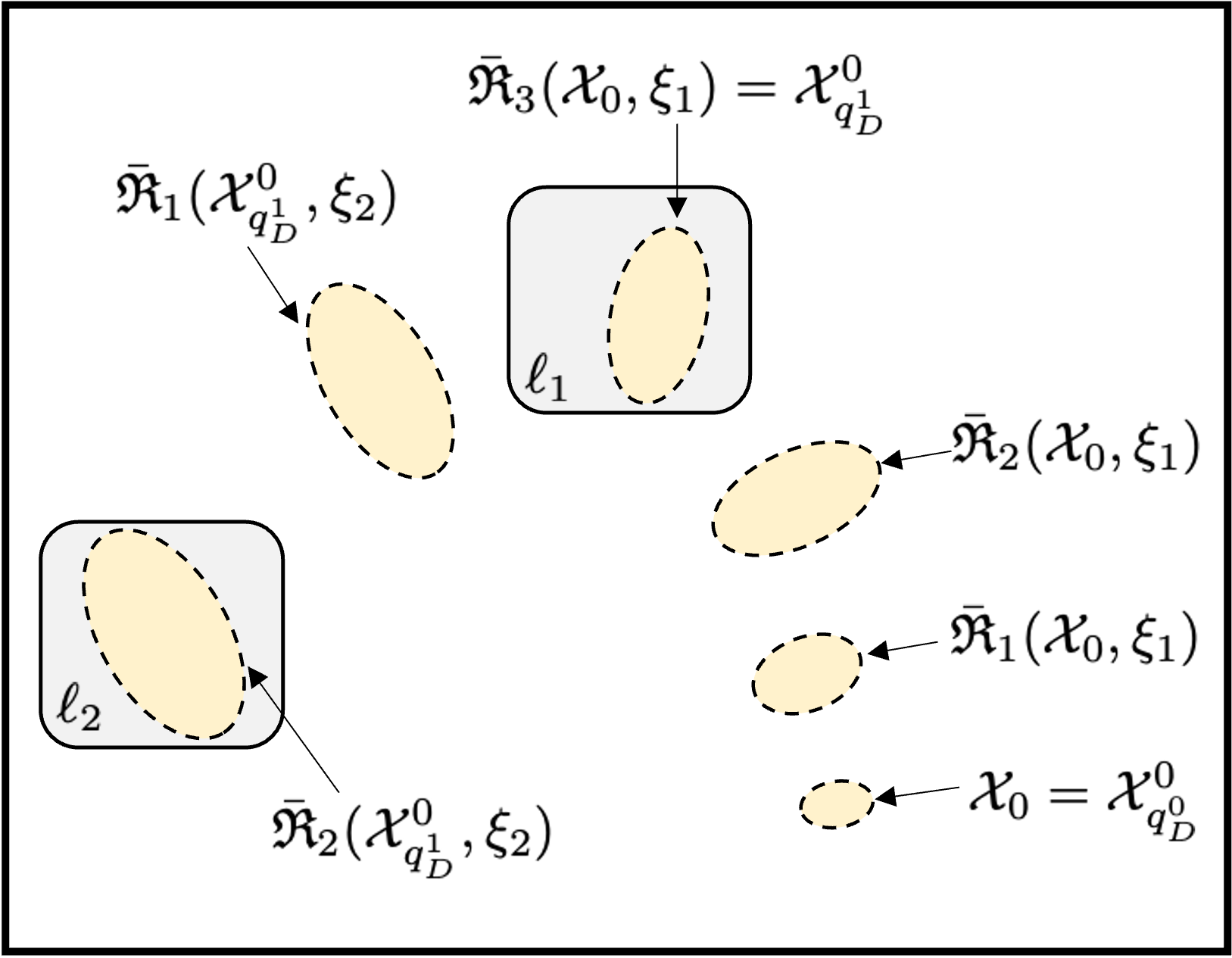
Consider the DFA in Fig. 1(a) and, specifically, the transition from to . To reach from , the available controllers are by construction of the set ; see Ex. III.2 and Section II. Let . Then, we compute reachable sets ; see Fig. 1(b). Observe that , since the sets for satisfy (5) and satisfies (6). Thus, the transition from to is verified to be safe. For the transition from to , we have that . Verification of this transition will be discussed in Ex. III.4. Finally, we have and .
III-D From Verification of Reach-Avoid Properties to Verification of LTL formulas
To verify that the system satisfies , it suffices to check that the final DFA state can be reached from the initial state by enabling a sequence of DFA transitions that are verified to be safe; see also Section III-A. To check this we rely on applying graph-search methods over the DFA state while verifying on-the-fly safety of DFA transitions using reachability analysis; see Section III-C. Specifically, first we view the DFA as a directed graph with vertices and edges that are determined by the set of states and transitions of the DFA. As discussed in Section III-C, to verify safety of DFA transition, an initial set of states is needed denoted by . This set captures all possible states in that the system may have when it reaches a DFA state . As a result, depends on the previous DFA states that the system has gone through to reach . To simplify the proposed algorithm, we pre-process so that each node in that can be reached through multiple paths (excluding self-loops) originating from is replicated so that each replica can be reached through a unique path (excluding self-loops). For each vertex , we define sets that collect its incoming and outgoing edges denoted by and , respectively. If the number of incoming edges (excluding self-loops) for is greater than , i.e., we create copies of denoted by . Each node has only one incoming edge which is selected to be the -th edge in , denoted by , while its outgoing edges remain the same as in the original node . Then we add all copies to the graph and remove the original nodes . We denote the resulting graph by .
Next, we apply a Depth-first search (DFS) method over to see if can be reached from through a sequence of DFA transitions that are verified to be safe. This process is summarized in Alg. 1. The inputs to this algorithm are the graph , the set of NN controllers and the system dynamics (1) (line 1). In what follows, we denote by the currently visited node in . The set of all possible states in that the system can be when it reaches is denoted by . We initialize as and . Also, we define a set that collects all nodes in that have been visited and a sequence of nodes that points to the current path from towards . They are initialized as and . Also we initialize the control strategy as an empty sequence. We also define a function that maps a DFA state to the corresponding set ; this function that is constructed on-the-fly is need only as way store and recover from memory the sets (lines 2-3). Given , we randomly select a next state . Then we apply reachability analysis over the transition from to using the NN controllers and the initial set of states (lines 5-6); see Section III-C. If the transition is verified to be safe, then we append to . Also, we append the controller for which this transition is safe to that denotes the current control strategy to reach from (lines 7-8). The corresponding horizon should be stored as well; we abstain from this for simplicity of presentation. The final reachable set becomes the set ; see Ex. III.4 and Fig. 1(b) as well (line 8). Also, is constructed on-the-fly as and we replace with (line 9). If the transition is not verified to be safe, we remove from the set (see (3)). Then we keep taking out the last element in and , denoted by and , while is assigned to until we find another state in that has not been not visited yet (lines 12-16). The above process is repeated until is updated to be . In this case, we have found a NN control strategy that satisfies for all initial states (line 10-11). If is empty yet we fail to find another state in that is not visited, then the proposed method cannot find a feasible path from to (even though it may exist; see Section III-E) (lines 17-18). We note that any other graph-search method in conjunction with reachability analysis can be used as well.
III-E Correctness & Completeness
Proposition III.5 (Correctness)
The proposed method is correct, i.e., the computed solves Problem 1.
Proof:
This result holds by construction of the proposed method. Particularly, we ensure that the closed-loop system (2) driven by , where each is applied for time-steps, generates trajectories , where , that satisfy the system dynamics and the LTL formula , . ∎
Remark III.6 (Computational Efficiency vs Completeness)
In general, our method is not complete in the sense that it may not find a control strategy that satisfies , for all , even though such a strategy exists. This is due to the fact that (a) Alg. 1 computes over-approximated reachable sets and that (b) it does not exhaustively search over all possible combinations of NN control actions that the system can apply when a new DFA state is reached. As for (b), for instance, given a initial set of states for , Alg. 1 reasons about safety of a transition from to , using only controllers selected from . If this transition is unsafe, then it is discarded. However, this transition may become feasible if the initial set of states changes, which can happen by applying a controller from for some time steps. Additionally, as soon as Alg. 1 finds a for which the corresponding transition is safe, it proceeds to new DFA transitions. However, that transition may be safe for other controllers in as well, where each one yields a different initial set for subsequent DFA transitions affecting their safety. The proposed method can be extended to account for these additional control actions at the expense of increasing its computational cost. We note that such trade-offs are quite common in related works; see e.g., [25]. The proposed method is complete if (i) there are no self-loops in the DFA states, or if for all states (see e.g., Ex. III.3); (ii) , for all ; (iii) the reachable sets are accurately computed.
IV Experiments
In this section, we demonstrate our framework on an unmanned aerial vehicle (UAV) with various LTL properties.
System Dynamics: We consider a UAV with dynamics as in (1) where the matrices and are defined as in [8]. The UAV state is defined as capturing the position and velocity. The control input is a function of pitch, roll and thrust.
NN controllers: In what follows, we define LTL specifications that require the UAV to visit certain disjoint regions of interest . We highlight that the the regions are defined only over the UAV position, i.e., . Also, since we assume disjoint regions, the DFA can be pruned by removing infeasible DFA transitions reducing the computational cost for verification [20]. We train the NN controllers similarly to [8]; nevertheless, any other method (e.g., RL) can be used to train them. Specifically, to train , we leverage nonlinear Model Predictive Control (MPC) methods. First we generate a random set of states . Starting from each one of these states, we generate a sequence of pairs of states and control inputs that drive the UAV towards the interior of using an off-the-shelf MPC solver [26]. Each pair constitutes a data point in a training dataset. Using this dataset we train feedforward NN controllers with hidden layers, neurons/layer, and ReLU activation functions.


Case Study I: In this case study, we consider the following LTL formula requiring the UAV to eventually visit the regions and , in any order, while avoiding the obstacles and . This formula corresponds to the DFA shown in Fig. 2(a); notice that the transition from to was pruned and, therefore, not considered during verification since it requires the UAV to be present in more than one region simultaneously. To train and we collected datapoints for each controller. Given these trained NN controllers and an initial set of states defined as an ellipsoid centered at with shape matrix of . We check if there exists a sequence of control actions that satisfy . Particularly, first it investigates the DFA transition from to . This transition requires the UAV to stay within the obstacle-free space (i.e., avoid the obstacles and ) and eventually reach . The corresponding reachable sets for this DFA transition are shown in Figure 3(a). Notice that the reachable sets are fully outside the obstacle regions for while at the corresponding reachable set is fully inside . Thus, this DFA transition is verified to be safe. Next, the DFA transition from to is considered requiring the robot to reach while avoiding the obstacle regions. The set of initial states for this transition is . After computing reachable sets (not shown), we can see that for they are outside the obstacles while is inside verifying that this DFA transition is also safe. Thus, there exists a control strategy where such that for all .


Case Study II: In this case study, we consider an LTL formula requiring the UAV to eventually visit either region or , while avoiding obstacles and . This formula corresponds to the DFA shown in Figure 2(b). The NN controller is the same as in the previous case study while was trained using only datapoints to mimic a poorly designed controller. The initial set of states is defined as an ellipsoid centered at with shape matrix of . Given the DFA, we investigate the transition from to which requires the UAV to reach either or while avoiding both and . In other words, we have that and . Thus, we have that . First, we check if this DFA transition is safe using . The generated reachable sets are shown in Figure 3(b); only the first reachable sets are shown. We observed that could not be reached within a large enough number of iterations. Thus, we cannot reason about safety of this DFA transition under . Thus, next we consider the controller and we constructed the sets (not shown) demonstrating that all obstacles are avoided while at the the reachable set is fully inside . Thus, we verify that there exists , where is applied for steps, so that , for all .

Case Study III: We revisit the LTL formula considered in Ex. III.2-III.4 with DFA shown in Fig. 1(a). The controllers and are the same as in case study I while is defined as an ellipsoid centered at with shape matrix of . To check whether the DFA transition from to is safe, we check if the system can reach while avoiding . By constructing the reachable sets, we notice that cannot be reached without entering first; see Fig. 4. Thus, we cannot find a for ; see Rem. III.6.
V Conclusion
This paper proposed a new method to design verified compositions of NN controllers for co-safe LTL tasks. We showed its efficiency in navigation tasks for aerial vehicles.
References
- [1] Q. Gao, D. Hajinezhad, Y. Zhang, Y. Kantaros, and M. M. Zavlanos, “Reduced variance deep reinforcement learning with temporal logic specifications,” in 10th ACM/IEEE International Conference on Cyber-Physical Systems, 2019, pp. 237–248.
- [2] V. Rubies-Royo, D. Fridovich-Keil, S. Herbert, and C. J. Tomlin, “A classification-based approach for approximate reachability,” in 2019 International Conference on Robotics and Automation (ICRA). IEEE, 2019, pp. 7697–7704.
- [3] S. Huang, N. Papernot, I. Goodfellow, Y. Duan, and P. Abbeel, “Adversarial attacks on neural network policies,” arXiv preprint arXiv:1702.02284, 2017.
- [4] M. Fazlyab, M. Morari, and G. J. Pappas, “Safety verification and robustness analysis of neural networks via quadratic constraints and semidefinite programming,” IEEE Trans on Automatic Control, 2020.
- [5] S. Dutta, S. Jha, S. Sankaranarayanan, and A. Tiwari, “Output range analysis for deep feedforward neural networks,” in NASA Formal Methods Symposium. Springer, 2018, pp. 121–138.
- [6] C. Huang, J. Fan, W. Li, X. Chen, and Q. Zhu, “Reachnn: Reachability analysis of neural-network controlled systems,” ACM Transactions on Embedded Computing Systems (TECS), vol. 18, no. 5s, pp. 1–22, 2019.
- [7] X. Sun, H. Khedr, and Y. Shoukry, “Formal verification of neural network controlled autonomous systems,” in International Conference on Hybrid Systems: Computation and Control, 2019, pp. 147–156.
- [8] H. Hu, M. Fazlyab, M. Morari, and G. J. Pappas, “Reach-sdp: Reachability analysis of closed-loop systems with neural network controllers via semidefinite programming,” 59th IEEE Conference on Decision and Control (CDC), pp. 5929–5934, December 2020.
- [9] H.-D. Tran, X. Yang, D. M. Lopez, P. Musau, L. V. Nguyen, W. Xiang, S. Bak, and T. T. Johnson, “NNV: The neural network verification tool for deep neural networks and learning-enabled cyber-physical systems,” Computer Aided Verification, vol. 12224, pp. 3 – 17, 2020.
- [10] S. Dutta, X. Chen, and S. Sankaranarayanan, “Reachability analysis for neural feedback systems using regressive polynomial rule inference,” in Proceedings of the 22nd ACM International Conference on Hybrid Systems: Computation and Control, 2019, pp. 157–168.
- [11] R. Ivanov, T. Carpenter, J. Weimer, R. Alur, G. Pappas, and I. Lee, “Verisig 2.0: Verification of neural network controllers using taylor model preconditioning,” in International Conference on Computer Aided Verification. Springer, 2021, pp. 249–262.
- [12] S. Sun, Y. Zhang, X. Luo, P. Vlantis, M. Pajic, and M. M. Zavlanos, “Formal verification of stochastic systems with relu neural network controllers,” in 2022 International Conference on Robotics and Automation (ICRA). IEEE, 2022, pp. 6800–6806.
- [13] K. Jothimurugan, S. Bansal, O. Bastani, and R. Alur, “Compositional reinforcement learning from logical specifications,” Advances in Neural Information Processing Systems, vol. 34, 2021.
- [14] G. N. Tasse, D. Jarvis, S. James, and B. Rosman, “Skill machines: Temporal logic composition in reinforcement learning,” arXiv preprint arXiv:2205.12532, 2022.
- [15] C. Neary, C. Verginis, M. Cubuktepe, and U. Topcu, “Verifiable and compositional reinforcement learning systems,” in Proceedings of the International Conference on Automated Planning and Scheduling, vol. 32, 2022, pp. 615–623.
- [16] R. Ivanov, K. Jothimurugan, S. Hsu, S. Vaidya, R. Alur, and O. Bastani, “Compositional learning and verification of neural network controllers,” ACM Trans. Embed. Comput. Syst., vol. 20, no. 5s, sep 2021. [Online]. Available: https://doi.org/10.1145/3477023
- [17] C. Baier and J.-P. Katoen, Principles of model checking. MIT press Cambridge, 2008, vol. 26202649.
- [18] S. W. Chen, T. Wang, N. Atanasov, V. Kumar, and M. Morari, “Large scale model predictive control with neural networks and primal active sets,” Automatica, vol. 135, p. 109947, 2022.
- [19] K. Leahy, D. Zhou, C.-I. Vasile, K. Oikonomopoulos, M. Schwager, and C. Belta, “Persistent surveillance for unmanned aerial vehicles subject to charging and temporal logic constraints,” Autonomous Robots, vol. 40, no. 8, pp. 1363–1378, 2016.
- [20] Y. Kantaros and M. M. Zavlanos, “Stylus*: A temporal logic optimal control synthesis algorithm for large-scale multi-robot systems,” International Journal of Robotics Research, 2020.
- [21] E. M. Hahn, M. Perez, S. Schewe, F. Somenzi, A. Trivedi, and D. Wojtczak, “Omega-regular objectives in model-free reinforcement learning,” TACAS, 2018.
- [22] Y. Kantaros, “Accelerated reinforcement learning for temporal logic control objectives,” in IEEE/RSJ International Conference on Intelligent Robots and Systems, Kyoto, Japan, October 2022.
- [23] A. K. Bozkurt, Y. Wang, M. M. Zavlanos, and M. Pajic, “Control synthesis from linear temporal logic specifications using model-free reinforcement learning,” in 2020 IEEE International Conference on Robotics and Automation (ICRA). IEEE, 2020, pp. 10 349–10 355.
- [24] F. Fuggitti, “Ltlf2dfa,” March 2019. [Online]. Available: https://github.com/whitemech/LTLf2DFA
- [25] K. Leahy, A. Jones, and C. I. Vasile, “Fast decomposition of temporal logic specifications for heterogeneous teams,” IEEE Robotics and Automation Letters, 2022.
- [26] N. Andrei, “A sqp algorithm for large-scale constrained optimization: Snopt,” in Continuous nonlinear optimization for engineering applications in GAMS technology. Springer, 2017, pp. 317–330.