跳到论文正文
W Papers独立论文阅读器 arXiv:2209.05854 论文正文 计算阅读时间 · 0%
引用这篇论文根据当前论文元数据生成,正式投稿前建议核对。


License: CC Zero
arXiv:2209.05854v2 [math.CV] 06 Aug 2023

Overcrowding for zeros of Hyperbolic Gaussian analytic functions

Keren Mor Waknin Address: School of Mathematical Sciences, Tel Aviv University, Tel Aviv 69978, Israel Email address: kerenmor22@gmail.com
Abstract.

We consider the family {fL}L>0\{f_{L}\}_{L>0} of Gaussian analytic functions in the unit disk, distinguished by the invariance of their zero set with respect to hyperbolic isometries. Let nL​(r)n_{L}\left(r\right) be the number of zeros of fLf_{L} in a disk of radius rr. We study the asymptotic probability of the rare event where there is an overcrowding of the zeros as r↑1r\uparrow 1, i.e. for every L>0L>0, we are looking for the asymptotics of the probability ℙ[nL(r)≥V(r)]\mathbb{P}\left[n_{L}(r)\geq V(r)\right] with V⁡(r)V\left(r\right) large compared to the 𝔼​[nL​(r)]\mathbb{E}\left[n_{L}\left(r\right)\right]. Peres and Virág showed that for L=1L=1 (and only then) the zero set forms a determinantal point process, making many explicit computations possible. Curiously, contrary to the much better understood planar model, it appears that for L<1L<1 the exponential order of decay of the probability of overcrowding when VV is close to 𝔼​[nL​(r)]\mathbb{E}\left[n_{L}\left(r\right)\right] is much less than the probability of a deficit of zeros.

1. Introduction

We study hyperbolic Gaussian analytic functions (GAFs) in the unit disk 𝔻\mathbb{D}

fL​(z)=∑n≥0ξn​L(L+1)⋯(L+n−1)n!​zn,for​L>0,f_{L}\left(z\right)=\sum_{n\geq 0}\xi_{n}\sqrt{\frac{L\left(L+1\right)\cdots\left(L+n-1\right)}{n!}}z^{n},\quad\text{for}\ L>0,

where {ξn}n≥0\{\xi_{n}\}_{n\geq 0} are independent standard complex Gaussian random variables. The zero set of this family has a distinguished property, which is the invariance of the distribution of their zero set 𝒵f=f−1​{0}\mathcal{Z}_{f}=f^{-1}\{0\} with respect to Möbius transformations of the unit disk. This property is unique in the sense that these are the only GAFs, up to a multiplication by a deterministic nowhere vanishing analytic function, whose zeros are isometry-invariant under the respective group of isometries [9, Chap. 2]. Let nL​(r)=#⁡{z:f⁡(z)=0​and​|z|≤r}n_{L}\left(r\right)=\#\{z\ :\ f\left(z\right)=0\ \text{and}\ \left|z\right|\leq r\} be the number of zeros of fLf_{L} in the disk of radius r∈(0,1)r\in\left(0,1\right). Because of the invariant distribution of the zero set, the first intensity is equal to a constant multiple of the hyperbolic measure on the unit disk. In fact, it is not hard to check that

(1) 𝔼​[nL​(r)]=L​r21−r2\mathbb{E}[n_{L}(r)]=\frac{Lr^{2}}{1-r^{2}}

see [18]. Buckley [1] studied the asymptotic of the variance vL​(r)v_{L}\left(r\right) and proved that there is a transition in the asymptotics of the variance at L=12L=\frac{1}{2}. The case L=1L=1 is special in the hyperbolic models. Peres and Virág [17] discovered that the zero set of the Gaussian Taylor series f1​(z)=∑n=0∞ξn​znf_{1}(z)=\sum_{n=0}^{\infty}\xi_{n}z^{n} is a determinantal point process, which allowed them to directly compute a lot of its characteristics (see [9, Chapter 4] and also [9, Section 5.1]). Peres and Virág also showed that L=1L=1 is the only instance when the zero set of fLf_{L} is a determinantal point process. In [3] Buckley, Nishry, Peled, and Sodin found the rate of decay of the hole probability pH(r):=ℙ[{fL≠0onr𝔻¯}]p_{H}\left(r\right):=\mathbb{P}\left[\{f_{L}\neq 0\ \text{on}\ r\bar{\mathbb{D}}\}\right] as r↑1r\uparrow 1. Recently, Buckley and Nishry [2] proved that the limiting (in law) behavior of the normalized version of nL​(r)n_{L}\left(r\right):

n^L​(r):=nL​(r)−𝔼⁡[nL​(r)]vL​(r),r↑1,\widehat{n}_{L}\left(r\right):=\frac{n_{L}\left(r\right)-\mathbb{E}\left[n_{L}\left(r\right)\right]}{\sqrt{v_{L}\left(r\right)}},\quad r\uparrow 1,

has a transition when L=12L=\frac{1}{2}. They showed that nL​(r)n_{L}\left(r\right) satisfies a CLT for L≥12L\geq\frac{1}{2} and exhibits non-Gaussian limiting behavior for L<12L<\frac{1}{2}. The case L=1L=1 was treated previously by Peres and Virág [17]. For the hyperbolic Gaussian analytic functions Krishnnapur [11] found some bounds for the probability of the overcrowding event {nL(r)≥m}\{n_{L}\left(r\right)\geq m\} with rr fixed as m→∞m\rightarrow\infty. In this work we give matching lower and upper bounds for the overcrowding probability when r↑1r\uparrow 1 (see Theorem 1.2).

The first result is about large deviations in the case L=1L=1.

Theorem 1.1.

Let μr,v1​(r)\mu_{r},v_{1}\left(r\right) be the expectation and the variance of n1​(r)n_{1}\left(r\right) respectively. Then, for r↑1r\uparrow 1,

−logℙ[|n1(r)−μr|≥t⋅v1(r)α]∼c(t)v1(r)2​α−1-\log\mathbb{P}\left[\left|n_{1}(r)-\mu_{r}\right|\geq t\cdot v_{1}\left(r\right)^{\alpha}\right]\sim c(t)v_{1}(r)^{2\alpha-1}

where

c⁡(t)={t2212<α<1,12​(t+2)2+2​Li2⁡(1−exp⁡(t+22+W0​(−t+22​et+22)))+(t+2)​W0​(−t+22​et+22)α=1,t24α>1,c(t)=\begin{cases}{\frac{t^{2}}{2}}&\frac{1}{2}<\alpha<1,\\ \tfrac{1}{2}\left(t+2\right)^{2}+2\Li_{2}\left(1-\exp\left(\frac{t+2}{2}+W_{0}\left(-\frac{t+2}{2e^{\frac{t+2}{2}}}\right)\right)\right)+\left(t+2\right)W_{0}\left(-\frac{t+2}{2e^{\frac{t+2}{2}}}\right)&\alpha=1,\\ {\frac{t^{2}}{4}}&\alpha>1,\end{cases}

Li2(z)=−∫0zlog⁡(1−u)udu\Li_{2}(z)=-\int_{0}^{z}\frac{\log(1-u)}{u}du is the dilogarithm function [12], and W0W_{0} is the principal branch of the Lambert WW function [4].

We prove Theorem 1.1 in Appendix A. Our second result is the asymptotics of the overcrowding probability for general L>0L>0.

Theorem 1.2.

Fix L>0L>0. Then there exists CL>0C_{L}>0 such that for all r∈[12,1)r\in\left[\tfrac{1}{2},1\right) and all V>1V>1 satisfying

V≥CL1−r​log⁡11−r,V\geq\frac{C_{L}}{1-r}\log\frac{1}{1-r},

we have

−logℙ[nL(r)≥V]≃L(1−r)V2.-\log\mathbb{P}\left[n_{L}(r)\geq V\right]\simeq_{L}\left(1-r\right)V^{2}.
Corollary 1.3.

For all L>0L>0 and α>1\alpha>1 we get as r↑1r\uparrow 1,

−logℙ[nL(r)≥vL(r)α]≃L,α{(11−r)2​α−1L>12,(11−r)2​α−1​log2​α⁡(11−r)L=12,(11−r)2​α​(2−2​L)−10<L<12.-\log\mathbb{P}\left[n_{L}(r)\geq v_{L}\left(r\right)^{\alpha}\right]\simeq_{L,\alpha}\begin{cases}\left(\frac{1}{1-r}\right)^{2\alpha-1}&L>\frac{1}{2},\\ \left(\frac{1}{1-r}\right)^{2\alpha-1}\log^{2\alpha}\left(\frac{1}{1-r}\right)&L=\frac{1}{2},\\ \left(\frac{1}{1-r}\right)^{2\alpha(2-2L)-1}&0<L<\frac{1}{2}.\end{cases}

1.1. Related works

1.1.1. Comparison with the Gaussian entire function (GEF)

An analogue process to fLf_{L} whose zero set distribution is invariant under isometries of the plane is given by

gL​(z)=∑n≥0ξn​Lnn!​zn.g_{L}\left(z\right)=\sum_{n\geq 0}\xi_{n}\sqrt{\frac{L^{n}}{n!}}z^{n}.

with L>0L>0. Note that it is enough to consider the case L=1L=1 since other values of LL are just scaled versions of this case (unlike the hyperbolic model). The mean number of zeros is equal to Lπ\frac{L}{\pi}, with respect to the Lebesgue measure d​m​(z)dm\left(z\right) on the plane. The asymptotics of the variance in the planar v⁡(R)v\left(R\right) was computed by Forrester and Honner in [7]:

v⁡(R)=c​R+o⁡(R),R→∞.v\left(R\right)=cR+o\left(R\right),\quad R\rightarrow\infty.

We use upper case RR for the radius to emphasize that the function’s domain is ℂ\mathbb{C}. In [1], Buckley proved that for the hyperbolic model the asymptotic of the variance is given by:

vL​(r)∼{cL1−rfor ​L>12,c1−r​log⁡11−rfor​L=12,cL(1−r)2−2​Lfor ​0<L<12,​r→1−,v_{L}\left(r\right)\sim\begin{cases}\frac{c_{L}}{1-r}&\text{for }\ L>\frac{1}{2},\\ \frac{c}{1-r}\log\frac{1}{1-r}&\text{for}\ L=\frac{1}{2},\\ \frac{c_{L}}{(1-r)^{2-2L}}&\text{for }0<L<\frac{1}{2},\end{cases}r\rightarrow 1^{-},

where the constants are explicitly computed and positive in all three cases. Note that in the planar case, the expectation 𝔼⁡[n⁡(R)]\mathbb{E}\left[n\left(R\right)\right] is in fact the Lebesgue measure of the disc with radius RR, which is much larger (by factor of RR) than the variance v⁡(R)v\left(R\right), which is proportional to the length of the boundary of the disc. However, in the hyperbolic case, the hyperbolic area and the length circumference of a disk of radius rr are approximately the same and contrary to the plane, the variance is greater or equal (up to constants) than the expectation (1) (depending on the values of LL). It is also quite natural to study the probability of (large) fluctuations. We will restrict ourselves to the case of a disk with large radius rr with respect to the function’s domain (i.e in the unit disk rr is close to 1 and in the complex plane RR tends to infinity) and study the probability:

ℙ[|nL(r)−𝔼[nL(r)]|≥vL(r)α],\mathbb{P}\left[\left|n_{L}\left(r\right)-\mathbb{E}\left[n_{L}\left(r\right)\right]\right|\geq v_{L}\left(r\right)^{\alpha}\right],

beyond what is known by asymptotic normality (i.e. α>12\alpha>\frac{1}{2}). This might be called moderate\\backslashlarge\\backslashhuge deviations in probability language, depending on α\alpha and the model we consider. For the GEF there is a complete answer in terms of α\alpha given by:

Theorem 1.4 (Jancovici-Lebowitz-Manificat Law [14, 11, 19]).

As R→∞R\rightarrow\infty

log(−log(ℙ[|n(R)−R2|>Rα]))log⁡R→{2​α−112≤α≤1,3​α−21≤α≤2,2​αα≥2.\frac{\log\left(-\log\left(\mathbb{P}\left[\left|n\left(R\right)-R^{2}\right|>R^{\alpha}\right]\right)\right)}{\log R}\rightarrow\begin{cases}2\alpha-1&\frac{1}{2}\leq\alpha\leq 1,\\ 3\alpha-2&1\leq\alpha\leq 2,\\ 2\alpha&\alpha\geq 2.\end{cases}

Here we can see that the asymptotic behavior changes for different values of the exponent α\alpha, unlike the case of the hyperbolic GAF Theorem 1.1. i.e. considering the log⁡log\log\log asymptotic of this probability as r↑1r\uparrow 1, it holds that the power remains 2​α−12\alpha-1.

1.1.2. Determinantal point processes in the unit disk

Our result for the determinantal process in the hyperbolic model is related to recent work of Fenzl and Lambert (see [6]), where they compute the precise deviations for disk counting statistic of rotation invariant determinantal point processes in the disk and the plane. In particular they proved that the large deviations principle holds for the determinantal point process (L=1L=1) and provided a general formula for the rate of decay in terms of the rate function. Here we provide an explicit expression to the rate function. Since the only case when the hyperbolic GAF form a determinantal point process is when L=1L=1, we need to use other techniques for different values of LL.

1.1.3. Overcrowding estimates.

In [11] Krishnapur studied the overcrowding probability for zeros of the hyperbolic GAF. Our lower bound for ℙ[nL(r)≥V]\mathbb{P}\left[n_{L}\left(r\right)\geq V\right] is close to his. Our upper bound is more precise, mainly because we found a more accurate estimate of the asymptotic probability

ℙ[∫r​𝕋log|f(rei​θ)|dμ≤−x],asx→∞.\mathbb{P}\left[\int_{r\mathbb{T}}\log|f(re^{i\theta})|d\mu\leq-x\right],\qquad\text{as}\ \,x\to\infty.

Krishnapur conjectured that his lower bound gives the correct order of decay of the overcrowding probability, and our Theorem 1.2 confirms his conjecture.

1.1.4. Hole probability

Consider the event when f⁡(z)≠0f\left(z\right)\neq 0 in r​𝔻r\mathbb{D}, sometimes called the hole event. We denote pH(r):=ℙ[{fL≠0onr𝔻¯}]p_{H}\left(r\right):=\mathbb{P}\left[\{f_{L}\neq 0\ \text{on}\ r\bar{\mathbb{D}}\}\right] and are interested in its decay as R→∞R\rightarrow\infty or r→1−r\rightarrow 1^{-}. There are results regarding the rate of decay of the hole probability in both models - the planar and the hyperbolic:

Theorem 1.5 ([15],[8],[19]).

Suppose R→∞R\rightarrow\infty. Then,

−log⁡pH​(R)=e24​R4+O⁡(R2​log2​R).-\log p_{H}\left(R\right)=\frac{e^{2}}{4}R^{4}+O\left(R^{2}\log^{2}R\right).
Theorem 1.6 ([3, Theorem 1]).

Suppose r↑1r\uparrow 1. Then,

−logpH(r)≃L{1(1−r)L​log⁡11−rfor ​ 0<L<1,11−r​log⁡11−rfor​L=1,11−r​log2​11−rfor ​L>1,r→1−,-\log p_{H}(r)\simeq_{L}\begin{cases}\frac{1}{\left(1-r\right)^{L}}\log\frac{1}{1-r}&\text{for }\ 0<L<1,\\ \frac{1}{1-r}\log\frac{1}{1-r}&\text{for}\ L=1,\\ \frac{1}{1-r}\log^{2}\frac{1}{1-r}&\text{for }L>1,\end{cases}r\rightarrow 1^{-},

where the constants are explicitly computed and positive.

1.1.5. Loss of the balance between excess of zeros and their deficit.

Consider the event of excess of zeros where {nL(r)>μr+vL(r)}\{n_{L}\left(r\right)>\mu_{r}+v_{L}\left(r\right)\} and the event of deficit of zeroes {nL(r)<μr−vL(r)}\{n_{L}\left(r\right)<\mu_{r}-v_{L}\left(r\right)\} where μr=𝔼⁡[nL​(r)]\mu_{r}=\mathbb{E}\left[n_{L}\left(r\right)\right]. Heuristically, letting α↓1\alpha\downarrow 1 in Theorem 1.2 would imply

−logℙ[nL(r)>μr+vL(r)α]≃−logℙ[nL(r)>vL(r)α]\displaystyle-\log\mathbb{P}\left[n_{L}\left(r\right)>\mu_{r}+v_{L}\left(r\right)^{\alpha}\right]\simeq-\log\mathbb{P}\left[n_{L}\left(r\right)>v_{L}\left(r\right)^{\alpha}\right] ≃vL​(r)2​α−1\displaystyle\simeq v_{L}\left(r\right)^{2\alpha-1}
∼α↓1​{vL​(r)12≤L<1,vL​(r)3−4​L2−2​L0<L<12,\displaystyle\overset{\alpha\downarrow 1}{\sim}\begin{cases}v_{L}\left(r\right)&\frac{1}{2}\leq L<1,\\ v_{L}\left(r\right)^{\frac{3-4L}{2-2L}}&0<L<\frac{1}{2},\end{cases}

while the hole probability results implies that

−logℙ[nL(r)<μr−vL(r)α]\displaystyle-\log\mathbb{P}\left[n_{L}\left(r\right)<\mu_{r}-v_{L}\left(r\right)^{\alpha}\right] ≥1(1−r)L​log⁡11−r≃{vL​(r)L,12≤L<1,vL​(r)L2−2​L,0<L<12\displaystyle\geq\frac{1}{\left(1-r\right)^{L}}\log\frac{1}{1-r}\simeq\begin{cases}v_{L}\left(r\right)^{L},&\frac{1}{2}\leq L<1,\\ v_{L}\left(r\right)^{\frac{L}{2-2L}},&0<L<\frac{1}{2}\end{cases}

up to some logarithmic factor which we neglect. I.e. the exponent is different and we do not get the symmetry between these events (contrary to the planar model), the probability for deficit is bigger.

1.2. Notation & Some special functions

  • –

    cc and CC denote positive numerical constants that do not depend on r,α,Lr,\alpha,L. By cLc_{L} we denote positive constant that depends only on LL. In this work, the values of these constants are irrelevant and may vary from line to line.

  • –

    The notation X≃YX\simeq Y means that there exists positive constants such that c​X≤Y≤C​XcX\leq Y\leq CX. The notation X≃LYX\simeq_{L}Y is used when the constants depend on LL.

  • –

    e⁡(t)=e2​π​i​te\left(t\right)=e^{2\pi it}.

  • –

    [x]\left[x\right] denotes the integer part of xx.

  • –

    n≡k⁡(N)n\equiv k\left(N\right) means that n≡k​modulo​Nn\equiv k\ \text{modulo}\ N.

  • –

    r​𝔻r\mathbb{D} denotes the open disk {z:|z|<r}\{z:|z|<r\} and r​𝕋r\mathbb{T} denotes its boundary {z:|z|=r}\{z:|z|=r\}.

  • –

    The planar Lebesgue measure is denoted by mm and the normalized angular measure on r​𝕋r\mathbb{T} is denoted by μ\mu.

  • –

    We set δ:=1−r\delta:=1-r. We always assume that rr is sufficiently close to 11 (and hence δ\delta close to 00).

  • –

    Let f⁡(r),g⁡(r)f\left(r\right),g\left(r\right) be positive functions. The notation f⁡(r)∼g⁡(r)f\left(r\right)\sim g\left(r\right) as r↑1r\uparrow 1 means that limr↑1f⁡(r)g⁡(r)=1\lim_{r\uparrow 1}\frac{f\left(r\right)}{g\left(r\right)}=1. The notation f⁡(r)≪g⁡(r)f\left(r\right)\ll g\left(r\right) as r↑1r\uparrow 1 means that limr↑1f⁡(r)g⁡(r)=0\lim_{r\uparrow 1}\frac{f\left(r\right)}{g\left(r\right)}=0.

Acknowledgments

I am deeply grateful to my MSc advisors, Alon Nishry and Mikhail Sodin, for their constant encouragement, endless patience and enlightening discussions throughout this project. I would also like to thank Naomi Feldheim, Manjunath Krishnapur, Ron Peled and Oren Yakir for their valuable comments and fruitful discussions. I thank Lakshmi Priya for reading this paper with great care and making very insightful comments, which improved both the mathematics and the presentation. I thank the referee for careful reading this work and several useful suggestions. This work was supported by ERC Advanced Grant 692616, ISF Grant 382/15 and by BSF Start up Grant no. 2018341.

2. Proof of Theorem 1.2

Fix L>0L>0. Recall that we want to prove that there exists CL>0C_{L}>0 such that for all r∈[12,1)r\in\left[\tfrac{1}{2},1\right) and all V>1V>1 satisfying

(2) V≥CL1−r​log⁡11−r,V\geq\frac{C_{L}}{1-r}\log\frac{1}{1-r},

we have

−logℙ[nL(r)≥V]≃L(1−r)V2.-\log\mathbb{P}\left[n_{L}(r)\geq V\right]\simeq_{L}\left(1-r\right)V^{2}.

Several remarks on Theorem 1.2

  1. (1)

    Assumption (2) is meant to ensure that the number of zeros VV is large enough (compared with the expectation).

  2. (2)

    Recall that

    vL​(r)=Var​[nL​(r)]∼{cL1−rfor ​L>12,c1−r​log⁡11−rfor​L=12,cL(1−r)2−2​Lfor ​0<L<12,r↑1.v_{L}\left(r\right)=\textrm{Var}\left[n_{L}\left(r\right)\right]\sim\begin{cases}\frac{c_{L}}{1-r}&\text{for }\ L>\frac{1}{2},\\ \frac{c}{1-r}\log\frac{1}{1-r}&\text{for}\ L=\frac{1}{2},\\ \frac{c_{L}}{(1-r)^{2-2L}}&\text{for }0<L<\frac{1}{2}\end{cases}\quad,\quad r\uparrow 1.

    By the above, vLα​(r)v_{L}^{\alpha}\left(r\right) will satisfy assumption (2), provided that either L>0L>0, α>1\alpha>1, or L<12L<\frac{1}{2}, α∈(12−2​L,1]\alpha\in(\frac{1}{2-2L},1]. In both cases vL​(r)α≫μr=L​r21−r2v_{L}(r)^{\alpha}\gg\mu_{r}=\frac{Lr^{2}}{1-r^{2}} as r↑1r\uparrow 1, and hence

    logℙ[|nL(r)−μr|≥vL(r)α]≃logℙ[nL(r)≥vL(r)α].\log\mathbb{P}\left[\left|n_{L}(r)-\mu_{r}\right|\geq v_{L}\left(r\right)^{\alpha}\right]\simeq\log\mathbb{P}\left[n_{L}\left(r\right)\geq v_{L}\left(r\right)^{\alpha}\right].

In order to prove Theorem 1.2 we find matching lower and upper bounds for the (log)(\log) probability of the overcrowding event. We employ strategies somewhat similar to the ones introduced in [11, 19, 3, 16]. Throughout the proof we will assume that rr is sufficiently close to 11, as we can do.

2.1. Lower Bound

Claim 2.1.

For r∈[12,1)r\in[\tfrac{1}{2},1) we have

logℙ[nL(r)≥V]≥−cL(1−r)V2.\log\mathbb{P}\left[n_{L}\left(r\right)\geq V\right]\geq-c_{L}\left(1-r\right)V^{2}.
Proof.

Fix rr close to 1 and take m=m⁡(r)=[V]+1m=m\left(r\right)=\left[V\right]+1. Consider the following independent events:

  • •

    E1≔{|ξn|≤n,n≥2​m+1},E_{1}\coloneqq\left\{\left|\xi_{n}\right|\leq\sqrt{n}\ ,\ n\geq 2m+1\right\},

  • •

    E2≔{|ξn|(−Ln)12≤(−Lm)12rm,m+1≤n≤2m},E_{2}\coloneqq\left\{\left|\xi_{n}\right|\binom{-L}{n}^{\frac{1}{2}}\leq\binom{-L}{m}^{\frac{1}{2}}r^{m}\ ,\ m+1\leq n\leq 2m\right\},

  • •

    E3≔{|ξm|≥4m1−r},E_{3}\coloneqq\left\{\left|\xi_{m}\right|\geq 4m\sqrt{1-r}\right\},

  • •

    E4≔{|ξn|(−Ln)12rn≤1−r(−Lm)12rm, 0≤n≤m−1}E_{4}\coloneqq\left\{\left|\xi_{n}\right|\binom{-L}{n}^{\frac{1}{2}}r^{n}\leq\sqrt{1-r}\binom{-L}{m}^{\frac{1}{2}}r^{m}\ ,\ 0\leq n\leq m-1\right\}.

Claim 2.2.

Under the events E1,E2,E3,E4E_{1},E_{2},E_{3},E_{4}, on |z|=r|z|=r we have,

|fL​(z)−ξm​(−Lm)12​zm|<|ξm​(−Lm)12​zm|\left|f_{L}(z)-\xi_{m}\binom{-L}{m}^{\frac{1}{2}}z^{m}\right|<\left|\xi_{m}\binom{-L}{m}^{\frac{1}{2}}z^{m}\right|

whence , nL​(r)=mn_{L}\left(r\right)=m.

Claim 2.3.

For all 1≤j≤41\leq j\leq 4,

ℙ⁡[Ej]≥exp⁡(−cL​(1−r)​V2).\mathbb{P}\left[E_{j}\right]\geq\exp\left(-c_{L}\left(1-r\right)V^{2}\right).

Overall, using the independence of these events we get the desired lower bound, proving 2.1. It remains to prove these two claims.

Proof of 2.2.

It holds that

|fL​(z)−ξm​(−Lm)12​zm|\displaystyle\left|f_{L}\left(z\right)-\xi_{m}\binom{-L}{m}^{\frac{1}{2}}z^{m}\right| ≤(∑n=0m−1+∑n=m+12​m+∑n=2​m+1∞)|ξn|(−Ln)12rn\displaystyle\leq\left(\sum_{n=0}^{m-1}+\sum_{n=m+1}^{2m}+\sum_{n=2m+1}^{\infty}\right)\left|\xi_{n}\right|\binom{-L}{n}^{\frac{1}{2}}r^{n}
≤m​1−r​(−Lm)12​rm+(−Lm)12​rm⋅rm+1​(1−rm)1−r\displaystyle\leq m\sqrt{1-r}\binom{-L}{m}^{\frac{1}{2}}r^{m}+\binom{-L}{m}^{\frac{1}{2}}r^{m}\cdot\frac{r^{m+1}(1-r^{m})}{1-r}
+∑n=2​m+1∞n(−Ln)12rn.\displaystyle+\sum_{n=2m+1}^{\infty}\sqrt{n}\binom{-L}{n}^{\frac{1}{2}}r^{n}.

So we need to show that the second and the third terms on the right hand side are also bounded by m​1−r​(−Lm)12​rmm\sqrt{1-r}\binom{-L}{m}^{\frac{1}{2}}r^{m}.

  • –

    2nd term:

    rm=e−m​|log⁡r|≪1−r(assumption (2))r^{m}=e^{-m\left|\log r\right|}\ll\sqrt{1-r}\quad\text{(assumption \eqref{assumption})}

    whence,

    rm+1​1−rm1−r<m​rm≪m​1−r.r^{m+1}\frac{1-r^{m}}{1-r}<mr^{m}\ll m\sqrt{1-r}.
  • –

    3rd term: Let cn=n​(−Ln)12​rnc_{n}=\sqrt{n}\binom{-L}{n}^{\frac{1}{2}}r^{n}. Then cn+1cn=L+nn⋅r→r\frac{c_{n+1}}{c_{n}}=\sqrt{\frac{L+n}{n}}\cdot r\rightarrow r as n→∞n\rightarrow\infty. Choose rr sufficiently close to 1 such that cn+1cn≤12​(1+r)\frac{c_{n+1}}{c_{n}}\leq\frac{1}{2}\left(1+r\right). Then,

    ∑n=2​m+1∞cn≤c2​m+1​(1+r2)2​m+1​11−1+r2≪c2​m+1​(assumption (2))\sum_{n=2m+1}^{\infty}c_{n}\leq c_{2m+1}\left(\frac{1+r}{2}\right)^{2m+1}\frac{1}{1-\frac{1+r}{2}}\ll c_{2m+1}\ \text{(assumption \eqref{assumption})}
    ≲cm​rm​(since​(−L2​m+1)≃(−Lm))\lesssim c_{m}r^{m}\ \left(\text{since}\binom{-L}{2m+1}\simeq\binom{-L}{m}\right)
    =m​rm​(−Lm)12​rm≪m​1−r​(−Lm)12​rm.=\sqrt{m}r^{m}\binom{-L}{m}^{\frac{1}{2}}r^{m}\ll m\sqrt{1-r}\binom{-L}{m}^{\frac{1}{2}}r^{m}.

∎

Proof of 2.3.

First note that |ξn|2∼exp⁡(1)|\xi_{n}|^{2}\sim\exp(1). We start with the event E1E_{1}.
As r↑1:r\uparrow 1:

ℙ[|ξn|≤n,∀n≥2m+1]\displaystyle\mathbb{P}\left[\left|\xi_{n}\right|\leq\sqrt{n},\forall n\geq 2m+1\right] ≥1−∑n=2​m+1∞e−n\displaystyle\geq 1-\sum_{n=2m+1}^{\infty}e^{-n}
=1−e−(2​m+1)​11−e−1≥12.\displaystyle=1-e^{-\left(2m+1\right)}\frac{1}{1-e^{-1}}\geq\frac{1}{2}.

For E2E_{2}, since (−Ln)​∼n→∞​nL−1Γ⁡(L)\binom{-L}{n}\underset{n\rightarrow\infty}{\sim}\frac{n^{L-1}}{\Gamma(L)}, we get that, for m+1≤n≤2​mm+1\leq n\leq 2m, it holds that (−Lm)12(−Ln)12≃1\frac{\binom{-L}{m}^{\frac{1}{2}}}{\binom{-L}{n}^{\frac{1}{2}}}\simeq 1 Therefore,

(−Lm)12(−Ln)12⋅rm≪1.\frac{\binom{-L}{m}^{\frac{1}{2}}}{\binom{-L}{n}^{\frac{1}{2}}}\cdot r^{m}\ll 1.

Next,

ℙ[|ξn|≤(−Lm)12(−Ln)12⋅rm,∀m+1≤n≤2m]\displaystyle\mathbb{P}\left[\left|\xi_{n}\right|\leq\frac{\binom{-L}{m}^{\frac{1}{2}}}{\binom{-L}{n}^{\frac{1}{2}}}\cdot r^{m}\ ,\forall\ m+1\leq n\leq 2m\right] ≥∏n=m+12​mcL​r2​m\displaystyle\geq\prod_{n=m+1}^{2m}c_{L}r^{2m}
=cLm​r2​m2≥e−cL​m2​(1−r).\displaystyle=c_{L}^{m}r^{2m^{2}}\geq e^{-c_{L}m^{2}\left(1-r\right)}.

For E3E_{3}, ℙ[|ξm|≥4m1−r]=e−16​m2​(1−r)\mathbb{P}\left[|\xi_{m}|\geq 4m\sqrt{1-r}\right]=e^{-16m^{2}\left(1-r\right)}. Finally, for E4E_{4} we have,

ℙ[|ξ0|≤1−r(−Lm)12(−Ln)12⋅rm−n]\displaystyle\mathbb{P}\left[\left|\xi_{0}\right|\leq\sqrt{1-r}\frac{\binom{-L}{m}^{\frac{1}{2}}}{\binom{-L}{n}^{\frac{1}{2}}}\cdot r^{m-n}\right] ≥ℙ[|ξ0|≤1−r⋅mL−12rm]\displaystyle\geq\mathbb{P}\left[\left|\xi_{0}\right|\leq\sqrt{1-r}\cdot m^{\frac{L-1}{2}}r^{m}\right]
≥12​(1−r)​mL−1​r2​m≥e−cL​m​(1−r),\displaystyle\geq\tfrac{1}{2}\left(1-r\right)m^{L-1}r^{2m}\geq e^{-c_{L}m\left(1-r\right)},

and for 1≤n≤m−11\leq n\leq m-1 we have (−Ln)≤BL​nL−1\binom{-L}{n}\leq B_{L}n^{L-1}, while (−Lm)≥bL​mL−1\binom{-L}{m}\geq b_{L}m^{L-1} hence

ℙ[|ξn|≤1−r(−Lm)12(−Ln)12rm−n]≥ℙ[|ξn|≤AL1−r(mn)L−12rm−n]\displaystyle\mathbb{P}\left[\left|\xi_{n}\right|\leq\sqrt{1-r}\frac{\binom{-L}{m}^{\frac{1}{2}}}{\binom{-L}{n}^{\frac{1}{2}}}r^{m-n}\right]\geq\mathbb{P}\left[\left|\xi_{n}\right|\leq A_{L}\sqrt{1-r}\left(\frac{m}{n}\right)^{\frac{L-1}{2}}r^{m-n}\right]

Note that for rr sufficiently close to 1,

max1≤n≤m−1⁡(mn)L−12​rm−n=(mm−1)L−12​r≤DL\max_{1\leq n\leq m-1}\left(\frac{m}{n}\right)^{\frac{L-1}{2}}r^{m-n}=\left(\frac{m}{m-1}\right)^{\frac{L-1}{2}}r\leq D_{L}

which implies that AL​1−r​(mn)L−12​rm−n≪1A_{L}\sqrt{1-r}\left(\frac{m}{n}\right)^{\frac{L-1}{2}}r^{m-n}\ll 1, and hence,

ℙ[|ξn|≤AL1−r(mn)L−12⋅rm−n]≥cL(1−r)(mn)L−1r2​(m−n)\mathbb{P}\left[\left|\xi_{n}\right|\leq A_{L}\sqrt{1-r}\left(\frac{m}{n}\right)^{\frac{L-1}{2}}\cdot r^{m-n}\right]\geq c_{L}\left(1-r\right)\left(\frac{m}{n}\right)^{L-1}r^{2\left(m-n\right)}

So finally we get,

ℙ[|ξn|(−Ln)12rn≤1−r(−Lm)12rm,∀ 0≤n≤m−1]\mathbb{P}\left[\left|\xi_{n}\right|\binom{-L}{n}^{\frac{1}{2}}r^{n}\leq\sqrt{1-r}\binom{-L}{m}^{\frac{1}{2}}r^{m}\ ,\forall\ 0\leq n\leq m-1\right]
≥e−cL​m​(1−r)​∏n=1m−1(dL​(1−r)​(mn)L−1​r2​(m−n))\displaystyle\geq e^{-c_{L}m\left(1-r\right)}\prod_{n=1}^{m-1}\left(d_{L}\left(1-r\right)\left(\frac{m}{n}\right)^{L-1}r^{2\left(m-n\right)}\right)
=e−cL​m​(1−r)​dLm​(1−r)m​rbL​m2​∏n=1m−1(mn)L−1≥e−cL​m2​(1−r),\displaystyle=e^{-c_{L}m\left(1-r\right)}d_{L}^{m}\left(1-r\right)^{m}r^{b_{L}m^{2}}\prod_{n=1}^{m-1}\left(\frac{m}{n}\right)^{L-1}\geq e^{-c_{L}m^{2}\left(1-r\right)},

proving 2.3. ∎

Combining altogether, we get the desired lower bound. ∎

2.2. Upper Bound

Claim 2.4.

For r∈[12,1)r\in[\tfrac{1}{2},1) we have

logℙ[nL(r)≥V]≤−c~L(1−r)V2.\log\mathbb{P}\left[n_{L}\left(r\right)\geq V\right]\leq-\tilde{c}_{L}\left(1-r\right)V^{2}.

In this part we’ll use the following parameters:

δ≔1−r,R≔12​(1+r)=1−12​δ,r0≔1−2​δ,N≔η⁡[V],\delta\coloneqq 1-r\ ,R\coloneqq\tfrac{1}{2}\left(1+r\right)=1-\tfrac{1}{2}\delta\ ,\ r_{0}\coloneqq 1-2\delta\ ,\ N\coloneqq\eta\left[V\right],

where η\eta is a sufficiently small constant that will be chosen later on. Recall the Poisson-Jensen formula, if f∈Hol​(r​𝔻¯)f\in\text{Hol}\left(r\bar{\mathbb{D}}\right), 𝒵f=f−1​{0}\mathcal{Z}_{f}=f^{-1}\{0\} then,

log⁡|f⁡(z)|=∫02​πlog⁡|f⁡(r​ei​θ)|​r2−|z|2|r​ei​θ−z|2​𝑑μ​(θ)+∑λ∈𝒵f∩r​𝔻¯log⁡|r⁡(z−λ)r2−λ¯​z|\log\left|f\left(z\right)\right|=\int_{0}^{2\pi}\log\left|f\left(re^{i\theta}\right)\right|\frac{r^{2}-\left|z\right|^{2}}{\left|re^{i\theta}-z\right|^{2}}d\mu\left(\theta\right)+\sum_{\lambda\in\mathcal{Z}_{f}\cap r\bar{\mathbb{D}}}\log\left|\frac{r\left(z-\lambda\right)}{r^{2}-\bar{\lambda}z}\right|

and also Jensen’s formula, for z=0,f⁡(0)≠0z=0,f(0)\neq 0

log⁡|f⁡(0)|+∫0rn⁡(t)t​𝑑t=∫02​πlog⁡|f⁡(r​ei​θ)|​𝑑μ​(θ).\log\left|f\left(0\right)\right|+\int_{0}^{r}\frac{n\left(t\right)}{t}dt=\int_{0}^{2\pi}\log\left|f\left(re^{i\theta}\right)\right|d\mu\left(\theta\right).

Hence we have,

(3) nL(r)logRr≤(∫R​𝕋−∫r​𝕋)log|f|dμ≤logMf(R)−∫r​𝕋log|f|dμn_{L}\left(r\right)\log\frac{R}{r}\leq\left(\int_{R\mathbb{T}}-\int_{r\mathbb{T}}\right)\log\left|f\right|d\mu\leq\log M_{f}\left(R\right)-\int_{r\mathbb{T}}\log|f|d\mu

where Mf​(r)=maxr​𝔻⁡|f|M_{f}\left(r\right)=\max_{r\mathbb{D}}\left|f\right|.

Lemma 2.5 ([3, Lemma 2]).

Let ff be a GAF on 𝔻\mathbb{D}, and s∈(0,δ)s\in\left(0,\delta\right). Put

σf2​(r)=maxr​𝔻¯⁡𝔼⁡[|f|2].\sigma_{f}^{2}(r)=\max_{r\bar{\mathbb{D}}}\mathbb{E}[|f|^{2}].

Then, for every λ>0\lambda>0,

ℙ[Mf(r)>λσf(r+s)]≤Cse−c​λ2.\mathbb{P}\big[M_{f}(r)>\lambda\sigma_{f}(r+s)\big]\leq\frac{C}{s}e^{-c\lambda^{2}}.

For the hyperbolic GAF ff, we have σf​(t)=(1−t2)−L2\sigma_{f}\left(t\right)=\left(1-t^{2}\right)^{-\tfrac{L}{2}}. Hence

2−L2​(1−t)−L2≤σf​(t)≤(1−t)−L2,2^{-\tfrac{L}{2}}\left(1-t\right)^{-\tfrac{L}{2}}\leq\sigma_{f}\left(t\right)\leq\left(1-t\right)^{-\tfrac{L}{2}},

whence,

(4) ℙ[Mf(t)>λ(1−(t+s))−L2]≤ℙ[Mf(t)>λσf(t+s)].\mathbb{P}\left[M_{f}\left(t\right)>\lambda\left(1-\left(t+s\right)\right)^{{-\tfrac{L}{2}}}\right]\leq\mathbb{P}\left[M_{f}\left(t\right)>\lambda\sigma_{f}\left(t+s\right)\right].

Choose t=R,s=14​δ,t=R,s=\tfrac{1}{4}\delta, and λ=12​1−r​V\lambda=\tfrac{1}{2}\sqrt{1-r}V in (4) and use Lemma 2.5 to get

(5) ℙ[Mf(R)>(δ4)12−L2V]≤Cδ−1e−c⁡(1−r)​V2.\mathbb{P}\left[M_{f}\left(R\right)>\left(\tfrac{\delta}{4}\right)^{\frac{1}{2}-\frac{L}{2}}V\right]\leq C\delta^{-1}e^{-c\left(1-r\right)V^{2}}.

Using that δ=1−r\delta=1-r in (5), we get

(6) ℙ[Mf(R)>2L−1(1−r)1−L2V]≤Cδ−1e−c⁡(1−r)​V2.\mathbb{P}\left[M_{f}\left(R\right)>2^{L-1}\left(1-r\right)^{\tfrac{1-L}{2}}V\right]\leq C\delta^{-1}e^{-c\left(1-r\right)V^{2}}.

Denote by Er(1):={Mf(R)>2L−1(1−r)1−L2V}E_{r}^{(1)}:=\{M_{f}\left(R\right)>2^{L-1}\left(1-r\right)^{\tfrac{1-L}{2}}V\}.
Then, outside Er(1)E_{r}^{(1)}, the following holds:

(7) log⁡Mf​(R)≤(L−1)​log⁡2+log⁡V+L−12​log⁡(1−r)−1≤aL​log⁡V\begin{split}\log M_{f}\left(R\right)&\leq\left(L-1\right)\log 2+\log V+\tfrac{L-1}{2}\log\left(1-r\right)^{-1}\leq a_{L}\log V\end{split}

where the last inequality follows from our assumption (2). Next, set Zr={nL(r)≥V}Z_{r}=\left\{n_{L}\left(r\right)\geq V\right\}; using (3) and (2), we see that on Zr\Er(1)Z_{r}\backslash E_{r}^{(1)} we have:

∫r​𝕋log⁡|f|​𝑑μ≤−dL​(1−r)​V,\int_{r\mathbb{T}}\log\left|f\right|d\mu\leq-d_{L}\left(1-r\right)V,

where dL=−12+aLCLd_{L}=-\frac{1}{2}+\frac{a_{L}}{C_{L}}.

Choosing NN points {r0​ei​θj}j=1N\{r_{0}e^{i\theta_{j}}\}_{j=1}^{N} with r0<rr_{0}<r,

∫02​π1N​∑j=1Nlog⁡|f⁡(r0​ei​θj⋅ei​β)|​𝑑μ​(β)\displaystyle\int_{0}^{2\pi}\frac{1}{N}\sum_{j=1}^{N}\log\left|f\left(r_{0}e^{i\theta_{j}}\cdot e^{i\beta}\right)\right|d\mu\left(\beta\right) =1N​∑j=1N∫02​πlog⁡|f⁡(r0​ei​θj⋅ei​β)|​𝑑μ​(β)\displaystyle=\frac{1}{N}\sum_{j=1}^{N}\int_{0}^{2\pi}\log\left|f\left(r_{0}e^{i\theta_{j}}\cdot e^{i\beta}\right)\right|d\mu\left(\beta\right)
=log⁡|f⁡(0)|+∫0r0nL​(t)t​𝑑t.\displaystyle=\log\left|f\left(0\right)\right|+\int_{0}^{r_{0}}\frac{n_{L}\left(t\right)}{t}dt.

By continuity away from zeros of log⁡|f|\log\left|f\right| we can find β∗\beta^{*} such that

(8) 1N​∑j=1Nlog⁡|f⁡(r0​ei​θj⋅ei​β∗)|=∫r0​𝕋log⁡|f|​𝑑μ≤∫r​𝕋log⁡|f|​𝑑μ≤−dL​(1−r)​V.\frac{1}{N}\sum_{j=1}^{N}\log\left|f\left(r_{0}e^{i\theta_{j}}\cdot e^{i\beta^{*}}\right)\right|=\int_{r_{0}\mathbb{T}}\log\left|f\right|d\mu\leq\int_{r\mathbb{T}}\log\left|f\right|d\mu\leq-d_{L}\left(1-r\right)V.

In the next step, we wish to avoid the dependence on β∗\beta^{*} by expanding this estimate to a small arc on r0​𝕋r_{0}\mathbb{T} centered at r0​ei​β∗r_{0}e^{i\beta^{*}}. To this end, we will bound the angular derivative of log⁡|f|\log\left|f\right| assuming that ff doesn’t vanishes in a thin ring around the circle r0​𝕋r_{0}\mathbb{T}.

Let |z|=r0\left|z\right|=r_{0} and assume that f≠0f\neq 0 on r0−ϵ≤|z|≤r0+ϵr_{0}-\epsilon\leq\left|z\right|\leq r_{0}+\epsilon with ϵ=ϵ⁡(r)≪(1−r)3\epsilon=\epsilon\left(r\right)\ll(1-r)^{3}. Differentiating the Poisson-Jensen, we get

∂log⁡|f⁡(r0​ei​φ)|∂φ\displaystyle\frac{\partial\log\left|f\left(r_{0}e^{i\varphi}\right)\right|}{\partial\varphi} =∫02​π2​r0⋅r⁡(r2−r02)​sin⁡(φ−θ)|r​ei​θ−r0​ei​φ|4⋅log⁡|f⁡(r​ei​θ)|​𝑑μ​(θ)\displaystyle=\int_{0}^{2\pi}\frac{{2}r_{0}\cdot r\left(r^{2}-r_{0}^{2}\right){\sin\left(\varphi-\theta\right)}}{\left|re^{i\theta}-r_{0}e^{i\varphi}\right|^{4}}\cdot\log\left|f\left(re^{i\theta}\right)\right|d\mu\left(\theta\right)
+∑λ∈𝒵f∩r​𝔻¯r0|λ|sin(θ−φλ)[1|r0​ei​φ−λ|2−r2|r2−λ¯​r0​ei​φ|2].\displaystyle{+\sum_{\lambda\in\mathcal{Z}_{f}\cap r\bar{\mathbb{D}}}r_{0}|\lambda|\sin\left(\theta-\varphi_{\lambda}\right)\left[\frac{1}{\left|r_{0}e^{i\varphi}-\lambda\right|^{2}}-\frac{r^{2}}{\left|r^{2}-\bar{\lambda}r_{0}e^{i\varphi}\right|^{2}}\right].}

where λ=|λ|​ei​φλ\lambda=|\lambda|e^{i\varphi_{\lambda}}. Then,

|∂log⁡|f⁡(r0​ei​φ)|∂φ|\displaystyle\left|\frac{\partial\log\left|f\left(r_{0}e^{i\varphi}\right)\right|}{\partial\varphi}\right| ≤4(r−r0)3​∫02​π|log⁡|f⁡(r​ei​θ)||​𝑑μ​(θ)\displaystyle\leq\frac{{4}}{\left(r-r_{0}\right)^{3}}\int_{0}^{2\pi}\left|\log\left|f\left(re^{i\theta}\right)\right|\right|d\mu\left(\theta\right)
+∑λ∈𝒵f∩r​𝔻¯[1minλ∈𝒵f∩r​𝔻¯​|r0​ei​φ−λ|2+1(r−r0)2]\displaystyle+\sum_{\lambda\in\mathcal{Z}_{f}\cap r\bar{\mathbb{D}}}\left[\frac{1}{\underset{\lambda\in\mathcal{Z}_{f}\cap r\bar{\mathbb{D}}}{\min}\left|r_{0}e^{i\varphi}-\lambda\right|^{2}}+\frac{1}{\left(r-r_{0}\right)^{2}}\right]
≤4(r−r0)3​∫02​π|log⁡|f⁡(r​ei​θ)||​𝑑μ​(θ)+2​nL​(r)ϵ2\displaystyle\leq\frac{{4}}{\left(r-r_{0}\right)^{3}}\int_{0}^{2\pi}\left|\log\left|f\left(re^{i\theta}\right)\right|\right|d\mu\left(\theta\right)+\frac{2n_{L}\left(r\right)}{\epsilon^{2}}

Using (3) and (7), we bound each term on the right hand side.

The second summand is bounded by

2​nL​(r)ϵ2\displaystyle\frac{2n_{L}\left(r\right)}{\epsilon^{2}} ≤2ϵ2[logMf(R)−∫r​𝕋log|f|dμ]≲L1ϵ2[logV+∫r​𝕋log_|f|dμ]\displaystyle\leq\frac{2}{\epsilon^{2}}\left[\log M_{f}\left(R\right)-\int_{r\mathbb{T}}\log\left|f\right|d\mu\right]\lesssim_{L}\frac{1}{\epsilon^{2}}\left[\log V+\int_{r\mathbb{T}}\log\_\left|f\right|d\mu\right]
≲(2)​1ϵ2​[(1−r)​V+∫r​𝕋log⁡_​|f|​𝑑μ].\displaystyle\overset{\eqref{assumption}}{\lesssim}\frac{1}{\epsilon^{2}}\left[\left(1-r\right)V+\int_{r\mathbb{T}}\log\_\left|f\right|d\mu\right].

The first summand is bounded by

4(r−r0)3​∫02​π|log⁡|f⁡(r​ei​θ)||​𝑑μ\displaystyle\frac{4}{\left(r-r_{0}\right)^{3}}\int_{0}^{2\pi}\left|\log\left|f\left(re^{i\theta}\right)\right|\right|d\mu ≲1(r−r0)3​[log⁡Mf​(r)+∫r​𝕋log⁡_​|f|​𝑑μ]\displaystyle\lesssim\frac{1}{\left(r-r_{0}\right)^{3}}\left[\log M_{f}\left(r\right)+\int_{r\mathbb{T}}\log\_\left|f\right|d\mu\right]
≲1(r−r0)3​[(1−r)​V+∫r​𝕋log⁡_​|f|​𝑑μ].\displaystyle\lesssim\frac{1}{\left(r-r_{0}\right)^{3}}\left[\left(1-r\right)V+\int_{r\mathbb{T}}\log\_\left|f\right|d\mu\right].

Hence,

(9) maxφ⁡|∂log⁡|f⁡(r0​ei​φ)|∂φ|≲1ϵ2​((1−r)​V+∫r​𝕋log⁡_​|f|​𝑑μ).\max_{\varphi}\left|\frac{\partial\log\left|f\left(r_{0}e^{i\varphi}\right)\right|}{\partial\varphi}\right|\lesssim\frac{1}{\epsilon^{2}}\left(\left(1-r\right)V+\int_{r\mathbb{T}}\log\_\left|f\right|d\mu\right).
Lemma 2.6.

Set ϵ:=e−s⁡(1−r)​V2\epsilon:=e^{-s\left(1-r\right)V^{2}} with some fixed constant s>0s>0. Then, outside a negligible event Er(2)E_{r}^{(2)}, f≠0f\neq 0 in the annulus {r0−ϵ≤|z|≤r0+ϵ}\left\{r_{0}-\epsilon\leq\left|z\right|\leq r_{0}+\epsilon\right\} .

Proof.

Applying Chebyshev’s inequality, we get

ℙ[nL(r0+ϵ)−nL(r0−ϵ)≥1]\displaystyle\mathbb{P}\left[n_{L}\left(r_{0}+\epsilon\right)-n_{L}\left(r_{0}-\epsilon\right)\geq 1\right] ≤𝔼⁡[nL​(r0+ϵ)−nL​(r0−ϵ)]\displaystyle\leq\mathbb{E}\left[n_{L}\left(r_{0}+\epsilon\right)-n_{L}\left(r_{0}-\epsilon\right)\right]
=L⁡((r0+ϵ)21−(r0+ϵ)−(r0−ϵ)21−(r0−ϵ)2)\displaystyle=L\left(\frac{\left(r_{0}+\epsilon\right)^{2}}{1-\left(r_{0}+\epsilon\right)}-\frac{\left(r_{0}-\epsilon\right)^{2}}{1-\left(r_{0}-\epsilon\right)^{2}}\right)
≲Lϵ(1−r)−2.\displaystyle\lesssim_{L}\epsilon\left(1-r\right)^{-2}.

Therefore, for every s′<ss^{\prime}<s, we get (assuming rr is sufficiently close to 1)

ℙ⁡[Er(2)]≤e−s′​(1−r)​V2,\mathbb{P}\left[E_{r}^{(2)}\right]\leq e^{-s^{\prime}\left(1-r\right)V^{2}},

proving the lemma. ∎

Next, to give an estimate for the integral ∫r​𝕋log−⁡|f|​𝑑μ\int_{r\mathbb{T}}\log_{-}\left|f\right|d\mu, we want to make sure that Mf​(r0)M_{f}\left(r_{0}\right) is not too small.

Lemma 2.7.

Let Er(3)={logMf(r0)≤−(1−r)V}E_{r}^{(3)}=\left\{\log M_{f}\left(r_{0}\right)\leq-\left(1-r\right)V\right\}. Then

ℙ⁡[Er(3)]≤e−aL​(1−r)​V2.\mathbb{P}\left[E_{r}^{\left(3\right)}\right]\leq e^{-a_{L}\left(1-r\right)V^{2}}.
Proof.

Assume that Mf​(r0)≤e−(1−r)​VM_{f}\left(r_{0}\right)\leq e^{-\left(1-r\right)V} , then by Cauchy’s inequalities

|ξn|​(−Ln)12≤Mf​(r0)r0n,n≥0.\left|\xi_{n}\right|\binom{-L}{n}^{\frac{1}{2}}\leq\frac{M_{f}\left(r_{0}\right)}{{r_{0}}^{n}}\ ,\ n\geq 0.

Since for all n>0n>0, (−Ln)12≥cL​n12​(L−1)\binom{-L}{n}^{\frac{1}{2}}\geq c_{L}n^{\frac{1}{2}\left(L-1\right)} we get that,

|ξn|≤BL​n12​(1−L)​r0−n​e−(1−r)​V.\left|\xi_{n}\right|\leq B_{L}n^{\frac{1}{2}\left(1-L\right)}{r_{0}}^{-n}e^{-\left(1-r\right)V}.

Recall that r0=1−2​δr_{0}=1-2\delta so, when r≥12r\geq\frac{1}{2}, δ≤12\delta\leq\frac{1}{2}, hence r0−1≤e2​(1−r)r_{0}^{-1}\leq e^{2\left(1-r\right)} and then,

|ξn|≤BL​n12​(1−L)​e(1−r)​(2​n−V).\left|\xi_{n}\right|\leq B_{L}n^{\frac{1}{2}\left(1-L\right)}e^{\left(1-r\right)\left(2n-V\right)}.

In the range 1≤n≤14​V1\leq n\leq\frac{1}{4}V, the right-hand side doesn’t exceed (assuming CLC_{L} is large)

e−bL​(1−r)​Ve^{-b_{L}\left(1-r\right)V}

and the probability that |ξn|\left|\xi_{n}\right| is smaller than this term doesn’t exceed

e−2​bL​(1−r)​V.e^{-2b_{L}\left(1-r\right)V}.

Overall,

ℙ⁡[Er(3)]≤(e−2​bL​(1−r)​V)14​V=e−aL​(1−r)​V2.\mathbb{P}\left[E_{r}^{\left(3\right)}\right]\leq\left(e^{-2b_{L}\left(1-r\right)V}\right)^{\frac{1}{4}V}=e^{-a_{L}\left(1-r\right)V^{2}}.

∎

We estimate ∫r​𝕋log⁡_​|f|\int_{r\mathbb{T}}\log\_\left|f\right| assuming that we are outside of the event Er(1)∪Er(2)∪Er(3)E_{r}^{(1)}\cup E_{r}^{(2)}\cup E_{r}^{(3)}. By Lemma 2.7, there exists w∈r0​𝕋w\in r_{0}\mathbb{T} such that log⁡|f⁡(w)|≥−(1−r)​V\log\left|f\left(w\right)\right|\geq-\left(1-r\right)V. Let P⁡(z,w)P\left(z,w\right) be the Poisson kernel for the disk r​𝔻r{\mathbb{D}}, evaluated at ww. Then, using subharmonicity of log⁡|f|\log\left|f\right| in r​𝔻r{\mathbb{D}} we have,

−(1−r)​V≤log⁡|f⁡(w)|≤∫r​𝕋log⁡|f|​P​(⋅,w)​𝑑μ=∫r​𝕋(log+⁡|f|−log⁡_​|f|)​P​(⋅,w)​𝑑μ,-\left(1-r\right)V\leq\log\left|f\left(w\right)\right|\leq\int_{r\mathbb{T}}\log\left|f\right|P\left(\cdot,w\right)d\mu=\int_{r\mathbb{T}}\left(\log_{+}\left|f\right|-\log\_\left|f\right|\right)P\left(\cdot,w\right)d\mu,

whence,

r−r0r+r0​∫r​𝕋log⁡_​|f|​𝑑μ\displaystyle\frac{r-r_{0}}{r+r_{0}}\int_{r\mathbb{T}}\log\_\left|f\right|d\mu ≤∫r​𝕋log⁡_​|f|​P​(⋅,w)​𝑑μ\displaystyle\leq\int_{r\mathbb{T}}\log\_\left|f\right|P\left(\cdot,w\right)d\mu
≤∫r​𝕋log+⁡|f|​P​(⋅,w)​𝑑μ+(1−r)​V\displaystyle\leq\int_{r\mathbb{T}}\log_{+}\left|f\right|P\left(\cdot,w\right)d\mu+\left(1-r\right)V
≤r+r0r−r0​∫r​𝕋log+⁡|f|​𝑑μ+(1−r)​V≤r+r0r−r0​log⁡Mf​(r)+(1−r)​V\displaystyle\leq\frac{r+r_{0}}{r-r_{0}}\int_{r\mathbb{T}}\log_{+}\left|f\right|d\mu+\left(1-r\right)V\leq\frac{r+r_{0}}{r-r_{0}}\log M_{f}\left(r\right)+\left(1-r\right)V
≲Lr+r0r−r0(1−r)V+(1−r)V.\displaystyle\lesssim_{L}\frac{r+r_{0}}{r-r_{0}}\left(1-r\right)V+\left(1-r\right)V.

Therefore, assuming rr is sufficiently close to 1,

∫r​𝕋log⁡_​|f|​𝑑μ≲1(r−r0)2​(1−r)​V.{\int_{r\mathbb{T}}\log\_\left|f\right|d\mu\lesssim\frac{1}{\left(r-r_{0}\right)^{2}}\left(1-r\right)V.}

Finally, we can plug this into (9) and obtain,

(10) maxφ⁡|∂log⁡|f⁡(r0​ei​φ)|∂φ|≲1ϵ2​(1−r)​V≤es′′​(1−r)​V2,s′′>s,where r is sufficiently close to 1.\begin{split}\max_{\varphi}\left|\frac{\partial\log\left|f\left(r_{0}e^{i\varphi}\right)\right|}{\partial\varphi}\right|\lesssim\frac{1}{\epsilon^{2}}\left(1-r\right)V\leq e^{s^{\prime\prime}\left(1-r\right)V^{2}},&\quad s^{\prime\prime}>s,\\ \text{where $r$ is sufficiently close to $1$.}\end{split}

Combining this with (8) we get that for |β−β∗|≤Δ:=e−2​s′′​V2​(1−r){\left|\beta-\beta^{*}\right|\leq\Delta:=e^{-2s^{\prime\prime}V^{2}\left(1-r\right)}},

1N​∑j=1Nlog⁡|f⁡(r0​ei​θj⋅ei​β)|\displaystyle\frac{1}{N}\sum_{j=1}^{N}\log\left|f\left(r_{0}e^{i\theta_{j}}\cdot e^{i\beta}\right)\right| −1N∑j=1Nlog|f(r0ei​θj⋅ei​β∗)|\displaystyle-\frac{1}{N}\sum_{j=1}^{N}\log\left|f\left(r_{0}e^{i\theta_{j}}\cdot e^{i\beta^{*}}\right)\right|
≤|β−β∗|⋅supφ|∂log⁡|f⁡(r0​ei​φ)|∂φ|,\displaystyle\leq\left|\beta-\beta^{*}\right|\cdot\sup_{\varphi}\left|\frac{\partial\log\left|f\left(r_{0}e^{i\varphi}\right)\right|}{\partial\varphi}\right|,

which implies

(11) 1N​∑j=1Nlog⁡|f⁡(r0​ei​θj⋅ei​β)|≤−dL2​(1−r)​V.{\frac{1}{N}\sum_{j=1}^{N}\log\left|f\left(r_{0}e^{i\theta_{j}}\cdot e^{i\beta}\right)\right|\leq-\tfrac{d_{L}}{2}\left(1-r\right)V.}

Now we are ready to complete the proof. Consider the product space (𝕋,m)×(Ω,ℙ)\left(\mathbb{T},m\right)\times\left(\Omega,\mathbb{P}\right) with the probability measure ℚ=m×ℙ\mathbb{Q}=m\times\mathbb{P}. Here β\beta is chosen uniformly in [0,2​π][0,2\pi] and Ω\Omega is the probability space for our GAF ff. Consider the following events:

  • –

    H={(β,ω)∣nL​(r)≥V}H=\left\{\left(\beta,\omega\right)\mid n_{L}\left(r\right)\geq V\right\} =𝕋×Zr=\mathbb{T}\times Z_{r}

  • –

    K={(β,ω)∣maxφ⁡|∂log⁡|f⁡(r0​ei​φ)|∂φ|≤es′′​(1−r)​V2}⊃𝕋×(Zr\Er(1)∪Er(2)∪Er(3))K=\left\{\left(\beta,\omega\right)\mid\max_{\varphi}\left|\frac{\partial\log\left|f\left(r_{0}e^{i\varphi}\right)\right|}{\partial\varphi}\right|\leq e^{s^{\prime\prime}\left(1-r\right)V^{2}}\right\}\supset\mathbb{T}\times\left(Z_{r}\backslash E_{r}^{(1)}\cup E_{r}^{(2)}\cup E_{r}^{(3)}\right)

  • –

    J={(β,ω)∣f≠0​in​ann​(0,r0−e−s⁡(1−r)​V2,r0+e−s⁡(1−r)​V2)}=𝕋×(Ω\Er(3))J=\left\{\left(\beta,\omega\right)\mid f\neq 0\ \text{in}\ \text{ann}\left(0,r_{0}-e^{-s\left(1-r\right)V^{2}},r_{0}+e^{-s\left(1-r\right)V^{2}}\right)\right\}=\mathbb{T}\times\left(\Omega\backslash E_{r}^{(3)}\right)

  • –

    C={(β,ω)​∣1N​∑j=1Nlog|​f​(r0​ei​θj⋅ei​β)|≤−dL​(1−r)​V}C=\left\{\left(\beta,\omega\right)\mid\frac{1}{N}\sum_{j=1}^{N}\log|f(r_{0}e^{i\theta_{j}}\cdot e^{i\beta})|\leq-d_{L}\left(1-r\right)V\right\}

  • –

    D={(β,ω)∣|β−β∗​(ω)|≤Δ=e−2​s′′​(1−r)​V2}D=\{(\beta,\omega)\mid|\beta-\beta^{*}(\omega)|\leq\Delta=e^{-2s^{\prime\prime}\left(1-r\right)V^{2}}\}

Remark 2.8.

Recall that β∗:Ω↦[0,2​π)\beta^{*}:\Omega\mapsto[0,2\pi), where β∗\beta^{*} was defined in (8). We mention that β∗\beta^{*} may indeed be chosen to be measurable with respect to Ω\Omega. See Appendix B for a more detailed explanation.

Next, note that H,K,JH,K,J do not depend on β\beta, and that 𝟙C​(β,ω)≥𝟙H∩J∩K∩D​(β,ω)\mathbbm{1}_{C}\left(\beta,\omega\right)\geq\mathbbm{1}_{H\cap J\cap K\cap D}\left(\beta,\omega\right).
Also, the events H∩J∩KH\cap J\cap K and DD are independent. Indeed,

𝟙H∩J∩K∩D​(β,ω)=𝟙H∩J∩K​(β,ω)⋅𝟙D​(β,ω)=𝟙H∩J∩K​(0,ω)⋅𝟙D​(β,ω),\mathbbm{1}_{H\cap J\cap K\cap D}(\beta,\omega)=\mathbbm{1}_{H\cap J\cap K}(\beta,\omega)\cdot\mathbbm{1}_{D}(\beta,\omega)=\mathbbm{1}_{H\cap J\cap K}(0,\omega)\cdot\mathbbm{1}_{D}(\beta,\omega),

and by Fubini’s theorem,

ℚ⁡(H∩J∩K∩D)\displaystyle\mathbb{Q}\left(H\cap J\cap K\cap D\right) =∫𝕋×Ω𝟙D​(β,ω)​𝟙H∩J∩K​(0,ω)​𝑑ℚ\displaystyle=\int_{\mathbb{T}\times\Omega}\mathbbm{1}_{D}\left(\beta,\omega\right)\mathbbm{1}_{H\cap J\cap K}(0,\omega)d\mathbb{Q}
=∫Ω[∫{|β−β∗​(ω)|}d​m​(β)]​𝟙H∩J∩K​(0,ω)​𝑑ℙ​(ω)\displaystyle=\int_{\Omega}\left[\int_{\left\{\left|\beta-\beta^{*}\left(\omega\right)\right|\right\}}dm\left(\beta\right)\right]\mathbbm{1}_{H\cap J\cap K}\left(0,\omega\right)d\mathbb{P}\left(\omega\right)
=2​Δ​∫Ω𝟙H∩J∩K​(0,ω)​𝑑ℙ​(ω)=ℚ⁡(D)⋅ℚ⁡(H∩J∩K)\displaystyle=2\Delta\int_{\Omega}\mathbbm{1}_{H\cap J\cap K}\left(0,\omega\right)d\mathbb{P}\left(\omega\right)=\mathbb{Q}\left(D\right)\cdot\mathbb{Q}\left(H\cap J\cap K\right)

as desired. Then, 𝟙C​(β,ω)≥𝟙H∩J∩K​(0,ω)⋅𝟙D​(β,ω)\mathbbm{1}_{C}\left(\beta,\omega\right)\geq\mathbbm{1}_{H\cap J\cap K}\left(0,\omega\right)\cdot\mathbbm{1}_{D}\left(\beta,\omega\right) and

ℚ⁡(C)\displaystyle\mathbb{Q}\left(C\right) ≥2​Δ​P​(H∩J∩K)≥2​Δ​[ℚ⁡(H)−ℚ⁡(K∁)−ℚ⁡(J∁)]\displaystyle\geq 2\Delta P\left(H\cap J\cap K\right)\geq 2\Delta\left[\mathbb{Q}\left(H\right)-\mathbb{Q}\left(K^{\complement}\right)-\mathbb{Q}\left(J^{\complement}\right)\right]
≥Δ⁡[ℙ⁡(Zr)−ℙ⁡(Er(1))−ℙ⁡(Er(2))−ℙ⁡(Er(3))]\displaystyle\geq\Delta\left[\mathbb{P}\left(Z_{r}\right)-\mathbb{P}\left(E_{r}^{(1)}\right)-\mathbb{P}\left(E_{r}^{(2)}\right)-\mathbb{P}\left(E_{r}^{(3)}\right)\right]

whence

ℙ⁡(Zr)≤1Δ​ℚ​(C)+ℙ⁡(Er(1))+ℙ⁡(Er(2))+ℙ⁡(Er(3))\mathbb{P}\left(Z_{r}\right)\leq\frac{1}{\Delta}\mathbb{Q}\left(C\right)+\mathbb{P}\left(E_{r}^{(1)}\right)+\mathbb{P}\left(E_{r}^{(2)}\right)+\mathbb{P}\left(E_{r}^{(3)}\right)
(12) ≤e2​s′′​(1−r)​V2​ℚ​(C)+e−aL​(1−r)​V2.{\leq e^{2s^{\prime\prime}\left(1-r\right)V^{2}}\mathbb{Q}\left(C\right)+e^{-a_{L}\left(1-r\right)V^{2}}.}

The following lemma is required to finish the proof of the upper bound.

Lemma 2.9.

For every fixed β\beta,

(13) ℙ[1N∑j=1Nlog|f(r0ei​θj⋅ei​β)|≤−dL2(1−r)V]≤e−cL​(1−r)​V2.\mathbb{P}\left[\frac{1}{N}\sum_{j=1}^{N}\log\left|f\left(r_{0}e^{i\theta_{j}}\cdot e^{i\beta}\right)\right|\leq-\tfrac{d_{L}}{2}\left(1-r\right)V\right]\leq e^{-c_{L}\left(1-r\right)V^{2}}.

Using this lemma and Fubini’s theorem we get,

ℚ⁡(C)=∫[∫𝟙C​(β,ω)​𝑑ℙ​(ω)]​𝑑m​(β)≤e−cL​(1−r)​V2.\mathbb{Q}(C)=\int\left[\int\mathbbm{1}_{C}(\beta,\omega)d\mathbb{P}(\omega)\right]dm\left(\beta\right)\leq e^{-c_{L}\left(1-r\right)V^{2}}.

Plugging in Δ\Delta together with this bound into Equation 12 we get,

ℙ⁡(Zr)≤e(2​s′′−cL)​(1−r)​V2+e−aL​V2​(1−r).\mathbb{P}\left(Z_{r}\right)\leq e^{\left(2s^{\prime\prime}-c_{L}\right)\left(1-r\right)V^{2}}+e^{-a_{L}V^{2}\left(1-r\right)}.

Finally we choose s′′<12​cLs^{\prime\prime}<\frac{1}{2}c_{L} and get the desired upper-bound.

Proof of Lemma 2.9.

Fix β\beta,ζ>0\zeta>0 by Chebyshev’s inequality,

ℙ[∑j=1Nlog|f(r0ei​θj⋅ei​β)|≤−dL2N(1−r)V]\displaystyle\mathbb{P}\left[\sum_{j=1}^{N}\log\left|f\left(r_{0}e^{i\theta_{j}}\cdot e^{i\beta}\right)\right|\leq-\tfrac{d_{L}}{2}N\left(1-r\right)V\right]
=ℙ[∏j=1N|f(r0ei​θj⋅ei​β)|−ζ≥edL2​ζ​N​(1−r)​V]\displaystyle=\mathbb{P}\left[\prod_{j=1}^{N}\left|f\left(r_{0}e^{i\theta_{j}}\cdot e^{i\beta}\right)\right|^{-\zeta}\geq e^{\tfrac{d_{L}}{2}\zeta N\left(1-r\right)V}\right]
≤e−dL2​ζ​N​(1−r)​V⋅𝔼⁡[∏j=1N|f⁡(r0​ei​θj⋅ei​β)|−ζ].\displaystyle\leq e^{-\tfrac{d_{L}}{2}\zeta N\left(1-r\right)V}\cdot\mathbb{E}\big[\prod_{j=1}^{N}|f(r_{0}e^{i\theta_{j}}\cdot e^{i\beta})|^{-\zeta}\big].

To estimate the expectation on the right-hand side, we use several lemmas from [3].

Lemma 2.10 ([3, Lemma 15]).

Suppose that (ηj)1≤j≤N\left(\eta_{j}\right)_{1\leq j\leq N} are complex Gaussian random variables with covariance matrix Σ\Sigma. Then, for 0≤ζ<20\leq\zeta<2,

𝔼⁡[∏j=1N|ηj|−ζ]≤1detΣ​(Λ(1−12​ζ)⋅Γ⁡(1−12​ζ))N,\mathbb{E}\left[\prod_{j=1}^{N}\left|\eta_{j}\right|^{-\zeta}\right]\leq\frac{1}{\det\Sigma}\left(\Lambda^{\left(1-\frac{1}{2}\zeta\right)}\cdot\Gamma\left(1-\frac{1}{2}\zeta\right)\right)^{N},

where Λ\Lambda is the largest eigenvalue of Σ\Sigma.

Lemma 2.11 ([3, Lemma 10]).

Let FF be any Gaussian Taylor series with radius of convergence RR and let zj=r​e​(j/N)z_{j}=re\left(j/N\right) for r<Rr<R and j=0,…,N−1j=0,\dots,N-1. Consider the covariance matrix Σ=Σ⁡(r,N)\Sigma=\Sigma\left(r,N\right) of the random variables F⁡(z0),…,F⁡(zN−1)F\left(z_{0}\right),\dots,F\left(z_{N-1}\right), that is,

Σj​k=𝔼⁡[F⁡(zj)​F⁡(zk)¯]=∑n≥0an2​r2​n​e​((j−k)​n/N).\Sigma_{jk}=\mathbb{E}\left[F\left(z_{j}\right)\overline{F\left(z_{k}\right)}\right]=\sum_{n\geq 0}a_{n}^{2}r^{2n}e\left(\left(j-k\right)n/N\right).

Then, the eigenvalues of Σ\Sigma are

λm=N⋅∑n≡m⁡(N)an2r2​n,m=0,…,N−1,\lambda_{m}=N\cdot\sum_{n\equiv m(N)}a_{n}^{2}r^{2n},\ \ m=0,\dots,N-1,

where n≡m⁡(N)n\equiv m(N) denotes that nn is equivalent to mm modulo NN.

Lemma 2.12.

[3, Sec. 6.2] Let Σ=Σ⁡(r,N)\Sigma=\Sigma\left(r,N\right) be the covariance matrix of the Gaussian random variables F⁡(z0),…,F⁡(zN−1)F\left(z_{0}\right),\dots,F\left(z_{N-1}\right), zj=r​e​(j/N)z_{j}=re\left(j/N\right), and let Λ=Λ⁡(r,N)\Lambda=\Lambda\left(r,N\right) be the largest eigen value of Σ\Sigma. Then,

Λ≤{C⋅NδL−1,L>1C⋅N,L≤1anddetΣ≥e(1+o⁡(1))​(L​N​log⁡N−2​δ​N2).\Lambda\leq\begin{cases}\frac{C\cdot N}{\delta^{L-1}},&L>1\\ C\cdot N,&L\leq 1\\ \end{cases}\quad\text{and}\quad\det\Sigma\geq e^{\left(1+o\left(1\right)\right)\left(LN\log N-2\delta N^{2}\right)}.
Proof of Lemma 2.12.

We begin with a lower bound for det​Σ\text{det}\Sigma. In our case am2=(−Lm)≥c​(m+1)L−1a_{m}^{2}=\binom{-L}{m}\geq c\left(m+1\right)^{L-1}, hence

det​Σ\displaystyle\text{det}\Sigma =∏m=0N−1λm​(Σ)≥∏m=0N−1N​am2​(1−2​δ)2​m≥NN​(1−2​δ)N⁡(N−1)​∏m=0N−1c​(m+1)L−1\displaystyle=\prod_{m=0}^{N-1}\lambda_{m}\left(\Sigma\right)\geq\prod_{m=0}^{N-1}Na_{m}^{2}\left(1-2\delta\right)^{2m}\geq N^{N}\left(1-2\delta\right)^{N(N-1)}\prod_{m=0}^{N-1}c\left(m+1\right)^{L-1}
=(c​N)N​(N!)L−1​(1−2​δ)N⁡(N−1)=exp⁡(−4​δ​N2+L​N​log⁡N+O⁡(N))\displaystyle=\left(cN\right)^{N}\left(N!\right)^{L-1}\left(1-2\delta\right)^{N\left(N-1\right)}=\exp\left(-4\delta N^{2}+LN\log N+O\left(N\right)\right)

For the upper bound for Λ\Lambda, assume L≤1L\leq 1 (the case L>1L>1 appears in [3]). Since

am+j​N2=(−Lm+j​N)∼L(m+jN)L−1asn→∞,a_{m+jN}^{2}=\binom{-L}{m+jN}\sim_{L}\left(m+jN\right)^{L-1}\ \text{as}\ n\rightarrow\infty,

we have for small δ\delta and j≥0j\geq 0,

am+(j+1)​N2​r02​(m+(j+1)​N)am+j​N2​r02​(m+j​N)\displaystyle\frac{a_{m+\left(j+1\right)N}^{2}r_{0}^{2\left(m+\left(j+1\right)N\right)}}{a_{m+jN}^{2}r_{0}^{2\left(m+jN\right)}} ≤DL​(m+(j+1)​Nm+j​N)L−1​r02​N\displaystyle\leq D_{L}\left(\frac{m+(j+1)N}{m+jN}\right)^{L-1}r_{0}^{2N}
=DL​(1+Nm+j​N)L−1​r02​N\displaystyle=D_{L}\left(1+\frac{N}{m+jN}\right)^{L-1}r_{0}^{2N}
≤e−4​δ​N.\displaystyle\leq e^{-4\delta N}.

Take rr close enough to 11, such that

am+(j+1)​N2​r02​(m+(j+1)​N)am+j​N2​r02​(m+j​N)≤12.\frac{a_{m+(j+1)N}^{2}r_{0}^{2(m+(j+1)N)}}{a_{m+jN}^{2}r_{0}^{2(m+jN)}}\leq\frac{1}{2}.

So,

λm(Σ)≤C⋅N⋅am2r02​m∑j≥02−j=C⋅N⋅am2r02​m≤C⋅N.\lambda_{m}\left(\Sigma\right)\leq C\cdot N\cdot a_{m}^{2}r_{0}^{2m}\sum_{j\geq 0}2^{-j}=C\cdot N\cdot a_{m}^{2}r_{0}^{2m}\leq C\cdot N.

(where the last inequality holds because am2≤1a_{m}^{2}\leq 1). ∎

Now we readily complete the proof of Lemma 2.9,and therefore, of Theorem 1.2 Set ζ:=2−δ\zeta:=2-\delta. Then, using Γ⁡(z)∼(1z)\Gamma\left(z\right)\sim(\frac{1}{z}) as z→0z\rightarrow 0, Γ⁡(1−12​ζ)=Γ⁡(δ2)≤2δ=21−r\Gamma\left(1-\frac{1}{2}\zeta\right)=\Gamma\left(\frac{\delta}{2}\right)\leq\frac{2}{\delta}=\frac{2}{1-r} we get,

𝔼⁡[∏j=1N|f⁡(r0​ei​θj⋅ei​β)|−ζ]\displaystyle\mathbb{E}\big[\prod_{j=1}^{N}|f(r_{0}e^{i\theta_{j}}\cdot e^{i\beta})|^{-\zeta}\big] ≤e4​δ​N2−L​N​log⁡N+O⁡(N)​(Λδ2⋅1δ)N.\displaystyle\leq e^{4\delta N^{2}-LN\log N+O\left(N\right)}\left(\Lambda^{\frac{\delta}{2}}\cdot\frac{1}{\delta}\right)^{N}.

Hence,

(14) log⁡𝔼⁡[∏j=1N|f⁡(r0​ei​θj⋅ei​β)|−ζ]≤4​δ​N2−L​N​log⁡N+δ​N​log⁡Λ+N​log⁡11−r+O⁡(N)≤4​δ​N2+BL​δ​N​log⁡(N)+N​log⁡11−r+O⁡(N).\begin{split}\log\mathbb{E}\left[\prod_{j=1}^{N}|f(r_{0}e^{i\theta_{j}}\cdot e^{i\beta})|^{-\zeta}\right]&\leq 4\delta N^{2}-LN\log N+\delta N\log\Lambda+N\log\frac{1}{1-r}+O\left(N\right)\\ &\leq 4\delta N^{2}+B_{L}\delta N\log(N)+N\log\frac{1}{1-r}+O\left(N\right).\end{split}

Recall that N=η⁡[V]N=\eta\left[V\right] with a small constant η\eta and that VV satisfies assumption (2). Then the expression on the RHS of (14) is bounded by

(4​η2+max⁡{L+1,2}CL​η)​(1−r)​V2\left(4\eta^{2}+\frac{\max\{L+1,2\}}{C_{L}}\eta\right)\left(1-r\right)V^{2}

assuming rr is sufficiently close to 11. Also, recall that

dL=−12+aLCLd_{L}=-\frac{1}{2}+\frac{a_{L}}{C_{L}}

with fixed aLa_{L}. Therefore, since ζ≥1\zeta\geq 1 and CLC_{L} is large, we may choose η\eta sufficiently small and get

logℙ[∑j=1Nlog|f(r0ei​θj⋅ei​β)|≤−dL2N(1−r)V]≤−c~L(1−r)V2.\displaystyle\log\mathbb{P}\left[\sum_{j=1}^{N}\log\left|f\left(r_{0}e^{i\theta_{j}}\cdot e^{i\beta}\right)\right|\leq-\tfrac{d_{L}}{2}N\left(1-r\right)V\right]\leq-\tilde{c}_{L}\left(1-r\right)V^{2}.

∎

Appendix A The Case L=1L=1 - proof of Theorem 1.1

Recall that for L=1L=1, the random variable n1​(r)n_{1}\left(r\right) is distributed as a sum of independent Bernoulli random variables (see[17]),

(15) μr=𝔼⁡[∑k=1∞Xk]=∑k=1∞r2​k=r21−r2​∼r↑1​12⋅11−r,v1​(r)=v1​(r)=Var​[∑k=1∞Xk]=∑k=1∞r2​k​(1−r2​k)=r21−r4​∼r↑1​14⋅11−r.\begin{split}\mu_{r}&=\mathbb{E}\left[\sum_{k=1}^{\infty}X_{k}\right]=\sum_{k=1}^{\infty}r^{2k}=\frac{r^{2}}{1-r^{2}}\ \underset{r\uparrow 1}{\sim}\ \frac{1}{2}\cdot\frac{1}{1-r},\\ v_{1}\left(r\right)&=v_{1}\left(r\right)=\textrm{Var}\left[\sum_{k=1}^{\infty}X_{k}\right]=\sum_{k=1}^{\infty}r^{2k}\left(1-r^{2k}\right)=\frac{r^{2}}{1-r^{4}}\ \underset{r\uparrow 1}{\sim}\ \frac{1}{4}\cdot\frac{1}{1-r}.\end{split}

Here, it is not hard to calculate the moment generating function, hence we can use large-deviations techniques to find the rate function to be defined in (18) and get the rate of decay of the large deviations probability (see [5, Section 2.3] )

Now, in order to prove Theorem 1.1, we set:

Zr:=1v1​(r)α​∑k=1∞(Xk−r2​k),Z_{r}:=\frac{1}{v_{1}\left(r\right)^{\alpha}}\sum_{k=1}^{\infty}(X_{k}-r^{2k})\ ,
(16) ϵr:=1v1​(r)2​α−1,\epsilon_{r}:=\frac{1}{v_{1}\left(r\right)^{2\alpha-1}}\ ,

where r∈(0,1)r\in(0,1). Let Λr​(⋅)\Lambda_{r}\left(\cdot\right) be the logarithmic moment generating function of ZrZ_{r} i.e. Λr​(λ)=log⁡𝔼⁡[eλ​Zr]\Lambda_{r}(\lambda)=\log\mathbb{E}\left[e^{\lambda Z_{r}}\right] and

(17) Λ⁡(λ):=limr↑1​ϵr​Λr​(ϵr−1​λ).\Lambda\left(\lambda\right):=\underset{r\uparrow 1}{\lim}\epsilon_{r}\Lambda_{r}\left(\epsilon_{r}^{-1}\lambda\right).

The rate function is defined as follows

(18) Λ∗​(x)=supλ∈ℝ​{λ​x−Λ⁡(λ)}\Lambda^{*}\left(x\right)=\underset{\lambda\in\mathbb{R}}{\sup}\left\{\lambda x-\Lambda\left(\lambda\right)\right\}

A.1. Calculation of Λ⁡(λ)\Lambda\left(\lambda\right)

Lemma A.1.

For α>12\alpha>\frac{1}{2}, the limit (17) exists, and differentiable for every λ∈ℝ\lambda\in\mathbb{R}.

  1. (1)

    For 12<α<1\frac{1}{2}<\alpha<1,

    Λ⁡(λ)=λ22\Lambda\left(\lambda\right)=\frac{\lambda^{2}}{2}

    for every λ∈ℝ.\lambda\in\mathbb{R}.

  2. (2)

    For α=1\alpha=1

    Λ⁡(λ)=−2​λ−2​Li2⁡(1−eλ)\Lambda\left(\lambda\right)=-2\lambda-2\Li_{2}\left(1-e^{\lambda}\right)

    for every λ∈ℝ\lambda\in\mathbb{R}.

  3. (3)

    For α>1\alpha>1

    Λ⁡(λ)={λ2λ>0,0λ≤0.\Lambda(\lambda)=\begin{cases}\lambda^{2}&\lambda>0,\\ 0&\lambda\leq 0.\\ \end{cases}

In order to apply the Gärtner-Ellis theorem [5, Section 2.3], let us find the rate function for each case.

A.2. The Fenchel-Legendre transform Λ∗​(x)\Lambda^{*}\left(x\right)

Using Lemma A.1, it is easy to compute Λ∗​(x)\Lambda^{*}\left(x\right) in case 12<α<1\frac{1}{2}<\alpha<1 or α>1\alpha>1, while the case α=1\alpha=1 (which is more complicated) follows from Lemma A.2 below.

  • •

    For 12<α<1\frac{1}{2}<\alpha<1,

    (19) Λ∗​(x)=x22.\Lambda^{*}\left(x\right)=\frac{x^{2}}{2}.
  • •

    For α=1\alpha=1 (Lemma A.2),

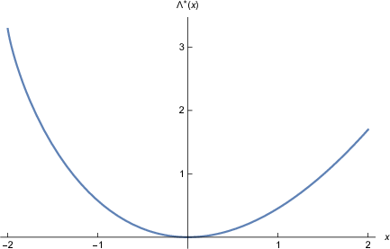
    (20) Λ∗​(x)={+∞x<−2,π23x=−2,h​(λ−1​(x),x)−2<x<0,h​(λ0​(x),x)x≥0,\Lambda^{*}\left(x\right)=\begin{cases}+\infty&x<-2,\\ \frac{\pi^{2}}{3}&x=-2,\\ h\left(\lambda_{-1}\left(x\right),x\right)&-2<x<0,\\ h\left(\lambda_{0}\left(x\right),x\right)&x\geq 0,\\ \end{cases}

    where

    h⁡(y,x)=y⁡(x+2)+2​Li⁡(1−ey),h\left(y,x\right)=y(x+2)+2\Li\left(1-e^{y}\right),
    λj​(x)=x+22+Wj​(−x+22​e−x+22),j∈{−1,0}.\lambda_{j}\left(x\right)=\frac{x+2}{2}+W_{j}\left(-\frac{x+2}{2}e^{-\frac{x+2}{2}}\right),\quad j\in\{-1,0\}.

    WjW_{j}, j∈{−1,0}j\in\{-1,0\} is the principal//lower branches of Lambert WW function respectively.

    Refer to caption
    Figure 1. The rate function Λ∗\Lambda^{*} for α=1\alpha=1

    Note that because Λ∗\Lambda^{*} is not symmetric the probability of the event |n1​(r)−μr|≥v1​(r)\left|n_{1}\left(r\right)-\mu_{r}\right|\geq v_{1}\left(r\right) is dominated by the event n1​(r)≥μr+t​v1​(r)n_{1}\left(r\right)\geq\mu_{r}+tv_{1}\left(r\right). Furthermore, the lower bound for the special case of the hole event when t=−2,α=1t=-2,\alpha=1 does not follow from the theory of large deviations, but can be computed directly (see [9, Section 5.1]).

  • •

    For α>1\alpha>1,

    (21) Λ∗​(x)={x24x≥0,+∞x<0.\Lambda^{*}\left(x\right)=\begin{cases}\frac{x^{2}}{4}&x\geq 0,\\ +\infty&x<0.\\ \end{cases}

A.3. Proof of Theorem 1.1

Next, assuming Lemma A.1, Theorem 1.1 follows from the Gartner-Ellis theorem:

Proof.

Notice that

ℙ[|∑k=1∞Xk−μr|≥t⋅v1(r)α]\displaystyle\mathbb{P}\left[\left|\sum_{k=1}^{\infty}X_{k}-\mu_{r}\right|\geq t\cdot v_{1}\left(r\right)^{\alpha}\right] =ℙ[|∑k=1∞(Xk−r2​k)|≥t⋅v1(r)α]\displaystyle=\mathbb{P}\left[\left|\sum_{k=1}^{\infty}\left(X_{k}-r^{2k}\right)\right|\geq t\cdot v_{1}\left(r\right)^{\alpha}\right]
=ℙ[|Zr|≥t]=ℙ[Zr∈(−∞,−t]∪[t,∞)]\displaystyle=\mathbb{P}\left[\left|Z_{r}\right|\geq t\right]=\mathbb{P}\left[Z_{r}\in\left(-\infty,-t\right]\cup\left[t,\infty\right)\right]
  • •

    For 12<α<1\frac{1}{2}<\alpha<1, it holds that

    infx∈(−∞,−t)∪(t,∞)​Λ∗​(x)=infx∈(−∞,−t]∪[t,∞)​12​x2=t22\underset{x\in\left(-\infty,-t\right)\cup\left(t,\infty\right)}{\inf}\Lambda^{*}\left(x\right)=\underset{x\in\left(-\infty,-t\right]\cup\left[t,\infty\right)}{\inf}\tfrac{1}{2}x^{2}=\frac{t^{2}}{2}

    thus,

    limr↑1ϵrlogμr((−∞,−t]∪[t,∞))=−t22,\underset{r\uparrow 1}{\lim}\epsilon_{r}\log\mu_{r}((-\infty,-t]\cup[t,\infty))=-\frac{t^{2}}{2},

    whence,

    −logℙ[|∑k=1∞Xk−μr|≥v1(r)α]∼t22v1(r)2​α−1,r↑1.-\log\mathbb{P}\left[\left|\sum_{k=1}^{\infty}X_{k}-\mu_{r}\right|\geq v_{1}\left(r\right)^{\alpha}\right]\sim{\frac{t^{2}}{2}v_{1}\left(r\right)^{2\alpha-1}},\quad r\uparrow 1.
  • •

    For α=1\alpha=1, it holds that

    infx∈(−∞,−t)∪(t,∞)​Λ∗​(x)=infx∈(−∞,−t]∪[t,∞)​Λ∗​(x)=min⁡{Λ∗​(−t),Λ∗​(t)}=Λ∗​(t)\underset{x\in\left(-\infty,-t\right)\cup\left(t,\infty\right)}{\inf}\Lambda^{*}\left(x\right)=\underset{x\in\left(-\infty,-t\right]\cup\left[t,\infty\right)}{\inf}\Lambda^{*}\left(x\right)=\min\left\{\Lambda^{*}\left(-t\right),\Lambda^{*}\left(t\right)\right\}=\Lambda^{*}\left(t\right)

    where the last equality also follows from Lemma A.2. Thus,

    limr↑1ϵrlogμr((−∞,−t]∪[t,∞))=−Λ∗(t)=−c(t),\underset{r\uparrow 1}{\lim}\epsilon_{r}\log\mu_{r}\left(\left(-\infty,-t\right]\cup\left[t,\infty\right)\right)=-\Lambda^{*}\left(t\right)=-c(t),

    whence,

    −logℙ[|∑k=1∞Xk−μr|≥t⋅v1(r)α]∼c⁡(t)4⋅(11−r)2​α−1,r↑1.-\log\mathbb{P}\left[\left|\sum_{k=1}^{\infty}X_{k}-\mu_{r}\right|\geq t\cdot v_{1}\left(r\right)^{\alpha}\right]\sim{\frac{c(t)}{4}\cdot\left(\frac{1}{1-r}\right)^{2\alpha-1}},\quad r\uparrow 1.
  • •

    For α>1\alpha>1, it holds that infx∈(−∞,−t)∪(t,∞)​14​x2=t24\underset{x\in\left(-\infty,-t\right)\cup\left(t,\infty\right)}{\inf}\tfrac{1}{4}x^{2}=\frac{t^{2}}{4} thus,

    limr↑1​ϵr​log⁡μr​([t,∞))=−t24,\underset{r\uparrow 1}{\lim}\epsilon_{r}\log\mu_{r}([t,\infty))=-\frac{t^{2}}{4},

    whence,

    −logℙ[|∑k=1∞Xk−μr|≥t⋅v1(r)α]∼t24v1(r)2​α−1,r↑1.-\log\mathbb{P}\left[\left|\sum_{k=1}^{\infty}X_{k}-\mu_{r}\right|\geq t\cdot v_{1}\left(r\right)^{\alpha}\right]\sim{\frac{t^{2}}{4}v_{1}\left(r\right)^{2\alpha-1}},\quad r\uparrow 1.

∎

Finally, we turn back to the calculation of the logarithmic moment generating function:

Proof of Lemma A.1.

Let λ∈ℝ\lambda\in\mathbb{R},

Λr​(ϵr−1​λ)\displaystyle\Lambda_{r}\left(\epsilon_{r}^{-1}\lambda\right) =Λr​(v1​(r)2​α−1​λ)=log⁡𝔼⁡[ev1​(r)2​α−1​λ​Zr]\displaystyle=\Lambda_{r}\left(v_{1}\left(r\right)^{2\alpha-1}\lambda\right)=\log\mathbb{E}\left[e^{v_{1}\left(r\right)^{2\alpha-1}\lambda Z_{r}}\right]
=log⁡𝔼⁡[ev1​(r)2​α−1​λ​1v1​(r)α​∑k=1∞(Xk−r2​k)]\displaystyle=\log\mathbb{E}\left[e^{v_{1}\left(r\right)^{2\alpha-1}\lambda\frac{1}{v_{1}\left(r\right)^{\alpha}}\sum_{k=1}^{\infty}\left(X_{k}-r^{2k}\right)}\right]
=log⁡𝔼⁡[ev1​(r)α−1​λ​∑k=1∞(Xk−r2​k)]=∑k=1∞log⁡𝔼⁡[ev1​(r)α−1​λ​(Xk−r2​k)]\displaystyle=\log\mathbb{E}\left[e^{v_{1}\left(r\right)^{\alpha-1}\lambda\sum_{k=1}^{\infty}\left(X_{k}-r^{2k}\right)}\right]=\sum_{k=1}^{\infty}\log\mathbb{E}\left[e^{v_{1}\left(r\right)^{\alpha-1}\lambda\left(X_{k}-r^{2k}\right)}\right]
=∑k=1∞log⁡(r2​k​ev1​(r)α−1​λ​(1−r2​k)+(1−r2​k)​ev1​(r)α−1​λ​(−r2​k))\displaystyle=\sum_{k=1}^{\infty}\log\left(r^{2k}e^{v_{1}\left(r\right)^{\alpha-1}\lambda\left(1-r^{2k}\right)}+\left(1-r^{2k}\right)e^{v_{1}\left(r\right)^{\alpha-1}\lambda\left(-r^{2k}\right)}\right)
=∑k=1∞log⁡(ev1​(r)α−1​λ​(−r2​k)​(r2​k​ev1​(r)α−1​λ+1−r2​k))\displaystyle=\sum_{k=1}^{\infty}\log\left(e^{v_{1}\left(r\right)^{\alpha-1}\lambda\left(-r^{2k}\right)}\left(r^{2k}e^{v_{1}\left(r\right)^{\alpha-1}\lambda}+1-r^{2k}\right)\right)
=∑k=1∞v1​(r)α−1​λ​(−r2​k)+∑k=1∞log⁡(1+r2​k​(ev1​(r)α−1​λ−1))\displaystyle=\sum_{k=1}^{\infty}v_{1}\left(r\right)^{\alpha-1}\lambda\left(-r^{2k}\right)+\sum_{k=1}^{\infty}\log\left(1+r^{2k}\left(e^{v_{1}\left(r\right)^{\alpha-1}\lambda}-1\right)\right)
=−μr​v1​(r)α−1​λ+∑k=1∞log⁡(1+r2​k​(ev1​(r)α−1​λ−1))=(⋆).\displaystyle=-\mu_{r}v_{1}\left(r\right)^{\alpha-1}\lambda+\sum_{k=1}^{\infty}\log\left(1+r^{2k}\left(e^{v_{1}\left(r\right)^{\alpha-1}\lambda}-1\right)\right)=(\star).

Put T:=ev1​(r)α−1​λ−1T:=e^{v_{1}\left(r\right)^{\alpha-1}\lambda}-1 and note that −1<T<+∞-1<T<+\infty , sgn​(T)=sgn​(λ)=sgn​(1+T​r2​k)\text{sgn}\left(T\right)=\text{sgn}\left(\lambda\right)=\text{sgn}\left(1+Tr^{2k}\right). We look at the map k→log⁡(1+T​r2​k)k\rightarrow\log\left(1+Tr^{2k}\right) on [0,∞)\left[0,\infty\right) and see that:

  • –

    For λ>0\lambda>0 the mapping decreases and its range is between log⁡(1+T)=v1​(r)α−1​λ\log\left(1+T\right)=v_{1}\left(r\right)^{\alpha-1}\lambda to 00.

  • –

    For λ<0\lambda<0 the mapping increases and its range is between v1​(r)α−1​λv_{1}\left(r\right)^{\alpha-1}\lambda to 00.

Hence, we can write

∑k=1∞log⁡(1+T​r2​k)=∫0∞log⁡(1+T​r2​x)​𝑑x+O⁡(v1​(r)α−1),\sum_{k=1}^{\infty}\log\left(1+Tr^{2k}\right)=\int_{0}^{\infty}\log\left(1+Tr^{2x}\right)dx+O\left(v_{1}\left(r\right)^{\alpha-1}\right),

and using the change of variables u=−T​r2​x,d​x=12​log⁡r​d​uuu=-Tr^{2x},\ dx=\frac{1}{2\log r}\frac{du}{u} we get

∑k=1∞log⁡(1+T​r2​k)\displaystyle\sum_{k=1}^{\infty}\log\left(1+Tr^{2k}\right) =−12​log⁡r∫0−Tlog⁡(1−u)udu+O(v1(r)α−1)\displaystyle=-\frac{1}{2\log r}\int_{0}^{-T}\frac{\log\left(1-u\right)}{u}du+O\left(v_{1}\left(r\right)^{\alpha-1}\right)
=12​log⁡r​Li2⁡(−T)+O⁡(v1​(r)α−1).\displaystyle=\frac{1}{2\log r}\Li_{2}\left(-T\right)+O\left(v_{1}\left(r\right)^{\alpha-1}\right).

Hence we get,

(⋆)=−μr​v1​(r)α−1​λ+12​log⁡r​Li2⁡(−T)+O⁡(v1​(r)α−1),(\star)=-\mu_{r}v_{1}\left(r\right)^{\alpha-1}\lambda+\frac{1}{2\log r}\Li_{2}\left(-T\right)+O\left(v_{1}\left(r\right)^{\alpha-1}\right),

therefore,

ϵr​Λr​(ϵr−1​λ)=−μr​v1​(r)−α​λ+v1​(r)−2​α+12​log⁡r​Li2⁡(−T)+o⁡(1).\epsilon_{r}\Lambda_{r}\left(\epsilon_{r}^{-1}\lambda\right)=-\mu_{r}v_{1}\left(r\right)^{-\alpha}\lambda+\frac{v_{1}\left(r\right)^{-2\alpha+1}}{2\log r}\Li_{2}\left(-T\right)+o(1).

Finally, all that’s left is to calculate

limr↑1(−μr​v1​(r)−α​λ+v1​(r)−2​α+12​log⁡r​Li2⁡(−T)).\lim_{r\uparrow 1}\left(-\mu_{r}v_{1}\left(r\right)^{-\alpha}\lambda+\frac{v_{1}\left(r\right)^{-2\alpha+1}}{2\log r}\Li_{2}\left(-T\right)\right).

We split the calculation into three cases based on the values of α\alpha and use the asymptotic properties of the Li2\text{Li}_{2} function that we noted in Section 1.2:

  1. (1)

    For 12<α<1\frac{1}{2}<\alpha<1, T→0T\rightarrow 0 when r↑1r\uparrow 1, hence T∼v1​(r)α−1​λT\sim v_{1}\left(r\right)^{\alpha-1}\lambda. Thus in this case

    Li2⁡(−T)∼v1​(r)α−1​λ+14​v1​(r)2​α−2​λ2,\Li_{2}\left(-T\right)\sim v_{1}\left(r\right)^{\alpha-1}\lambda+\frac{1}{4}v_{1}\left(r\right)^{2\alpha-2}\lambda^{2},

    therefore,

    −μr​v1​(r)−α​λ+v1​(r)−2​α+12​log⁡r​Li2⁡(−T)\displaystyle-\mu_{r}v_{1}\left(r\right)^{-\alpha}\lambda+\frac{v_{1}\left(r\right)^{-2\alpha+1}}{2\log r}\Li_{2}\left(-T\right)
    ∼−μr​v1​(r)−α​λ−v1​(r)−α2​log⁡r​λ−v1​(r)−2​α+12​log⁡r⋅v1​(r)2​α−2​λ24\displaystyle\sim-\mu_{r}v_{1}\left(r\right)^{-\alpha}\lambda-\frac{v_{1}\left(r\right)^{-\alpha}}{2\log r}\lambda-\frac{v_{1}\left(r\right)^{-2\alpha+1}}{2\log r}\cdot\frac{v_{1}\left(r\right)^{2\alpha-2}\lambda^{2}}{4}
    ∼−λ​v1​(r)−α​(μr+12​log⁡r)+λ22∼λ22,as​r↑1.\displaystyle\sim-\lambda v_{1}\left(r\right)^{-\alpha}\left(\mu_{r}+\frac{1}{2\log r}\right)+\frac{\lambda^{2}}{2}\sim\frac{\lambda^{2}}{2},\quad\text{as}\ r\uparrow 1.
  2. (2)

    For α=1\alpha=1 it follows immediately that Λ⁡(λ)=−2​λ−2​Li2⁡(1−eλ)\Lambda\left(\lambda\right)=-2\lambda-2\Li_{2}\left(1-e^{\lambda}\right).

  3. (3)

    For α>1\alpha>1,

    • •

      If λ<0\lambda<0, T→−1T\rightarrow-1 when r↑1r\uparrow 1, hence Li2⁡(−T)→Li2⁡(1)=π26\Li_{2}\left(-T\right)\rightarrow\Li_{2}\left(1\right)=\frac{\pi^{2}}{6}. Thus

      limr↑1−μrv1(r)−αλ+v1​(r)−2​α+12​log⁡rLi2(−T)=limr↑1−2v1(r)1−α−2v1(r)2−2​απ26=0.\lim_{r\uparrow 1}-\mu_{r}v_{1}\left(r\right)^{-\alpha}\lambda+\frac{v_{1}\left(r\right)^{-2\alpha+1}}{2\log r}\Li_{2}\left(-T\right)=\lim_{r\uparrow 1}-2v_{1}\left(r\right)^{1-\alpha}-2v_{1}\left(r\right)^{2-2\alpha}\frac{\pi^{2}}{6}=0.
    • •

      If λ>0\lambda>0, T→+∞T\rightarrow+\infty when r↑1r\uparrow 1 hence T∼ev1​(r)α−1T\sim e^{v_{1}\left(r\right)^{\alpha-1}}. So in this case

      Li2⁡(z)∼−12​log2⁡(T)∼−12​v1​(r)2​α−2​λ2,\Li_{2}\left(z\right)\sim-\frac{1}{2}\log^{2}\left(T\right)\sim-\frac{1}{2}v_{1}\left(r\right)^{2\alpha-2}\lambda^{2},

      thus

      limr↑1−μrv1(r)−αλ+v1​(r)−2​α+12​log⁡rLi2(−T)\displaystyle\lim_{r\uparrow 1}-\mu_{r}v_{1}\left(r\right)^{-\alpha}\lambda+\frac{v_{1}\left(r\right)^{-2\alpha+1}}{2\log r}\Li_{2}\left(-T\right)
      =limr↑1−2v1(r)1−αλ−(2v1(r)2−2​α)(−12v1(r)2​α−2λ2)=λ2.\displaystyle=\lim_{r\uparrow 1}-2v_{1}\left(r\right)^{1-\alpha}\lambda-\left(2v_{1}\left(r\right)^{2-2\alpha}\right)\left(-\frac{1}{2}v_{1}\left(r\right)^{2\alpha-2}\lambda^{2}\right)=\lambda^{2}.
    • •

      For λ=0\lambda=0, ϵr​Λr​(ϵr−1​λ)=0\epsilon_{r}\Lambda_{r}\left(\epsilon_{r}^{-1}\lambda\right)=0,

proving the claim. ∎

During the proof we used the formula for Λ∗\Lambda^{*} in the case α=1\alpha=1, we calculate it as follows:

Lemma A.2.
Λ∗​(x)={+∞x<−2,π23x=−2,h​(λ−1​(x),x)−2<x<0,h​(λ0​(x),x)x≥0,\Lambda^{*}\left(x\right)=\begin{cases}+\infty&x<-2,\\ \frac{\pi^{2}}{3}&x=-2,\\ h\left(\lambda_{-1}\left(x\right),x\right)&-2<x<0,\\ h\left(\lambda_{0}\left(x\right),x\right)&x\geq 0,\\ \end{cases}

where

h⁡(y,x)=y⁡(x+2)+2​Li⁡(1−ey),h\left(y,x\right)=y(x+2)+2\Li\left(1-e^{y}\right),
λj​(x)=x+22+Wj​(−x+22​e−x+22),j∈{−1,0}.\lambda_{j}\left(x\right)=\frac{x+2}{2}+W_{j}\left(-\frac{x+2}{2}e^{-\frac{x+2}{2}}\right),\quad j\in\{-1,0\}.

WjW_{j}, j∈{−1,0}j\in\{-1,0\} is the principal//lower branches of Lambert WW function respectively.

Proof.

Define h⁡(λ)=λ⁡(x+2)+2​Li2⁡(1−eλ).h\left(\lambda\right)=\lambda\left(x+2\right)+2\Li_{2}\left(1-e^{\lambda}\right). It holds that

limλ→+∞h⁡(λ)=limλ→+∞λ⁡(x+2)−π23−log2⁡(eλ−1)=−∞,\lim_{\lambda\rightarrow+\infty}h\left(\lambda\right)=\lim_{\lambda\rightarrow+\infty}\lambda\left(x+2\right)-\frac{\pi^{2}}{3}-\log^{2}\left(e^{\lambda}-1\right)=-\infty,
limλ→−∞h⁡(λ)=limλ→−∞λ⁡(x+2)+2​Li2⁡(1)={2​Li2​(1)=π23x=−2,+∞x<−2,−∞x>−2.\lim_{\lambda\rightarrow-\infty}h\left(\lambda\right)=\lim_{\lambda\rightarrow-\infty}\lambda\left(x+2\right)+2\Li_{2}\left(1\right)=\begin{cases}2\Li_{2}\left(1\right)=\frac{\pi^{2}}{3}&x=-2,\\ +\infty&x<-2,\\ -\infty&x>-2.\\ \end{cases}

Consider the equation,

(22) y​ey=−12​(x+2)​e−12​(x+2),y=λ−12​(x+2).ye^{y}=-\frac{1}{2}{\left(x+2\right)}e^{-\tfrac{1}{2}{\left(x+2\right)}},y=\lambda-\frac{1}{2}{\left(x+2\right)}.

Hence,

y=W⁡(−12​(x+2)​e−12​(x+2))⟹λ=12​(x+2)+W⁡(−12​(x+2)​e−12​(x+2)).y=W\left(-\frac{1}{2}\left(x+2\right)e^{-\tfrac{1}{2}{\left(x+2\right)}}\right)\implies\lambda=\frac{1}{2}\left(x+2\right)+W\left(-\frac{1}{2}{\left(x+2\right)}e^{-\tfrac{1}{2}{\left(x+2\right)}}\right).

W0​(0)=0,W0​(−1e)=−1W_{0}\left(0\right)=0,W_{0}\left(-\frac{1}{e}\right)=-1 and W−1W_{-1} decreases from W−1​(−1e)=−1W_{-1}(-\frac{1}{e})=-1 to W−1​(0−)=−∞W_{-1}\left(0^{-}\right)=-\infty. Furthermore, it holds that:

limx→∞W0​(x)log⁡(x)=1,limx→0−W−1​(x)log⁡(−x)=1.\lim_{x\rightarrow\infty}\frac{W_{0}\left(x\right)}{\log\left(x\right)}=1\ ,\ \lim_{x\rightarrow 0^{-}}\frac{W_{-1}\left(x\right)}{\log\left(-x\right)}=1.

Observe that since h′h^{\prime} is monotone decreasing, when −2<x<0-2<x<0, λ\lambda has to be negative hence by (A.3) and the fact that 12​(x+2)≤1\frac{1}{2}{\left(x+2\right)}\leq 1, WW has to be less than −1-1 so in this case we’ll choose the branch W−1W_{-1}. By the same argument when x≥0x\geq 0 we’ll choose W0W_{0}. Let us denote the solution according to the branches λ0/−1(x)\lambda_{0/-1}(x) and overall we get-

Λ∗​(x)={+∞x<−2,π23x=−2,h​(λ−1​(x),x)−2<x<0,h​(λ0​(x),x)x≥0.\Lambda^{*}\left(x\right)=\begin{cases}+\infty&x<-2,\\ \frac{\pi^{2}}{3}&x=-2,\\ h\left(\lambda_{-1}\left(x\right),x\right)&-2<x<0,\\ h\left(\lambda_{0}\left(x\right),x\right)&x\geq 0.\\ \end{cases}

It holds that

limx↓−2Λ∗​(x)=limx↓−2(x+2)​(12​(x+2)+W−1​(−12​(x+2)​e−12​(x+2)))\displaystyle\lim_{x\downarrow-2}\Lambda^{*}\left(x\right)=\lim_{x\downarrow-2}\ \left(x+2\right)\left(\frac{1}{2}\left(x+2\right)+W_{-1}\left(-\frac{1}{2}\left(x+2\right)e^{-\frac{1}{2}{\left(x+2\right)}}\right)\right)
+2​Li2⁡(1−exp⁡(12​(x+2)+W−1​(−12​(x+2)​e−12​(x+2))))\displaystyle+2\Li_{2}\left(1-\exp\left(\frac{1}{2}\left(x+2\right)+W_{-1}\left(-\frac{1}{2}\left(x+2\right)e^{-\frac{1}{2}\left(x+2\right)}\right)\right)\right) =π23,\displaystyle=\frac{\pi^{2}}{3},

and

limx→+∞Λ∗​(x)=limx→+∞(x+2)​(12​(x+2)+W0​(−12​(x+2)​e−12​(x+2)))\displaystyle\lim_{x\rightarrow+\infty}\Lambda^{*}\left(x\right)=\lim_{x\rightarrow+\infty}\ \left(x+2\right)\left(\frac{1}{2}{\left(x+2\right)}+W_{0}\left(-\frac{1}{2}{\left(x+2\right)}e^{-\tfrac{1}{2}{\left(x+2\right)}}\right)\right)
+2​Li2⁡(1−exp⁡(12​(x+2)+W0​(−12​(x+2)​e−12​(x+2))))\displaystyle+2\Li_{2}\left(1-\exp\left({\frac{1}{2}{\left(x+2\right)}+W_{0}\left(-\frac{1}{2}{\left(x+2\right)}e^{-\frac{1}{2}{\left(x+2\right)}}\right)}\right)\right) =+∞,\displaystyle=+\infty,

where the asymptotic of the functions W0,W−1,Li2W_{0},W_{-1},\Li_{2} is used for both limits. Note that Λ∗​(0)=0\Lambda^{*}\left(0\right)=0 and that the function Λ∗\Lambda^{*} is non-negative in a neighborhood of 00 hence by convexity, 00 is the minimum of this function (see Figure 1), completing the proof of Lemma A.2 and of Theorem 1.1.

∎

Appendix B Measurability of β∗\beta^{*}

Recall that β∗:Ω→[0,2​π)\beta^{*}:\Omega\rightarrow[0,2\pi) is such that

1N​∑j=1Nlog⁡|f⁡(r0​ei​θj⋅ei​β∗)|=∫r0​𝕋log⁡|f|​𝑑μ\frac{1}{N}\sum_{j=1}^{N}\log\left|f\left(r_{0}e^{i\theta_{j}}\cdot e^{i\beta^{*}}\right)\right|=\int_{r_{0}\mathbb{T}}\log\left|f\right|d\mu

when f≠0f\neq 0 otherwise we set β∗=0\beta^{*}=0. We understand our probability space Ω\Omega as follows. Consider the complex plane ℂ\mathbb{C} with ℂν\mathbb{C}_{\nu} the Borel sigma-algebra of ℂ\mathbb{C}. Then, we take the countable product measure space ℂν∞\mathbb{C}^{\infty}_{\nu}, with the sigma algebra generated by cylinder sets, i.e. ℂj−1×Uj×ℂn−j\mathbb{C}^{j-1}\times U_{j}\times\mathbb{C}^{n-j} where Uj∈ℬ⁡(ℂ)U_{j}\in\mathcal{B}\left(\mathbb{C}\right), n≥1n\geq 1. Denote by A​(𝔻)\text{A}\left(\mathbb{D}\right) - the space of analytic functions defined on the unit disk. Endow this space with the topology of uniform convergence on compact sets. This makes it a complete separable metric space. Now, β∗:Ω↦[0,2​π)\beta^{*}:\Omega\mapsto[0,2\pi) can be viewed as a composition of two measurable functions. The map ω={ωn}n=1∞↦f⁡(z,ω)=∑n=1∞ξn​(ω)​zn\omega=\{\omega_{n}\}_{n=1}^{\infty}\mapsto f\left(z,\omega\right)=\sum_{n=1}^{\infty}\xi_{n}\left(\omega\right)z^{n} where ξn​(ω)=ωn\xi_{n}\left(\omega\right)=\omega_{n} is measurable as a limit of measurable functions (projections are continuous). Then, we need to prove that the map β∗:A⁡(𝔻)↦[0,2​π]\beta^{*}:A\left(\mathbb{D}\right)\mapsto[0,2\pi] defined momentarily is measurable.

Consider all β\beta’s such that

1N​∑j=1Nlog⁡|f⁡(r0​ei​θj⋅ei​β)|=∫r0​𝕋log⁡|f|​𝑑μ=:cf\frac{1}{N}\sum_{j=1}^{N}\log\left|f\left(r_{0}e^{i\theta_{j}}\cdot e^{i\beta}\right)\right|=\int_{r_{0}\mathbb{T}}\log\left|f\right|d\mu=:c_{f}

(such β\beta exists as we’ve already mentioned by continuity, Equation 8). We define β∗​(f):A​(𝔻)→[0,2​π]\beta^{*}\left(f\right):\text{A}\left(\mathbb{D}\right)\rightarrow\left[0,2\pi\right] as follows:

β∗​(f)=inf{β∈[0,2​π):1N​∑j=1Nlog⁡|f⁡(r0​ei​θj⋅ei​β)|=cf}.\beta^{*}\left(f\right)=\inf\{\beta\in[0,2\pi)\ :\ \frac{1}{N}\sum_{j=1}^{N}\log\left|f\left(r_{0}e^{i\theta_{j}}\cdot e^{i\beta}\right)\right|=c_{f}\}.

To see that β∗\beta^{*} is lower semi-continuous (and hence measurable), we want to show that for all a∈[0,2​π)a\in[0,2\pi), {f∈A​(𝔻):β∗​(f)>a}∈ℬA​(r​𝔻¯)\{f\in\text{A}\left(\mathbb{D}\right)\ :\ \beta^{*}\left(f\right)>a\}\in\mathcal{B}_{\text{A}\left(r\bar{\mathbb{D}}\right)} where ℬA​(r​𝔻¯)\mathcal{B}_{\text{A}\left(r\bar{\mathbb{D}}\right)} is the Borel sigma-algebra with respect to the sup metric. (since r<1r<1 is fixed, we can restrict our domain to r​𝔻r\mathbb{D}.) Indeed,

{f∈A\displaystyle\{f\in\text{A} (𝔻):β∗(f)>a}\displaystyle\left(\mathbb{D}\right)\ :\ \beta^{*}\left(f\right)>a\}
={f∈A(𝔻):∀β∈[0,a],1N∑j=1Nlog|f(r0ei​θj⋅ei​β)|≠cf}\displaystyle=\bigg\{f\in\text{A}\left(\mathbb{D}\right)\ :\ \forall\beta\in\left[0,a\right]\ ,\ \frac{1}{N}\sum_{j=1}^{N}\log\left|f\left(r_{0}e^{i\theta_{j}}\cdot e^{i\beta}\right)\right|\neq c_{f}\bigg\}
=⋃n{f∈A(𝔻):∀β∈[0,a],|1N∑j=1Nlog|f(r0ei​θj⋅ei​β)|−cf|>1n}\displaystyle=\bigcup_{n}\,\bigg\{f\in\text{A}\left(\mathbb{D}\right)\ :\ \forall\beta\in\left[0,a\right]\ ,\ \Big|\frac{1}{N}\sum_{j=1}^{N}\log\big|f\left(r_{0}e^{i\theta_{j}}\cdot e^{i\beta}\right)\big|-c_{f}\Big|>\frac{1}{n}\bigg\}

So if supr​𝔻¯|f−g|<δ\sup_{r\bar{\mathbb{D}}}\left|f-g\right|<\delta then (by continuity) the integrals are sufficiently close to each other |cf−cg|<ϵ\left|c_{f}-c_{g}\right|<\epsilon hence this set is open.

References

  • [1] J. Buckley, Fluctuations in the zero set of the hyperbolic Gaussian analytic function. Int. Math. Res. Not. IMRN 6, (2015).
  • [2] J. Buckley and A. Nishry, Precise deviations for disk counting statistics of invariant determinantal processes. arXiv:2104.12598 (2021)
  • [3] J. Buckley, A. Nishry, R. Peled, and M. Sodin, , Hole probability for zeroes of Gaussian Taylor series with finite radii of convergence. Probab. Theory Related Fields 171, (2018).
  • [4] R. M. Corless, G. H. Gonnet, D. E. G. Hare, D. J. Jeffrey, and D. E .Knuth, On the Lambert WW function. Adv. Comput. Math. 5, (1996).
  • [5] A. Dembo and O. Zeitouni, Large deviations techniques and applications. Springer-Verlag, Berlin, 2010.
  • [6] M. Fenzl and G. Lambert, Precise deviations for disk counting statistics of invariant determinantal processes. arXiv:2003.07776 (2020)
  • [7] P. J. Forrester and G. Honner, Exact statistical properties of the zeros of complex random polynomials. J. Phys. A 32, (1999).
  • [8] S. Ghosh and A. Nishry, Gaussian complex zeros on the hole event: the emergence of a forbidden region. Comm. Pure Appl. Math. 72, (2019).
  • [9] J. Hough, M. Krishnapur, Y. Peres, and B. Virág, Zeros of Gaussian analytic functions and determinantal point processes. American Mathematical Society, Providence, RI, 2009.
  • [10] A. Kiro and A. Nishry, Fluctuations for zeros of Gaussian Taylor series. Journal of the London Mathematical Society , (2021).
  • [11] M. Krishnapur, Overcrowding estimates for zeroes of planar and hyperbolic Gaussian analytic functions. J. Stat. Phys. 124, (2006).
  • [12] L. Lewin, Polylogarithms and associated functions. North-Holland Publishing Co., New York-Amsterdam, (1981).
  • [13] F. Nazarov and M. Sodin, Fluctuations in random complex zeroes: asymptotic normality revisited. Int. Math. Res. Not. IMRN 24, (2011).
  • [14] F. Nazarov, M. Sodin, and A. Volberg, The Jancovici-Lebowitz-Manificat law for large fluctuations of random complex zeroes. Comm. Math. Phys. 284, (2008).
  • [15] A. Nishry, Asymptotics of the hole probability for zeros of random entire functions. Int. Math. Res. Not. IMRN 15, (2010).
  • [16] A. Nishry, Hole probability for entire functions represented by Gaussian Taylor series. J. Anal. Math. 118, (2012).
  • [17] Y. Peres and B. Virág, Zeros of the i.i.d. Gaussian power series: a conformally invariant determinantal process. Acta Math. Related Fields 194, (2005).
  • [18] M. Sodin, Zeros of Gaussian analytic functions. Math. Res. Lett. 7, (2000).
  • [19] M. Sodin and B. Tsirelson, Random complex zeroes. III. Decay of the hole probability. Israel J. Math. 147, (2005).
  • [20] M. Sodin and B. Tsirelson, Random complex zeroes. I. Asymptotic normality. Israel J. Math. 144, (2004).