Quasi-optimal -finite element refinements towards singularities via deep neural network prediction
Abstract
We show how to construct the deep neural network (DNN) expert to predict quasi-optimal -refinements for a given computational problem. The main idea is to train the DNN expert during executing the self-adaptive -finite element method (-FEM) algorithm and use it later to predict further refinements. For the training, we use a two-grid paradigm self-adaptive -FEM algorithm. It employs the fine mesh to provide the optimal refinements for coarse mesh elements. We aim to construct the DNN expert to identify quasi-optimal refinements of the coarse mesh elements. During the training phase, we use the direct solver to obtain the solution for the fine mesh to guide the optimal refinements over the coarse mesh element. After training, we turn off the self-adaptive -FEM algorithm and continue with quasi-optimal refinements as proposed by the DNN expert trained. We test our method on three-dimensional Fichera and two-dimensional L-shaped domain problems. We verify the convergence of the numerical accuracy with respect to the mesh size. We show that the exponential convergence delivered by the self-adaptive -FEM can be preserved if we continue refinements with a properly trained DNN expert. Thus, in this paper, we show that from the self-adaptive -FEM it is possible to train the DNN expert the location of the singularities, and continue with the selection of the quasi-optimal refinements, preserving the exponential convergence of the method.
Keywords:
-adaptive finite element , deep neural networks , direct solvers1 Introduction
The application of the neural networks in adaptive finite element method usually supports the generation of the adaptive mesh [36] or mesh partitioning algorithms [35]. In this paper, we focus on adaptive finite element method. It can approximate a given problem with prescribed accuracy using a minimal number of basis functions. It employs a mesh to approximate a given problem using a linear combination of basis functions spanning the computational mesh. It improves approximation quality by generating new basis functions for a better approximation. The new basis functions are obtained by breaking selected elements into smaller elements and spanning smaller basis functions there (this process is called refinement). We may also obtain them by adding new higher-order basis functions over existing elements (this process is called the refinement). The refinement is the combination of both. It has been proven theoretically and experimentally [18, 19, 21], that the adaptive algorithm can deliver the best possible exponential convergence of the numerical error with respect to the mesh size.
There are several implementations of the data structures supporting -refinements [11, 12, 27, 6, 33, 9]. In this paper, we focus on the data structure proposed by Demkowicz [12, 27], supporting hanging nodes and the 1-irregularity rule. This code also contains the implementation of the fully automatic self-adaptive finite element method algorithm (self-adaptive -FEM), described in [26, 27]. It employs the two-grid paradigm. It compares numerical solutions on the two grids, the actual (the coarse) and the reference (the fine) grid. Each finite element from the coarse mesh, it considers different refinement strategies. For each strategy, it computes the error decrease rate. It estimates how much error decrease we gain by selecting this local element refinement, divided by how many degrees of freedom we have to invest to get there. For evaluating the error decrease rate, it employs the projections from the fine mesh local element solution into the considered refinement strategy of the coarse mesh element. This strategy selects the optimal refinements for particular elements. It delivers the exponential convergence, which has been verified experimentally for a large class of problems [11, 12].
However, this implementation of the self-adaptive -FEM algorithm is expensive. It requires the solutions to the computational problem over the coarse and fine mesh in several iterations. In particular, the fine mesh problem is usually one order of magnitude larger than the actual coarse mesh problem in two dimensions and two orders of magnitude larger in 3D. The computational grids are highly non-uniform; they contain elongated elements and different polynomial orders of approximations. Thus, the iterative solvers deliver convergence problems [23, 30, 22], and the computationally expensive [8, 25] direct solvers [14, 15] augmented with proper ordering algorithms [31, 2, 17] are employed to solve the coarse and the fine mesh problems. Additionally, selecting the optimal refinements involves computations of local projections and multiple possibilities to consider over the coarse mesh elements.
Here we propose an artificial expert, Deep Neural Network (DNN), selecting refinements for particular elements of the computational mesh. The DNN expert focus on the key problem in the implementation of the self-adaptive -FEM, namely the selection of the optimal refinements for the mesh elements. We train the DNN expert during the execution of the self-adaptive -FEM algorithm. We collect the dataset for all the decisions made by the self-adaptive -FEM. The input to the DNN is element data, such as its location, sizes, and actual polynomial orders of approximations. The output from the DNN is the decision about optimal refinements. We train the DNN to make quasi-optimal decisions about optimal refinements. When the DNN is ready to make quasi-optimal decisions, we turn off the computationally intense self-adaptive -FEM, and we ask the DNN-driven -FEM to predict the optimal refinements. Our DNN-based expert can learn the locations of the singularities where the refinements are needed, as well as the patterns for performing the refinements.
The DNN has already been applied for -adaptive finite element method in two-dimensions [24]. The experiments presented there concern the case of the DNN training to learn the optimal -refinements for a given class of boundary-value problems to apply the trained DNN for new problems from the same class. Our paper differs from [24] in three aspects. First, we generalize the DNN-driven -FEM algorithm into three dimensions. Second, we train the DNN expert to propose further quasi-optimal refinements for a given computational problem when the self-adaptive algorithm runs out of resources or becomes computationally too intense. Third, in [24], the DNN is trained to make decisions about local element refinement by using the input data, including the local solution. We can only use the DNN from [24] after we call a solver. This makes it impossible to use that DNN to guide further refinements without calling the solver. In this paper, we train the DNN for the two- and 3D problem, using as input the element coordinates and the actual polynomial orders of approximation over the element. In this way, our DNN-based expert learns the locations of singularities, the geometric patterns for refinements, and the patterns for modification of the polynomial orders of approximation. Thus, we propose a DNN expert that allows continuing with refinements beyond the reach of the solver.
The DNN-based expert training methodology proposed in this paper can guide refinements in different computational codes, including the codes developed by the group of Leszek Demkowicz [11, 12], or the codes using a hierarchy of nested meshed for performing the refinements [10, 33, 9, 28, 29]. The generalization of the idea presented in this paper to different basis functions and multiple hanging nodes requires modification of the input and/or output of the DNN. The DNN, once trained, proposes quasi-optimal refinements for finite elements from the actual computational mesh.
The structure of the paper is the following. Section 2 is the Preliminaries where we introduce our model problem, some basic definitions and the self-adaptive -FEM algorithm. Section 3 introduces the architecture of the neural network and the DNN-driven -FEM algorithm. Section 4 presents the numerical results for the model L-shape domain problem and the model Fichera problem defined as the superposition of several model L-shaped domain problems. We conclude the paper in Section 5.
2 Preliminaries
2.1 Model problem and variational formulations
Let , with , be a bounded, open and simply connected polyhedron, and denote by its boundary assumed to be split into two disjoint open and not empty subsets . That is, and . Using the standard notations for Hilbert spaces, for a given source term , we look for an approximation of the solution satisfying:
| (1) |
Introducing the Hilbert space , problem (1) admits the following well-posed continuous variational formulation [12]:
| (2) |
The discrete formulation
| (3) |
The discrete space is constructed with hierarchical basis functions obtained by glueing together the element shape functions. The shape functions are constructed as tensor products of 1D hierarchical-shape functions
2.2 Self-adaptive finite element method
In this Section, we briefly discuss the self-adaptive -FEM algorithm, following the ideas described by Demkowicz et al. [11, 12]. We, however, propose a slightly different algorithm, with the differences explained inside this Section.
The self-adaptive -FEM algorithm is based on a two-grid paradigm. A computation over a coarse mesh, and a computation over a fine mesh.
Definition 1.
The initial coarse mesh is obtained by partitioning the domain into a finite set of hp finite elements and selecting arbitrary polynomial orders of approximation.
Definition 2.
Coarse mesh problem: Find coefficients (dofs) of approximate solution fulfilling (6).
Definition 3.
The coarse mesh approximation space is defined as
where is a global basis function (element basis of ), is a shape function and is the mapping over the coarse mesh assigning global number of dofs (basis functions) related with shape function from element
Remark 1.
The approximation space with basis is constructed by gluing together element-local-shape functions.
Definition 4.
The fine mesh is obtained by breaking each element from the coarse mesh into 8 elements (in 3D) and increasing the polynomial orders of approximation by one.
Definition 5.
Fine mesh problem: Find coefficients (dofs) of approximate solution fulfilling (6).
Definition 6.
The fine mesh approximation space is defined as
where is a basis function (element basis of ), is a shape function, is the mapping over the fine mesh assigning global number of dofs (basis function) related to shape function from element .


: 

2 Solve the coarse mesh problem using direct solver to obtain
3 Generate fine mesh by breaking each element of the coarse mesh into 8 elements and increasing polynomial orders by 1
4 Solve the fine mesh problem using direct solver to obtain
5 Compute
6 if maximum relative error accuracy then
8 Perform all hp refinements from to obtain
9 (coarse mesh = optimal mesh)
10 goto 2
Having the self-adaptive -FEM algorithm defined in Algorithm 1, we focus on Algorithm 2, selecting the optimal refinement for a given coarse mesh element.
Our Algorithm 2, however, differs from the one described by Demkowicz [12] in the following aspect. We select optimal refinements for interiors of finite elements (see Figure 2 for the two-dimensional case), and we adjust the faces and edges accordingly. In the original algorithm described in [12], the optimal refinements are first selected for finite element edges, then for faces, and finally for the interiors. The recursive structure of the original algorithm as proposed by [12] enables reduction of the computational cost since the selection of the optimal refinements for edges restricts the number of possibilities for refinements of faces, see Figure 3. Similarly, the selection of optimal refinements for faces restricts the number of possible refinements for the interiors.
Our motivation to replace this original three-step algorithm proposed by Demkowicz [12] by the one-step Algorithm 2 is the following. We plan to replace the Algorithm 2 by DNN. Once trained, the DNN can provide the quasi-optimal refinement for the interior of the element in a linear computational cost (very fast).

(this simplified picture does not include different orders on edges)

(this simplified picture does not include different orders on edges)
In the one-step Algorithm 2, the selection of the optimal refinements is performed by computing the error decrease rate for all considered refinement strategies. The is defined as the gain in the reduction of the approximation error divided by the loss defined as the number of degrees of freedom added. The reduction of the approximation error is estimated as , where denotes the relative error of the coarse mesh element solution with respect to the fine mesh solution computed in norm over the element , and denotes the relative error of the solution corresponding to the proposed refinement strategy with respect to the the fine mesh solution . The difference is the error decrease (how much the error go down if we switch from into be performing the proposed refinement of the coarse mesh element solution. For each considered refinement strategy, the solution corresponding to the refined coarse mesh element is obtained by the projection from the fine mesh solution . The procedure is called projection-based interpolation, and it is described in [13].
for approximation space do
Compute the error decrease rate
if then
Select corresponding to as the optimal refinement for element end if
Select orders on edges = MIN (orders from neighboring faces)
The fine mesh elements are employed to localize the 8 elements corresponding to given coarse mesh element , and to compute the projections of the fine mesh solution into the interpolant .
The following definition formally explains that the optimal refinement for a given element is the refinement that provides the maximum error decrease rate.
Definition 7.
Let be the coarse and fine mesh approximation spaces. Let represents the coarse mesh elements.
and are coarse / fine mesh problem solutions.
The approximation space is called the optimal approximation space over an element , if the projection based interpolant of into over element realizes the following maximum
where is the projection-based interpolant of into over element , and
Note that the selection of the optimal refinement in the Algorithm 2 is based on the coarse and fine mesh solutions. We plan to train the DNN to select quasi-optimal refinements based on the location of elements and actual polynomial orders of approximation, to continue with the refinement once the solver runs out of resources.
3 Deep neural network-driven -adaptive finite element method algorithm
We propose the following architecture of the DNN that learns the quasi-optimal refinements.


We use a feed-forward DNN with fully connected layers [7], presented in Figures 4-5 The network splits into five branches in 2D and nine branches in 3D, four layers each: the first branch decides about the optimal refinement, and the remaining branches decide about modifying the polynomial orders - refinement. Since all possible decisions are encoded as categorical variables, we use cross-entropy as the loss function.
Each layer learns a certain transformation and applies a non-linear activation function – in this case, the ReLU function [1]. To prevent overfitting, we use the DropOut mechanism [32], which randomly samples a subset of neurons in each layer and sets their activation to 0 during the training phase. This increases the network’s potential to generalize. The last layer uses linear activation, which is well suited for regression tasks.
As the output vector dimensionality is distinctly greater than the input data, and additionally highly structural (-adaptation, the orders for eight elements polynomial interpolators), the respective NN cannot have a simple dense MLP architecture. For example, the predicted values of output vector coordinates may be mutually exclusive. In that case, the volume of the space of irrational solutions is huge and can overwhelm that representing rational ones. Consequently, the NN aproximator will be overfitted, producing mainly useless solutions. Splitting the hidden layers of NN on separate paths, each controlling only those output neurons which represent the same type of information (h-adaptation, element 1 polynomial order, element 2 polynomial order, …, element 8 polynomial order), limits considerably the volume of solution and parameter spaces. Thus, concentrating the approximator on rational solutions. In the extreme case (all hidden layers are split), we train simultaneously several MLPs on the same data but concentrated on various goals (outputs). Adding more initial not split hidden layers with a considerably larger number of neurons than the input layer allows for finding a better representation of input data.
Now we are ready to introduce DNN-driven -FEM Algorithm 3 that guides the refinements. It does not employ the two-grid paradigm; its decisions about quasi-optimal refinements result from asking the trained DNN.
2 (coarse mesh = initial mesh)
3 Solve the coarse mesh problem to obtain (optional)
4 if iterations # iterations then
6 Perform all hp refinements from to obtain
7 (coarse mesh = optimal mesh)
8 ++#iterations
9 goto 2
Note that the call to the solver in Line 3 is optional, it is only intended to provide the energy norm estimation of the solution in order to monitor the convergence.
4 Numerical results


In this section, we present two numerical experiments.
The first experiment concerns the DNN-driven -FEM for the two-dimensional L-shaped domain model problem with fixed boundary conditions. The first numerical experiment’s goal is to verify the convergence of the DNN-driven -FEM algorithm as compared to the self-adaptive -FEM algorithm
The second experiment concerns the DNN-driven -FEM for the 3D Fichera model problem. The second numerical experiment aims to verify if we can train the DNN using the geometrical data from 12 iterations of the self-adaptive -FEM to learn the locations of singularities and the distribution patterns of the polynomial orders of approximation.
4.1 Verification of the method using two-dimensional L-shaped domain problem
As the first problem, we consider the diffusion problem (3) defined in the L-shaped domain . We set and as the Dirichlet and Neumann boundaries, respectively (see Figure 6(a)). As source term, we consider such that the analytical solution of Problem (3) coincides with , explicitly defined in polar coordinates as:
| (4) |
The gradient of the analytical solution is singular at point and belongs to the Hilbert space , for all (see [34]). Last implies in practice that, to resolve the singularity with high accuracy, several -refinements and non-uniform distribution of polynomial orders of approximations are required in the layers surrounding the entrant corner (cf. [18, 19].)
We run the self-adaptive -FEM algorithm in the model L-shaped domain problem. We collect the decisions about the optimal refinements for the coarse mesh elements. We run 40 iterations of the self-adaptive -FEM algorithm, and we collect the data summarized in Tables 1-2 as the dataset for training. We collect around 10,000 samples for the dataset by recording the decisions about the optimal refinements performed for particular finite elements.
Having the DNN trained, we continue with the L-shaped domain problem computations. We run 10 iterations of the DNN-driven -FEM. In this 2D problem, we can also continue with the self-adaptive -FEM algorithm (running without the DNN). Thus, we compare last 10 iterations of our DNN-driven -FEM against the last 10 iterations of the self-adaptive -FEM algorithm.
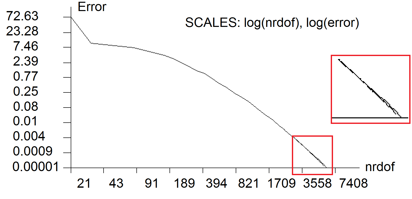
We compare the exponential convergence of the self-adaptive -FEM and the DNN-driven -FEM algorithms in Figure 7. We can see that both methods deliver similar exponential convergence, and we have trained the DNN very well. We compare in Figures 8-11 the final mesh generated by both methods. The last 10 iterations of the DNN-driven -FEM algorithm performs refinements similar to the last 10 iterations of the self-adaptive -FEM. The difference concerns very small elements, with a diameter of , depicted in Figure 11. We conclude that in two dimensions, we can effectively train the DNN, so it predicts the optimal refinements and delivers exponential convergence.
| Input parameter | Data dimensionality |
|---|---|
| Element coordinates | 4 |
| double precision | |
| Element dimensions | 2 |
| double precision | |
| polynomial order of approximation for element | 2 |
| where | integer |
| Output parameter | Data dimensionality |
|---|---|
| refinement flag | 3 |
| , where | boolean |
| polynomial order of approximation for element 1 | 2 |
| where | integer |
| polynomial order of approximation for element 2 | 2 |
| where | integer |
| polynomial order of approximation for element 3 | 2 |
| where | integer |
| polynomial order of approximation for element 4 | 2 |
| where | integer |


and by 40 iterations of self-adaptive -FEM followed by 10 iterations of the deep learning-driven -FEM algorithm (right panel).


and by 40 iterations of self-adaptive -FEM followed by 10 iterations of the deep learning-driven -FEM algorithm (right panel). Zoom 100 X


and by 40 iterations of self-adaptive -FEM followed by 10 iterations of the deep learning-driven -FEM algorithm (right panel). Zoom 10,000 X


and by 40 iterations of self-adaptive -FEM followed by 10 iterations of the deep learning-driven -FEM algorithm (right panel).
Zoom 1,000,000 X
4.2 Three-dimensional Fichera model problem
This 3D problem was introduced by Gaetano Fichera [16] as the benchmark to test the convergence of 3D finite element method codes. It has a point singularity in the central point (0,0,0) and three edge-singularities around the three central edges.
This problem is the generalization of the L-shaped domain model problem into three dimensions. We seek the temperature scalar field over . We set and as the Dirichlet and Neumann boundaries, respectively (see Figure 6(b)). The Neumann boundary condition is obtained from the superposition of three solutions of the two-dimensional L-shaped domain model problem. The details of the formulation are provided in [26].
| (5) |
We consider the weak formulation
| (6) |
and introduce proper Sobolev space
| (7) |
To resolve the one point and three edge singularities with high accuracy, this problem requires several refinements towards the edges and non-uniform distribution of polynomial orders of approximations in the layers surrounding the central point and the three edges.
In this numerical experiment, we run Algorithms 1 and 2 of the self-adaptive -FEM algorithm for 12 iterations of the Fichera model problem. Figure 12 presents the sequence of generated meshes. We collect around 2000 samples for the dataset. The input and the output employed for the training of the DNN are summarized in Tables 3-4. The DNN learns the location of the singularities, where the refinements are needed, based on the geometrical coordinates and dimensions of the finite elements. It also learns the refinement patterns, using the geometrical data and the element distribution of the polynomial approximation orders.
| Input parameter | Data dimensionality |
|---|---|
| Element coordinates | 6 |
| double precision | |
| Element dimensions | 3 |
| double precision | |
| Polynomial orders of approximation for element interior | 3 |
| integer |
| Output parameter | Data dimensionality |
|---|---|
| refinement flag | 3 |
| , where | boolean |
| polynomial order of approximation for element 1 | 2 |
| where | integer |
| polynomial order of approximation for element 2 | 2 |
| where | integer |
| polynomial order of approximation for element 3 | 2 |
| where | integer |
| polynomial order of approximation for element 4 | 2 |
| where | integer |
| polynomial order of approximation for element 5 | 2 |
| where | integer |
| polynomial order of approximation for element 6 | 2 |
| where | integer |
| polynomial order of approximation for element 7 | 2 |
| where | integer |
| polynomial order of approximation for element 8 | 2 |
| where | integer |


The Algorithm 1 of the self-adaptive -FEM algorithm employs the two grids paradigm. It solves the problem over the coarse and the fine mesh, using the MUMPS solver [3, 4, 5]. In this 3D model problem, the memory requirements and the execution times for the coarse and fine mesh problems are summarized in Figures 13-14.


We stop the self-adaptive -FEM algorithm after 12 iterations. We use the collected 2000 samples to train the DNN. This time no calling the solver, we continue the refinements by using Algorithm 3 of the DNN-driven -FEM. The further sequence of meshes generated by the DNN-driven -FEM algorithm is presented in Figure 15.
In order to verify the convergence of the DNN-driven -FEM, we estimate the energy norm of the solution on the sequence of coarse grids generated by either self-adaptive -FEM or DNN-driven -FEM, and the fine grids for the case of th self-adaptive -FEM. The convergence plots are summarized in Figure 16. By using the energy norm of the finest solution obtained on the fine mesh from twelve iterations of the self-adaptive -FEM algorithm, we can plot the convergence of the relative error of the self-adaptive -FEM and the DNN-driven -FEM, presented in Figure 17. The red line denotes the moment when we finish the self-adaptive -FEM (e.g., the fine mesh solver runs out of resources), and we continue with the DNN-driven -FEM. As a result, we obtain a very nice exponential convergence. To understand these results, we must remember that we compute the relative error with respect to the energy norm of the finest mesh solution.


4.3 Deep Neural Network Training
We train the network for 200 epochs using the Adam optimizer [20], which minimizes the Mean Squared Error cost function. The error backpropagation algorithm uses information from the optimizer to correct the network’s weights. We can modify the magnitude of that correction by changing the learning rate constant. In addition, we regularize the network by reducing the learning rate whenever the loss function minimization slows down. We also use early stopping to stop the training procedure before completing all 200 training epochs if the difference in results between epochs is insignificant and cannot be improved by the learning rate reduction scheme. We used the TensorFlow 1.13 and CUDA 9 library to train the network on an nVidia Tesla v100 GPU with 32GB VRAM and 64GB general-purpose RAM.
Figure 18 illustrates the training procedure in 3D. The dataset is partitioned into 80% of training and 20% validation sets. During each epoch, we train the DNN using the training dataset. After each training epoch, the DNN is tested against the validation subset. The plots in Figure 18 denote the percentage of the correctly predicted refinements and refinements taking into account all validation datasets. Accuracy equal to 1.0 means the DNN makes 100 percent of incorrect decisions concerning the refinements.
The training in the 3D case is based on the 1132 samples generated during the execution of the twelve iterations of the self-adaptive -FEM algorithm on the Fichera model problem. The DNN has learned well the locations of the singularities, so it can propose optimal refinements along the three edges of the Fichera corner. The DNN has also learned how to distribute the polynomial orders of approximation. As we can read from the numerical results section, this enabled to continue with the exponential convergence.
Figure 19 illustrates the training procedure in two dimensions. The dataset partitioning and the training procedure are similar to those in 3D. The plots in Figure 19 denote the percentage of the correctly predicted refinements and refinements considering all validation datasets. Accuracy of refinement equal to 0.97 means the DNN makes 97 percent of correct decisions concerning the refinements. Accuracy equal to 0.95 means the DNN makes 5 percent of incorrect decisions concerning the refinements.
The training in the 2D case is based on the 10,000 samples generated during the 40 iterations of the self-adaptive -FEM algorithm on the L-shaped domain model problem. In this case, learning how to refine means learning the location of the point singularity at point (0,0). The DNN has learned the locations of this point singularity well so that it can propose the optimal refinements there. The DNN has also learned well the distribution of the polynomial orders of approximation from the 10,000 samples, with around 95 percent of correct decisions. As discussed in the numerical results section, this enabled us to maintain exponential convergence.


5 Conclusions
We showed that an artificial expert can learn the optimal refinement patterns for a given computational problem. We proposed the Deep Neural Network driven -FEM algorithm (Algorithm 3), guiding the quasi-optimal refinements for the finite element method. The algorithm can be trained using the self-adaptive -FEM for a given problem. The self-adaptive -FEM uses an expensive direct solver to guide the optimal refinements. When we run out of resources, we can turn off the self-adaptive -FEM, collect the decisions about the optimal refinements, and train the DNN. We can continue later with quasi-optimal refinements as guided by the DNN-driven -FEM. Instead of calling an expensive solver, we can ask the DNN expert to propose the refinements. Our method has been verified 2D and 3D dimensions using the model L-shaped domain and the Fichera problems. In particular, we showed that we could obtain a high-quality DNN expert by using only element locations and refinement patterns.
Acknowledgments
The European Union’s Horizon 2020 Research and Innovation Program of the Marie Skłodowska-Curie grant agreement No. 777778, MATHROCKs. Research project partly supported by program "Excellence initiative – research university" for the University of Science and Technology.
References
- [1] A. F. Agarap, Deep learning using rectified linear units (ReLu). arXiv preprint arXiv:1803.08375 (2018).
- [2] P. R. Amestoy, T. A. Davis, I. S. Du, An Approximate Minimum Degree Ordering Algorithm, SIAM Journal of Matrix Analysis & Application, 17, 4 (1996) 886-905.
- [3] P. R. Amestoy and I. S. Duff, Multifrontal parallel distributed symmetric and unsymmetric solvers, Computer Methods in Applied Mechanics and Engineering, 184 (2000) 501-520.
- [4] P. R. Amestoy, I. S. Duff, J. Koster and J-Y L’Excellent, A fully asynchronous multifrontal solver using distributed dynamic scheduling, SIAM Journal on Matrix Analysis and Applications, 1(23) (2001) 15-41.
- [5] P. R. Amestoy, A. Guermouche, J-Y L’Excellent and S. Pralet, Hybrid scheduling for the parallel solution of linear systems, Computer Methods in Applied Mechanics and Engineering 2(32) (2001), 136–156.
- [6] R. E. Bank, A. H. Sherman, A. Weiser, Some refinement algorithms and data structures for regular local mesh refinement, Scientific Computing, Applications of Mathematics and Computing to the Physical Sciences 1 (1983) 3–17.
- [7] G. Bebis, M. Georgiopoulos, Feed-forward neural networks, IEEE Potentials 13(4) (1994) 27-31.
- [8] V. M. Calo, N. Collier, D. Pardo, M. Paszyński, Computational complexity and memory usage for multi-frontal direct solvers used in p finite element analysis, Procedia Computer Science 4 (2011) 1854-1861.
- [9] D. D’Angella, N. Zander, S. Kollmannsberger, F. Frischmann, E. Rank, A. Schrǒder, A. Reali, Multi-level -adaptivity and explicit error estimation, Advanced Modeling and Simulation in Engineering Sciences, 3(33) (2016)
- [10] V. Darrigrand, D. Pardo, T. Chaumont-Frelet, I. Gómez-Revuelto, L. E. Garcia-Castillo, A painless automatic hp-adaptive strategy for elliptic problems, Finite Elements in Analysis and Design, 178 (2020) 103424
- [11] L. Demkowicz, (2006). Computing with hp-Adaptive Finite Elements, Vol. I. Two Dimensional Elliptic and Maxwell Problems. Chapman and Hall/Crc Applied Mathematics and Nonlinear Science.
- [12] Demkowicz, L., Kurtz, J., Pardo, D., Paszyński, M., Rachowicz, W., & Zdunek, A. (2007). Computing with hp-Adaptive Finite Elements, Vol. II. Frontiers. Three Dimensional Elliptic and Maxwell Problems with Applications. Chapman and Hall/Crc Applied Mathematics and Nonlinear Science.
- [13] L. Demkowicz, A. Buffa, , and -conforming projection-based interpolation in three dimensions: Quasi-optimal p-interpolation estimates, Computer Methods in Applied Mechanics and Engineering 194(2-5) (2005) 267-296.
- [14] I. S. Duff, J. K., Reid The multifrontal solution of indefinite sparse symmetric linear systems. ACM Transactions on Mathematical Software, 9 (1983) 302-325.
- [15] I. S. Duff, J. K. Reid, The multifrontal solution of unsymmetric sets of linear systems., SIAM Journal on Scientific and Statistical Computing, 5 (1984) 633-641.
- [16] G. Fichera, Numerical and quantitative analysis, Surveys and Reference Works in Mathematics, vol. 3, London–San Francisco–Melbourne: Pitman Publishing, (1978)
- [17] G.W. Flake, R.E. Tarjan, K. Tsioutsiouliklis, Graph clustering and minimum cut trees, Internet Mathematics 1 (2003), 385-408.
- [18] B. Guo, I. Babuška, The version of the finite element method, Part I: The basic approximation results, Computational Mechanics, 1(1) (1986) 21-41.
- [19] B. Guo, I. Babuška, The version of the finite element method, Part II: General results and applications, Computational Mechanics, 1(1) (1986) 203-220.
- [20] D. P. Kingma, J. Ba. Adam: A method for stochastic optimization. arXiv preprint arXiv:1412.6980 (2014)
- [21] W. F. Mitchell, M. A. McClain, A comparison of hp-adaptive strategies for elliptic partial differential equations, ACM Transactions on Mathematical Software (TOMS) 41(1), 2 (2014)
- [22] D. Pardo, J. Álvarez-Aramberri, M. Paszyński, L. Dalcin, V. M. Calo, Impact of element-level static condensation on iterative solver performance, Computers & Mathematics with Applications 70 (10), (2015) 2331-2341.
- [23] D. Pardo, L. Demkowicz, Integration of hp-adaptivity and a two-grid solver for elliptic problems, Computer Methods in Applied Mechanics and Engineering 195(7) (2006) 674-710
- [24] M. Paszyński, R. Grzeszczuk, D. Pardo, L. Demkowicz, Deep learning driven self-adaptive finite element method, Lecture Notes in Computer Science (2021)
- [25] M. Paszyński, V. M. Calo, D. Pardo, Direct solvers performance on h-adapted grids Computers & Mathematics with Applications 70 (3) (2015) 282-295.
- [26] W. Rachowicz, D. Pardo, L. Demkowicz, Fully automatic hp-adaptivity in three dimensions, Computer Methods in Applied Mechanics and Engineering 195(37-40) (2006) 4816-4842
- [27] W. Rachowicz, J. T. Oden, L. Demkowicz, Toward a universal adaptive finite element strategy, Part 3. Design of meshes, Computer Methods in Applied Mechanics and Engineering, 77, 181–212 (1989)
- [28] E. Rank Adaptive remeshing and domain decomposition, Computer Methods in Applied Mechanics and Engineering, 101(1) (1992) 299–313.
- [29] E. Rank, R. Krause, A multiscale finite-element-method. Computers & Structures 64 (1995) 139–44.
- [30] Y. Saad, Iterative Methods for Sparse Linear Systems, Society for Industrial and Applied Mathematics; 2nd edition (2003)
- [31] J. Schulze, Towards a tighter coupling of bottom-up and top-down sparse matrix ordering methods, BIT, 41, 4 (2001) 800.
- [32] N. Srivastava, et al. Dropout: a simple way to prevent neural networks from overfitting, The journal of machine learning research 15(1) (2014) 1929-1958.
- [33] N. Zander, T. Bog, S. Kollmannsberger, E. Rank, The multi-level -method for three-dimensional problems: dynamically changing high-order mesh refinement with arbitrary hanging nodes, Computer Methods in Applied Mechanics and Engineering, 310 (2016) 252-277.
- [34] M.-C Rivara, Mesh refinement processes based on the generalized bisection of simplices, SIAM J. Numer. Anal., 21 (3) (1984), 604-613.
- [35] A. Bahreininejad, B. H. V. Topping, A. I. Khan, Finite element mesh partitioning using neural networks. Advances in Engineering Software, 27(1-2) (1996) 103-115.
- [36] M. N. Jadid, D. R. Fairbairn, The application of neural network techniques to structural analysis by implementing an adaptive finite-element mesh generation. AI EDAM, 8(3) (1994) 177-191.