Phase Dependent Loss Analysis for RIS Systems

Research into reconfigurable intelligent surfaces (RISs) has shown that intelligently tuning the RIS phases can significantly improve performance in wireless systems. However, such works usually assume that reflections from the RIS elements experience a constant attenuation. This is an over-simplification and assumes that the power of the reflected signal is independent of the phase shift at each RIS element. In this paper, we focus on the more general case [1], where the RIS phases affect the reflected signal strength, i.e., phase dependent loss (PDL). As an initial investigation, we focus on the effects of PDL on single user (SU) systems.

For SU systems, [2] derives a closed form expression for the mean SNR where the user (UE) to RIS and RIS to base station (BS) channels experience Rayleigh fading and the direct channel between UE and BS is absent. [3] derives an exact expression for the optimal uplink (UL) mean SNR for systems where the UE-BS channel is rank-1 LOS and the UE-RIS and UE-BS channels are correlated Rayleigh. The LOS assumption in the RIS-BS channel has been considered and motivated in numerous works (e.g [4]). The authors in [3] leverage the mean SNR expression to provide insight on the impact of correlation on the mean SNR. In [5], the authors extend the exact mean SNR derivation in [3] to systems where the UE-BS and UE-RIS channels are correlated Ricean and derive a tight approximation to the mean rate. The authors again, leverage the mean SNR expression to provide insight on the impact of correlation and the Rician K-factor on the mean SNR. However, the analysis in [2, 3, 5] assumes either perfect RIS reflection or reflections with constant attenuation.

In [1], a mathematical model is proposed for PDL. Numerical results in [1] show that the model accurately matches the reflective response of a detailed circuit model for a semiconductor device used to construct typical RIS elements. Furthermore, characteristics of the circuit model resemble experimental results in the literature [1].

To best of our knowledge, no analysis is available to characterise optimal system performance with PDL. Hence, the contributions of this paper are as follows:

• •

  An exact mean SNR expression is derived for the optimal RIS phases using the PDL model in [1]. The optimal RIS design is based on the lossless case as there is no known optimal design in the presence of PDL. A simple rule of thumb is also provided to evaluate the effects of PDL.

• •

  We analytically characterise the impact of the parameters in the loss function (attenuation function) on the mean SNR. The loss function is defined by three parameters; $L_{\mathrm{min}}$: the minimum amplitude of the loss function; $\alpha$: the steepness of the loss function; $\theta$: the shift of the loss function. These parameters are dependent on the circuit used to construct typical semiconductors for RIS reflective elements.

• •

  Numerical results validate the derived SNR expression and verify the impact of the loss function parameters $L_{\mathrm{min}},\alpha,\theta$ on the mean SNR. We show that any impact caused by the loss function on the mean SNR becomes more pronounced as the size of the RIS increases. For typical parameter values, these effects are significant.

Notation: $\mathbb{E}\left\{\cdot\right\}$ represents statistical expectation. $\Re\left\{\cdot\right\}$ is the Real operator. $\left\lVert\cdot\right\rVert_{2}$ denotes the $\ell_{2}$ norm. Upper and lower boldface letters represent matrices and vectors, respectively. $\mathcal{CN}(\bm{\mu},\mathbf{Q})$ denotes a complex Gaussian distribution with mean $\bm{\mu}$ and covariance matrix $\mathbf{Q}$. $\mathcal{U}[a,b]$ denotes a uniform distribution on $[a,b]$. The transpose, Hermitian transpose and complex conjugate operators are denoted as $(\cdot)^{T},(\cdot)^{H},(\cdot)^{*}$, respectively. The trace and diagonal operators are denoted by $\mathrm{tr}\left\{\mathbf{\cdot}_{\mathrm{}}\right\}$ and $\text{diag}\{\cdot\}$, respectively. The angle of a vector $\mathbf{x}_{\mathrm{}}$ of length $N$ is defined as $\angle\mathbf{x}_{\mathrm{}}=[\angle x_{1},\ldots,\angle x_{N}]^{T}$ along with $\left\lvert\mathbf{x}\right\rvert=[\left\lvert x_{1}\right\rvert,\ldots,\left\lvert x_{N}\right\rvert]^{T}$. The exponential of a vector is defined as $e^{\mathbf{x}_{\mathrm{}}}=[e^{x_{1}},\ldots,e^{x_{N}}]^{T}$. $\otimes$ denotes the Kronecker product. $\mathrm{B}\left(z,w\right)$ denotes the beta function with parameters $z,w$. $\mathbf{1}_{N}$ denotes an $N\times 1$ vector with unit entries.

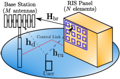
As shown in Fig. 1, we examine a RIS-aided single input multiple output (SIMO) system where a RIS with $N$ reflective elements is located close to a BS with $M$ antennas such that a rank-1 LOS condition is achieved between the RIS and BS.

Here, we provide an exact result for the mean SNR, $\mathbb{E}\left\{\mathrm{SNR}\right\}$, building on the results in [3] for the mean SNR in a lossless scenario.

Note that $F$ is the only variable dependent on the correlations in $\mathbf{h}_{\mathrm{ru}}$ and also note that the variable $L_{rs}$ is a double integral of the loss function. In Sec. III-A and Sec. III-B, we derive exact results for special cases of $F$, $L_{rs}$ when $\left\lvert\rho_{rs}\right\rvert\in\{0,1\}$. These correlation extremes provide useful benchmarks to evaluate the SNR trends.

In this section, we explore the impact of the circuit-dependent parameters $L_{\mathrm{min}},\alpha,\theta$ on the mean SNR. These parameters only impact the variables $\mu_{1},\mu_{2},L_{rs}$ in the mean SNR expression (7). While the broad impact of $L_{\mathrm{min}},\alpha,\theta$ is intuitive from the loss function (2), in this section we present analysis to support and quantify these effects.

We present numerical results to verify the analysis in Sec. IV. Firstly, note that we do not consider cell-wide averaging as the focus is on the SNR distribution over the fast fading. Hence, we present numerical results for fixed link gains for which the geometric model for the deployment of the UE, BS and RIS is adopted from [8] and shown in Fig. 2.

In particular, since the RIS-BS link is LOS, we assume $\beta_{\mathrm{br}}=d_{\mathrm{br}}^{-2}$ where $d_{\mathrm{br}}=51$m. For the other channels, we use the distance-dependent path loss model,

where $C_{0}=-30$ dB is the path loss at a reference distance of 1m, $d_{\mathrm{ru}}=21.0238$m and $d_{\mathrm{d}}=30.167$m is the UE-RIS and UE-BS separation distances respectively, $\alpha_{\mathrm{ru}}=2.8$ and $\alpha_{\mathrm{d}}=3.5$ are the path loss exponents for the UE-RIS and UE-BS channels respectively. These values give the path gains of $\beta_{\mathrm{d}}=-81.7077$ dB and $\beta_{\mathrm{ru}}=-67.0360$ dB. Distances $d_{\mathrm{ru}}$ and $d_{\mathrm{d}}$ were computed using elementary trigonometry where $d=30$m and $d_{\mathrm{v}}=1$m. The power of the transmitted signal is $E_{s}=1$ and the noise power is $\sigma^{2}=-65$ dBm.

As stated in Sec. II-A, the steering vectors for $\mathbf{H}_{\mathrm{br}}$ are not restricted to any particular structure. However, for simulation purposes, we will use the VURA model as outlined in [9], but in the $y-z$ plane with equal spacing in both dimensions at both the RIS and BS. The $y$ and $z$ components of the steering vector at the BS are $\mathbf{a}_{\mathrm{b,y}}$ and $\mathbf{a}_{\mathrm{b,z}}$ which are given by

respectively. Similarly at the RIS, $\mathbf{a}_{\mathrm{r,y}}$ and $\mathbf{a}_{\mathrm{r,z}}$ are defined by,

respectively, where $M=M_{y}M_{z}$, $N=N_{y}N_{z}$ with $M_{y},M_{z}$ being the number of antenna columns and rows at the BS and $N_{y},N_{z}$ being the number of columns and rows of RIS elements. $d_{\mathrm{b}}=0.5$ and $d_{\mathrm{r}}$ are BS/RIS element spacings in wavelength units. Note that the value of $d_{\mathrm{r}}$ is set to satisfy a particular correlation level $\mathrm{sinc}(2d_{\mathrm{r}})=\rho_{\mathrm{ru}}$ as per (4). The steering vectors at the BS and RIS are then given by,

respectively. $\theta_{\mathrm{A}}$ and $\omega_{\mathrm{A}}$ are elevation/azimuth angles of arrival (AOAs) at the BS and $\theta_{\mathrm{D}},\omega_{\mathrm{D}}$ are the corresponding angles of departure (AODs) at the RIS. The elevation/azimuth angles are selected based on the following geometry representing a range of LOS $\mathbf{H}_{\mathrm{br}}$ links with less elevation variation than azimuth variation: $\theta_{D}\sim\mathcal{U}[70^{o},90^{o}],\hskip 10.00002pt\omega_{D}\sim\mathcal{U}[-30^{o},30^{o}],\hskip 10.00002pt\theta_{A}=180^{o}-\theta_{D},\hskip 10.00002pt\omega_{A}\sim\mathcal{U}[-30^{o},30^{o}]$. For all results in this paper we use a single sample from this range of angles given by $\theta_{D}=77.1^{o},\omega_{D}=19.95^{o},\theta_{A}=109.9^{o},\omega_{A}=-29.9^{o}$.

In Fig. 3, we verify the mean SNR expression in (7) for varying values of $N$ and $L_{\mathrm{min}}=0.5,\alpha=1.2,\theta=0.2,\rho_{\mathrm{d}}=0.7,\rho_{\mathrm{ru}}\in\{0,0.95,1\}$. For the special cases of $\rho_{\mathrm{ru}}=0$ and $\rho_{\mathrm{ru}}=1$, we use the expressions (15) and (17) to compute the variable $F$, respectively. For all correlation and RIS size scenarios, the analytical mean SNR agrees with simulations. Notice that even with PDL, the mean SNR grows as $\mathcal{O}(N^{2})$, identical to the growth of the mean SNR without PDL [10]. Also shown is the trivial approximation where every element, $L(\phi_{n})$, of the loss matrix is replaced by the mean of the loss function, $\mu_{1}$. As can be seen, this simple amplitude scaling gives a reasonable lower bound and is a useful rule of thumb.

In Fig. 4, we compute the analytical and simulated mean SNR for varying values of $\alpha$, and $L_{\mathrm{min}}\in\{0.1,0.5,0.95\},N\in\{16,64\},\theta\in\{0.2,0.42\},\rho_{\mathrm{d}}=\rho_{\mathrm{ru}}=0.7$.

It is observed in Fig. 4 that the mean SNR monotonically decreases in $\alpha$ which agrees with the analysis in Sec. IV. Increasing the value of $L_{\mathrm{min}}$ increases the mean SNR which also agrees with the analysis. Furthermore, notice that as $L_{\mathrm{min}}\to 1$, the mean SNR becomes nearly constant for all values of $\alpha$ which agrees with analysis in that no loss is observed at $L_{\mathrm{min}}=1$. As $\alpha\to 0$, the mean SNR converges to the same value for all $L_{\mathrm{min}}$ scenarios as per the analysis. Furthermore, notice that for both $N=16$ and $N=64$ scenarios, the mean SNR curves are identical for both $\theta=0.2$ and $\theta=0.42$. Hence, offsetting the loss function (2) by $\theta$ does not affect the mean SNR as shown in the analysis

Next, we further examine how $\alpha$ and $L_{\mathrm{min}}$ affect the mean SNR by considering different RIS sizes. In Fig. 4, the initial drop off in mean SNR is steeper for the $N=64$ scenario compared to the scenario where $N=16$. Hence, as the number of RIS elements increases, the initial drop off in mean SNR is more pronounced. Also notice in Fig. 4 that when $N=16$, the separation gap between the mean SNR curves for the three $L_{\mathrm{min}}$ values is smaller than those in the case of $N=64$. Therefore, as the number of RIS elements increases, altering $L_{\mathrm{min}}$ has a greater effect on the mean SNR. Typical parameter values $L_{\mathrm{min}}=0.2,\alpha=1.6$ are given in [1]. From Fig. 4, we see that the drop in SNR for these parameters and $N=64$ is bracketed by the $\alpha\in\{0.1,0.5\}$ curves and is between 48% and 74%. Hence we can expect a significant reduction in mean SNR for practical RIS systems.

We derive an exact closed form expression for the mean SNR where the RIS elements experience PDL. Specifically, the amplitude of the reflections from the RIS element are dependent on the optimal RIS phases which maximize the SNR in the absence of PDL. The attenuation function used for PDL was developed from a detailed circuit analysis of RIS elements, and is dependent on three parameters which control the minimum amplitude, steepness and shift of the attenuation function. We analytically characterise the impact of PDL on the mean SNR, offering insight into how PDL impacts the mean SNR performance. The analysis shows that the mean SNR only depends on the minimum amplitude and the steepness parameters. Having a larger minimum amplitude increases the mean SNR and having a steeper attenuation function decreases the mean SNR. This effect is enhanced when the number of RIS elements increases.

References

• [1] S. Abeywickrama et al., “Intelligent reflecting surface: Practical phase shift model and beamforming optimization,” IEEE Trans. Commun., vol. 68, no. 9, pp. 5849–5863, 2020.
• [2] A.-A. A. Boulogeorgos and A. Alexiou, “Performance analysis of reconfigurable intelligent surface-assisted wireless systems and comparison with relaying,” IEEE Access, vol. 8, pp. 94 463–94 483, 2020.
• [3] I. Singh et al., “Optimal SNR analysis for single-user RIS systems,” in Proc. IEEE PIMRC, 2021, pp. 1–6.
• [4] Q. Nadeem et al., “Asymptotic max-min SINR analysis of reconfigurable intelligent surface assisted MISO systems,” IEEE Trans. Wireless Commun., pp. 1–1, 2020.
• [5] I. Singh et al., “Optimal SNR analysis for single-user RIS systems in Ricean and Rayleigh environments,” IEEE Trans. Wireless Commun., pp. 1–1, 2022.
• [6] E. Björnson and L. Sanguinetti, “Rayleigh fading modeling and channel hardening for reconfigurable intelligent surfaces,” IEEE Wireless Commun. Lett., vol. 10, no. 4, pp. 830–834, 2021.
• [7] I. S. Gradshteyn and I. M. Ryzhik, Table of Integrals, Series, and Products. Elsevier Inc., 2007.
• [8] Q. Wu and R. Zhang, “Intelligent reflecting surface enhanced wireless network via joint active and passive beamforming,” IEEE Trans. Wireless Commun., vol. 18, no. 11, pp. 5394–5409, 2019.
• [9] C. L. Miller et al., “Analytical framework for full-dimensional massive MIMO with ray-based channels,” IEEE J. Sel. Topics Signal Process., vol. 13, no. 5, pp. 1181–1195, 2019.
• [10] I. Singh et al., “Optimal SNR analysis for single-user RIS systems,” in Proc. IEEE PIMRC, 2021, pp. 549–554.
• [11] S. Li et al., “Analysis of analog and digital MRC for distributed and centralized MU-MIMO systems,” IEEE Trans. Veh. Technol., vol. 68, no. 2, pp. 1948–1952, 2019.
• [12] K. S. Miller, Complex Stochastic Processes: An Introduction to Theory and Application. Addison-Wesley Publishing Company, Advanced Book Program, 1974.
• [13] B.-N. Guo and F. Qi, “Sharpening and generalizations of Carlson’s inequality for the arc cosine function,” arXiv preprint arXiv:0902.3495, 02 2009.
• [14] M. Abramowitz and I. A. Stegun, Handbook of Mathematical Functions with Formulas, Graphs, and Mathematical Tables. Dover, 1964.