Joint Constraints on Exoplanetary Orbits from Gaia DR3 and Doppler Data
Abstract
The third Gaia data release includes a catalog of exoplanets and exoplanet candidates identified via the star’s astrometric motion. This paper reports on tests for consistency between the Gaia two-body orbital solutions and precise Doppler velocities, for the stars currently amenable to such a comparison. For BD-17 0063, HD 81040, and HD 132406, the Gaia orbital solution and the Doppler data were found to be consistent, and were fitted jointly to obtain the best possible constraints on the planets’ orbits and masses. Inconsistencies were found for 4 stars: HD 111232, probably due to additional planets that were not included in the astrometric model; HD 175167 and HR 810, possibly due to inaccurate treatment of non-Gaussian uncertainties in the Gaia orbital solutions; and HIP 66074, for unknown reasons. Consistency tests were also performed for HD 114762, which was reported in 1989 to have a brown dwarf or exoplanet but has since been shown to be binary star. The joint Gaia-Doppler analysis shows the secondary mass to be and the orbital inclination to be degrees.
I Introduction
The astrometric technique for exoplanet detection is based on sensing a star’s reflex motion projected onto the sky plane. It is the oldest method for generating exoplanet candidates (Strand 1943, see, e.g.,), and has recently come back to prominence thanks to data from the Gaia Collaboration et al. 2022a. As part of Data Release 3 (DR3), Holl et al. 2022 presented a catalog of candidate exoplanets that includes 73 astrometric detections.
The astrometric method for planet detection is important because it can reveal all of a planet’s orbital parameters and uniquely specify its mass (Quirrenbach 2010, see, e.g.,). However, despite the unprecedented precision of Gaia astrometry, the current data are only sensitive to giant planets, and even then, the signal-to-noise ratios are typically modest (10). With current Doppler spectrographs, giant planets can be detected with much higher signal-to-noise ratios, but the Doppler data do not reveal the orbital inclination and give only a lower limit on the planet’s mass. Thus, the two techniques are complementary.
The Gaia Collaboration et al. 2022b highlighted 11 astrometrically detected exoplanets for which high-precision Doppler data are already available, and compared the published Doppler-based values of the orbital period and eccentricity with the values determined by Gaia. The good matches served to validate the methods that were used to derive orbital parameters from the Gaia astrometry, although the team also noted some discrepancies. In keeping with the desire for the initial DR3 publications to be based solely on Gaia data insofar as possible, the Gaia team did not perform joint fitting of the astrometric and Doppler data. Doing so would allow for a more thorough evaluation of the consistency between the two datasets, and would also provide the best possible constraints on the planets’ masses and orbital parameters. That was the purpose of the work described in this paper.
While analyzing the planet-hosting stars, the opportunity was also taken to revisit HD 114762 b, the erstwhile exoplanet candidate discovered by Latham et al. 1989. Astrometric data from Gaia has already shown that the orbit is viewed nearly face-on and that the companion’s mass exceeds the minimum mass of a star (Kiefer 2019; Holl et al. 2022), but the results of joint Gaia-Doppler fitting have not yet been reported.
II Sample Selection
A straightforward approach to determining the orbital parameters would be to fit a two-body model to the combination of radial-velocity and astrometric time-series data. However, the Gaia time-series astrometric data have not yet been released. Instead, DR3 provides a summary of the results of fitting a two-body model to the astrometric time-series data. This information is sufficient for present purposes, but only when the star’s radial-velocity variations and astrometric motion are both dominated by the effect of a single planet. When multiple planets make detectable contributions to the star’s motion, the results of a two-body fit are difficult to interpret, at best, and meaningless, at worst. Therefore, the list of stars to be analyzed was restricted to those for which which useful Doppler data are available and only a single giant planet has been reported.
This narrowed down the list to 7 stars (in addition to the special case of HD 114762, described above). For one of those stars, HIP 66074, the Gaia astrometry triggered the initial detection of the planet, although a small amount of precise radial-velocity data had previously been obtained as part of a Doppler survey. For the other 6 stars, BD-17 0063, HD 81040, HD 132406, HD 111232, HR 810, and HD 175167, the planet was initially discovered via the Doppler method. The stars that needed to be rejected on account of having multiple known companions were HD 142 (Wittenmyer et al. 2012), HD 164604 (Arriagada et al. 2010), and GJ 876 (Marcy et al. 2001). Another star, HIP 28193, was excluded because the available radial-velocity data are sparse and affected by stellar activity (Holl et al. 2022).
Table 1 gives a summary of the Doppler data gathered from the literature. The results of the two-body fits to the Gaia data were obtained from the gaiadr3.nss_two_body_orbits table at the Gaia archive.11 1 https://gea.esac.esa.int/archive/ The gaiadr3.astrophysical_parameters table (Creevey et al. 2022) was also consulted to obtain the stellar properties determined by the General Stellar Parametrizer from Spectroscopy (gspspec) and Photometry (gspphot), as well as the stellar mass from the Final Luminosity Age Mass Estimator (FLAME).
| Star | Instrument | # of | Median | Timespan | Time range | Reference |
|---|---|---|---|---|---|---|
| name | name | RVs | unc. (m/s) | (days) | (year/month) | |
| BD-17 0063 | HARPS | 26 | 1.5 | 1760 | 2003/10–2008/08 | Moutou et al. 2009 |
| HD 81040 | ELODIE | 23 | 12 | 1210 | 2002/02–2005/05 | Sozzetti et al. 2006 |
| HD 81040 | HIRES | 3 | 12 | 254 | 1999/04–2000/01 | Sozzetti et al. 2006 |
| HD 132406 | ELODIE | 17 | 11 | 748 | 2004/05–2006/06 | da Silva et al. 2007 |
| HD 132406 | SOPHIE | 4 | 4 | 150 | 2006/12–2007/05 | da Silva et al. 2007 |
| HIP 66074 | HIRES | 10 | 1.5 | 1399 | 2009/04–2013/02 | Butler et al. 2017 |
| HR 810 | UCLES | 25 | 4.7 | 2458 | 1998/10–2005/07 | Butler et al. 2017 |
| HR 810 | CES | 95 | 17 | 1977 | 1992/11–1998/04 | Kürster et al. 2000 |
| HR 810 | CORALIE | 26 | 9 | 604 | 1998/07–2000/03 | Naef et al. 2001 |
| HR 810 | HARPS | 47 | 2.0 | 717 | 2003/11–2005/10 | Trifonov et al. 2020 |
| HD 175167 | MIKE | 13 | 4.2 | 1828 | 2004/07–2009/07 | Arriagada et al. 2010 |
| HD 111232 | MIKE | 15 | 3.2 | 1326 | 1998/02–2001/10 | Minniti et al. 2009 |
| HD 111232 | CORALIE | 38 | 5.5 | 1181 | 2000/03–2003/06 | Mayor et al. 2004 |
| HD 111232 | HARPS | 58 | 2.0 | 4489 | 2004/02–2016/05 | Trifonov et al. 2020 |
| HD 114762 | HJS/Coudé | 86 | 34 | 591 | 1988/11–1990/07 | Cochran et al. 1991 |
| HD 114762 | Hamilton⋆ | 74 | 22 | 6900 | 1990/03–2009/02 | Kane et al. 2011 |
| HD 114762 | HIRES | 24 | 1.7 | 2039 | 2013/12–2019/07 | Rosenthal et al. 2021 |
Note. — For comparison, the Gaia observations that are the basis of DR3 took place over about 1038 days, between 25 July 2014 and 28 May 2017 (Gaia Collaboration et al. 2022a).
III Methods
For each star, there were three stages in the analysis. First, the Doppler data were fitted alone (Section III.1). Second, the Gaia data were fitted alone, or to be more precise, the tabulated results of the two-body fit were used to determine the posterior probability distributions for the parameters that are independently constrained by the Doppler data (Section III.2). Third, the Doppler and Gaia results were compared in detail (Section III.3). If they were consistent, then a joint fit was performed. The results for individual stars are described in Section IV.
III.1 Doppler analysis
The Doppler data are in the form of one or several time series of radial-velocity measurements and associated uncertainties , with each series coming from a different telescope and spectrograph. They were modeled with the radial-velocity equation,
| (1) |
where is the radial-velocity semiamplitude, is the orbital eccentricity, is the true anomaly, is the argument of pericenter, and is the time-independent component of the radial velocity data (either the actual radial velocity of the center of mass or, more typically, an arbitrary radial velocity associated with the template spectrum from which relative radial velocities were determined). Given the time of a measurement, the true anomaly was calculated from and by iteratively solving Kepler’s equation for the eccentric anomaly ,
| (2) |
and then calculating
| (3) |
The Doppler likelihood function was taken to be
| (4) |
where runs over all the data points, is the calculated velocity based on a given choice of model parameters, is the measured radial velocity, is the formal uncertainty, and is the ‘velocity jitter,’ a constant meant to account for unmodeled systematic errors.
Posterior sampling was performed with the Monte Carlo Markov Chain algorithm of Goodman & Weare 2010 as implemented by the code emcee (Foreman-Mackey et al. 2013).22 2 Here and elsewhere, the number of ‘walkers’ was 32 and the number of ‘links’ was chosen to be 500,000, which was always more than 50 times the integrated autocorrelation length for each parameter. The ‘stepping parameters’ in the chain were
| (5) |
along with the nuisance parameters and specific to the data from each spectrograph. Thus, for a case in which all the data were from a single spectrograph, the total number of parameters was 7. Each additional spectrograph increased the number of parameters by 2. Uniform priors were adopted for each stepping parameter.
III.2 Gaia analysis
The traditional or ‘Campbell’ orbital elements are
| (6) |
where is the semimajor axis, is the inclination, and is the longitude of the ascending node. The Gaia DR3 results are expressed in a different basis,
| (7) |
where , , , and are the angular Thiele-Innes coefficients, defined as
| (8) | |||||
| (9) | |||||
| (10) | |||||
| (11) |
In these definitions, is the semimajor axis of the observed orbit converted into angular units by multiplying by the parallax, . For a star with a dark companion, such as a planet, the observed orbit is the star’s orbit. When the light from the companion is not negligible, the observed orbit is that of the ‘photocenter’ (the apparent position of the unresolved combination of light from both bodies), a point discussed further in Section III.3.
The Gaia team determined the orbital elements by fitting a model to the Gaia time-series astrometric data that also included parameters for the position, proper motion, and parallax. The gaiadr3.nss_two_body_orbits table contains a list of best-fit parameters and a correlation matrix, which was converted into a covariance matrix using the nsstools code33 3 https://www.cosmos.esa.int/web/gaia/dr3-nss-tools (Halbwachs et al. 2022). The Gaia likelihood function was taken to be
| (12) |
where is the ‘Gaia deviation vector,’ an 8-element column vector composed of differences between the Gaia-measured values and the calculated values for the 7 parameters given in Eqn. (7) and the parallax.
The Gaia likelihood was used to produce samples from the posterior probability density for the parameters
| (13) |
Uniform priors were employed for these parameters, and the emcee code was used for sampling. At each step in the chain, these parameters were used to compute , , , and , thereby allowing to be constructed and the likelihood to be evaluated.
III.3 Joint analysis
At this stage, a comparison was made between the Doppler and Gaia-based results for the set of parameters they have in common:
| (14) |
For the parameter, the Gaia convention was followed, in which refers to the orbit that was underway at epoch 2016.0 (JD 2,457,389.0), and takes values between and . In addition, the Doppler results for were compared to the radial-velocity semiamplitude implied by the Gaia parameters (assuming the light from the companion is negligible),
| (15) |
If the parameters were inconsistent, an attempt was made to ascertain the reason, as described in the next section on a case-by-case basis. If they were consistent, then a joint fit was performed.
The model parameters for the joint fit were
| (16) |
along with the nuisance parameters and for each spectrograph. A Gaussian prior was placed on the primary mass based on the value from the gaiadr3.astrophysical_parameters table, or from the literature, as described below. The secondary mass was subject to a uniform prior, as were all the other parameters. The parameter is the flux ratio between the companion and the primary star. The flux ratio is relevant because, as noted earlier, Gaia measures the motion of the center-of-light of the star and any unresolved companions. Thus, strictly speaking, the reported orbital parameters pertain to the ‘photocenter’ and not the star. For a given choice of model parameters, was computed using the equation
| (17) |
which is based on Kepler’s third law and the assumption that the photocenter is the flux-weighted mean position of the two bodies. Once is determined, the Thiele-Innes coefficients can be computed, the Gaia deviation vector can be constructed, and the likelihood can be evaluated.
Although the correction for is important for binary stars, we expect it to be negligible ( ) for planets and brown dwarfs. For example, according to Table 5 of the compilation of stellar properties by Pecaut & Mamajek 2013 (as updated on the website of E. Mamajek44 4 https://www.pas.rochester.edu/~emamajek/EEM_dwarf_UBVIJHK_colors_Teff.txt), a solar-mass star with an 0.08 companion would have a Gaia-band flux ratio of about . This allowed the parameter to serve as another consistency check: if the companion is a planet or brown dwarf and the Gaia and Doppler data are consistent, then the credible interval for should encompass values smaller than . Because of this firm expectation, whenever the data were found to be consistent with a completely dark companion, the joint fit was repeated with the additional constraint . The intention was to avoid biasing the results by allowing unrealistically large flux ratios.
IV Results
IV.1 BD-17 0063
BD-17 0063 (HIP 2247) is a K dwarf at a distance of 35 parsecs with a Gaia optical apparent magnitude of . Moutou et al. 2009 discovered a giant planet around this star. They determined the star’s mass to be (the value adopted here), and reported the planet’s minimum mass, period, and eccentricity to be 5.1 Jupiter masses, 655.6 days, and 0.54, respectively. Judging from the literature, the planet has not received much attention since its discovery.
Although the available radial velocities span three planetary orbits, most of the data were obtained during a single orbit. The Doppler-only analysis showed that the spectroscopic orbit is well constrained, with the strongest covariances seen between and , and between and .
The Doppler data and Gaia two-body orbital solution for this system are harmonious. The Doppler-only results for , , , , and all agree to within 1.5- with the Gaia-only results. The Doppler-only results are more precise. For example, the value is m/s based only on radial velocities, and m/s based on the Gaia orbital solution.
The joint fit was successful, providing a good match to all of the radial velocities and the parameters of the Gaia two-body orbital solution. The flux ratio was found to be compatible with zero, with an upper bound of 0.18% with 95% confidence — another sign of concordance between the datasets. For this reason, the joint fit was repeated with the constraint . The quality of the fit can be assessed in Figure 1, which shows the radial-velocity data as a function of both time and phase (left), the level of agreement with the Gaia orbital solution (upper right), and the orbital geometry (lower right). For this system and the others, Table 2 gives the results of the joint fit, and the Appendix contains a ‘corner plot’ showing the two-dimensional posterior probability distributions for each pair of parameters, marginalized over all the others. In the joint fit, the orbit is inclined by degrees, the planet’s mass is Jupiter masses, and the eccentricity is .

| Parameter | BD-17 0063 | HD 81040 | HD 132406 | HIP 66074aaResults for HIP 66074 should be interpreted cautiously because of the unrealistically high flux ratio. | HD 175167bbResults for HD 175167 should be interpreted cautiously because of the tension between the Doppler-only and Gaia-only orbital parameters. |
|---|---|---|---|---|---|
| [] | |||||
| [] | |||||
| [days] | |||||
| [days] | |||||
| [rad] | |||||
| [rad] | |||||
| [mas] | |||||
| (%) |
Note. — is the primary mass; is the secondary mass, is the orbital period, is the Julian date of pericenter minus 2,457,389.0, is the eccentricity, is the cosine of the inclination, is the argument of pericenter, is the longitude of the ascending node, is the parallax, and is the flux ratio.
IV.2 HD 81040
HD 81040 (HIP 46076) is a G star at 34 pc with . According to the Gaia team’s Final Luminosity Age Mass Estimator (FLAME), the star’s mass is . Sozzetti et al. 2006 discovered a giant planet around this star with the Doppler technique. They estimated the star’s age to be 0.8 Gyr based on its chromospheric activity level and the detection of lithium in its spectrum. Li et al. 2021 used a different activity/age calibration to arrive at an age of Gyr, which is also consistent with the measured rotation period of 15-16 days. Li et al. 2021 also spearheaded the effort to combine Doppler and Gaia data for this star. Although they did not have the Gaia two-body solution at their disposal, they constrained the three-dimensional orbital configuration by combining the radial-velocity data with a measurement of the star’s secular acceleration, which was in turn based on the difference between the Hipparcos and Gaia proper motions.
The radial-velocity data span 3 planetary orbits but because of spotty time coverage, the parameters of the Doppler-only fit were not constrained as well as they were for BD-17 0063. In particular, the posterior distribution for the period is bimodal, with a peak at the favored period at about 1000 days and a secondary peak at about 1100 days containing about 1/3 of the total probability.
Of the two periods, the 1000-day period agrees better with the period of the Gaia astrometric orbit ( days). The two periods are about 1.5- apart. Likewise, the Doppler-only and Gaia-only values of the eccentricity agree to within 1.5-, with from the Doppler data and from the Gaia orbital solution. The time of pericenter, argument of pericenter, and values agree to within 1-.
Thus, a joint fit seemed warranted. The best-fit model was able to reproduce all of the relevant characteristics of the Doppler data and the Gaia orbital solution. The flux ratio was bounded to be below 0.098% with 95% confidence, another mark of consistency. For the final results, the joint fit was repeated under the constraint . Figure 2 shows the fit in the same format as in Figure 1, and the corner plot can be found in the Appendix. The orbital period is days, the planet’s mass is Jupiter masses, and the orbital eccentricity is . The inclination is degrees.
The results of the joint fit are also compatible with those of Li et al. 2021, who found a planet mass of Jupiter masses and an eccentricity of . Their results for the inclination were subject to a two-way discrete degeneracy, with or degrees, the latter of which agrees with the results presented here.

IV.3 HD 132406
da Silva et al. 2007 reported a giant planet orbiting HD 132406 (BD53 1752, HIP 73146), a G star at a distance of 70 pc with . They selected this star for their survey on account of its relatively high metallicity ([Fe/H] ). The team was trying to exploit the strong association between metallicity and giant-planet occurrence in order to find as many giant planets as possible. They reported , , and days. The literature has remained quiet about this star since 2007. For this study, a stellar mass of was adopted, based on the FLAME results.
This was a case in which neither the Doppler data nor the Gaia data were very constraining by themselves. The Doppler data extend over only one orbital cycle and the velocity extrema are poorly covered. The Doppler-only analysis gave m/s. Likewise, Gaia detected the astrometric orbit with a relatively modest statistical significance ( mas), leading to a predicted value of m/s.
The Doppler and Gaia results for the parameter and all of the other parameters they have in common were found to be in agreement, justifying a joint fit. This pinned down the value to m/s. However, the Gaia data cannot strongly exclude a nearly face-on orbit; in the joint fit, the cosine of the inclination is . As a result, the posterior probability distribution for the companion mass has a long tail extending to high values. The marginalized result is Jupiter masses, extending into the brown-dwarf regime. Higher companion masses are associated with higher flux ratios, following the approximate relation . Essentially, the orbit can be nudged closer to face-on if the companion mass is increased (to keep constant and maintain agreement with the Doppler data) and the flux ratio is increased (to preserve the size of the observed orbit and maintain agreement with the Gaia data).
To prevent the results from being influenced by statistically acceptable models with unrealistically high flux ratios, the fit was repeated under the constraint . This broke the degeneracy, leading to the results and . The orbit is mildly eccentric, with . The results are given in Table 2 and depicted in Figure 3. A corner plot can be found in the Appendix.

IV.4 HIP 66074
HIP 66704 (BD75 510, GJ 9452) is a K dwarf at a distance of 35 parsecs with a Gaia optical magnitude of . The gaiadr3.astrophysical_parameters table does not provide a mass estimate, but does provide a spectroscopy-based effective temperature of K (teff_gspspec). The absolute magnitude implied by the apparent magnitude and parallax is . A mass of was adopted for this star, based on the effective temperature, the absolute magnitude, and the online version of Table 5 of Pecaut & Mamajek 2013.
The star was monitored in the Lick-Carnegie Exoplanet Survey, although no planet had been announced prior to Gaia DR3. The 10 available radial velocities were taken from the catalog of Butler et al. 2017.55 5 The catalog includes an 11th data point based on a spectrum with a much lower signal-to-noise ratio than the others, which was not used here. The time stamp of the omitted point is 2455042.76395. The Gaia team reported that the star shows astrometric motion consistent with the presence of a giant planet with a mass of and days (Gaia Collaboration et al. 2022b; Holl et al. 2022).
For the Doppler-only analysis, a good fit was found with days, m/s, days, , and degrees. As is typical with meager Doppler datasets, the joint posterior probability distribution includes a long tail encompassing models with high and high that produce ‘velocity spikes’ during time ranges when no data were obtained.
According to the Gaia two-body orbital solution, days, , days, and degrees. All of these parameters are within 1- of the corresponding Doppler-only parameters. However, there is a serious problem with the radial-velocity semiamplitude. The Gaia-only value is m/s, 15 times (4.4-) higher than the Doppler-only value.
Because of this problem, it is unclear whether a joint fit is justified, although it was performed anyways. In fact, an excellent fit was achieved to all of the data (see Figure 4). The sole peculiarity is that the flux ratio is , i.e., incompatible with zero. The effect of the nonzero flux ratio is to cause the motion of the center of light — the motion that is tracked by Gaia — to be reduced relative to the motion of the primary star. This allows the orbit of the primary star to be wider and the orbital speed to be slower, thereby reconciling the Gaia orbital solution with the low value implied by the Doppler data.
A flux ratio on the order of does not seem realistic, though, given that the mass ratio was found to be . No reasonable mass/luminosity relationship for brown dwarfs or planets would predict an optical flux ratio that is more than an order of magnitude higher than the mass ratio.
Another way to state the problem is as follows. The Doppler data require that Jupiter masses, and the Gaia two-body solution involves a high inclination ( deg), thereby cementing the companion’s mass within the planetary-mass regime and leading to a strong presumption that the flux ratio is . However, the semimajor axis of the astrometric orbit measured by Gaia is too large to be compatible with a dark planetary-mass object. The tension is at the 10- level.
The reason for the discrepancy is unclear. Perhaps the system is home to more than just a single companion and the results of Doppler analysis, the Gaia two-body solution, or both, were thrown off by the unmodeled effects of additional bodies. Unfortunately, there are not enough Doppler data, and not enough information in Gaia DR3, to consider this hypothesis in detail. Obtaining more Doppler data would help to clarify the situation.

IV.5 HD 175167
HD 175167 (HIP 93281) is a metal-rich G star ([Fe/H]) located 71 parsecs away, with and a FLAME-based mass of . Arriagada et al. 2010 used the Doppler technique to identify a giant planet with m/s, days, and , which together give Jupiter masses. Only 13 velocities are available, and there are no other accounts of precise Doppler observations in the literature.
The available Doppler data span only 1.4 orbital periods, leading to a strong covariance between the uncertainties of and . The posterior probability distribution for the orbital period is highly skewed. Marginalizing over and all other parameters, the Doppler-only estimate for the orbital period is days. The posterior for the orbital eccentricity is skewed, too, giving . As was the case with HIP 66074, the Doppler-only fit admits the possibility of high- solutions with huge velocity excursions when nobody was looking.
The Gaia DR3 orbital parameters are subject to unusually large uncertainties, probably because the timespan of the Gaia observations (1038 days) is shorter than the planet’s orbital period. According to the Gaia two-body orbital solution, days and . The Gaia period is about 2- lower than the Doppler-only period, and the Gaia eccentricity is about 3- lower than the Doppler-only eccentricity, although such ‘number-of-sigma’ comparisons are often misleading when the uncertainty distributions are non-Gaussian. The stated uncertainty in the time of periastron, 737 days, is comparable to the period itself. Given that the uncertainties in the Gaia orbital parameters are large and probably non-Gaussian, this may be a case in which the tabulated best-fit values and correlation matrix elements do not provide enough information for an accurate treatment of the uncertainties.
With this caveat in mind, a joint fit was undertaken. The model was able to provide a good fit to the RV data and was also successful in reproducing the measured Thiele-Innes coefficients. The joint-fit eccentricity is about 2.5- higher than the Gaia-only value, a sign of unrelieved stress between the Doppler data and the Gaia orbital solution. The joint fit gives a companion mass of Jupiter masses, suggesting that it the companion might be better designated as a brown dwarf than a giant planet. The flux ratio converged on small values, with a 95%-confidence upper bound of 1.5%.
As was the case for HD 132406, the allowed region in parameter space includes a thin ‘branch’ of solutions with very low inclinations, relatively high companion masses, and unrealistically high flux ratios (1%). To suppress this solution branch, the joint fit was repeated under the constraint . The companion’s mass was thereby pinned down to be Jupiter masses, with a corresponding orbital inclination of degrees. The results are given in Table 2, Figure 5, and the Appendix. They should be interpreted cautiously, because of the large and non-Gaussian uncertainties in the Gaia orbital solution.

IV.6 HR 810
HR 810 (Iota Horologium, HD 17051; HIP 12653 GJ 108) is a G0 star 17 pc away that shows X-ray and Ca II emission characteristic of young stars. Kürster et al. 2000 reported that the star is on the zero-age main sequence, with an age between 30 Myr and 2 Gyr. Long-term monitoring of its ultraviolet and X-ray flux, and chromospheric emission lines, has given evidence for stellar activity cycles with durations of a few years (Flores et al. 2017; Sanz-Forcada et al. 2019, see, e.g.). The star’s mass is according to the Gaia DR3 FLAME code. With a Gaia optical magnitude of , HR 810 is brighter than the other stars analyzed in this work.
A giant planet orbiting HR 810 with a minimum mass of 2.2 and a period of 320 days was discovered by Kürster et al. 2000 using the Doppler technique, and confirmed with additional data from Butler et al. 2001 and Naef et al. 2001. Additional Doppler data are also available in the user-friendly HARPS archive created by Trifonov et al. 2020.
According to the Doppler-only analysis, the radial-velocity semiamplitude and orbital period are well constrained, with m/s and days. The orbit is nearly circular, with . However, as is typical of young and chromospherically active stars, the Doppler data appear to be affected by systematic errors in excess of the formal measurement precision. The model responds by enlarging the ‘jitter’ parameters as needed, but the accuracy of the results hinges on the assumption implicit in Eqn. (4) that the errors are independently drawn from a time-invariant Gaussian distribution. In this case, the residuals are correlated in time, as can be seen in Figure 6. In addition to the large scatter observed in the residuals, there are hints of a 1400-day periodicity, with maxima at time coordinates 200, 1600, and 3000. These undulations could be due to an additional planet or stellar activity.
For HR 810, the tabulated ‘astrometric jitter’ parameter (which plays the same role in the astrometric fit as the ‘velocity jitter’ does in the Doppler fit) is 0.279 mas, about three times larger than for any of the other stars analyzed in this work. However, by itself, the relatively high jitter is not necessarily a symptom of a problem with the Gaia two-body solution. Jitter values between 0.2 to 0.5 mas are typical for stars as bright as HR 810, which exceed the nominal Gaia bright limit of (Lindegren et al. 2021, see Fig. A.1 of).
More worrying is that the tabulated Gaia orbital elements for this star are highly uncertain. All of the Thiele-Innes coefficients are compatible with zero to within the formal uncertainties. This fact may be related to an issue that was described by Gaia Collaboration et al. 2022b: when the eccentricity is low, the two-body fitting code tends to overestimate the uncertainties in the Thiele-Innes coefficients. This issue led Babusiaux et al. 2022 to warn that ‘the covariance matrix for very low eccentricity solutions may be problematic.’ Thus, this is probably another case in which knowledge of the tabulated best-fit values and correlation matrix is insufficient for an accurate treatment of the uncertainties.
The Gaia-only period is days, which is close enough to the Doppler-only period that it is unlikely to be a coincidence. However, the two periods disagree by 4-. The Gaia-only prediction for is m/s, another - discrepancy with the Doppler-only analysis. The Gaia-only eccentricity is , which does agree with the Doppler-only analysis.
Given the reasons to be skeptical of both the Doppler and the Gaia analyses, the quantitative results of the joint fit must be taken with a grain of salt. Indeed, in the joint fit, the compromise that was struck between the Doppler data and the Gaia orbital solution seems unsatisfactory. The orbit was found to be nearly face-on (, or degrees), even though the Gaia-only fit prefers an edge-on orbit (). The joint solution exhibits the same strong degeneracy between , , and that was seen for HD 132406 (Section IV.3).
Because of the patterned residuals in the Doppler data, the large formal uncertainties in the Gaia two-body solution, and the statistical disagreement between the Doppler-only and Gaia-only analyses, the quantitative results for the joint fit are not given in Table 2, although they are depicted in Figure 6 and in the Appendix.

IV.7 HD 111232
HD 111232 (HIP 62534) is a G star located 29 parsecs away with a Gaia optical magnitude of . Its mass is , based on the FLAME parameters tabulated in Gaia DR3. Mayor et al. 2004 discovered a giant planet around this star, as part of a survey with the CORALIE spectrograph. The star is relatively metal deficient, with [Fe/H] . Based on the low metallicity as well as a high space velocity of 104.4 km/s, Mayor et al. 2004 proposed that the star belongs to the galaxy’s ‘thick disk.’ Their best-fit Doppler orbit had days, , and Jupiter masses.
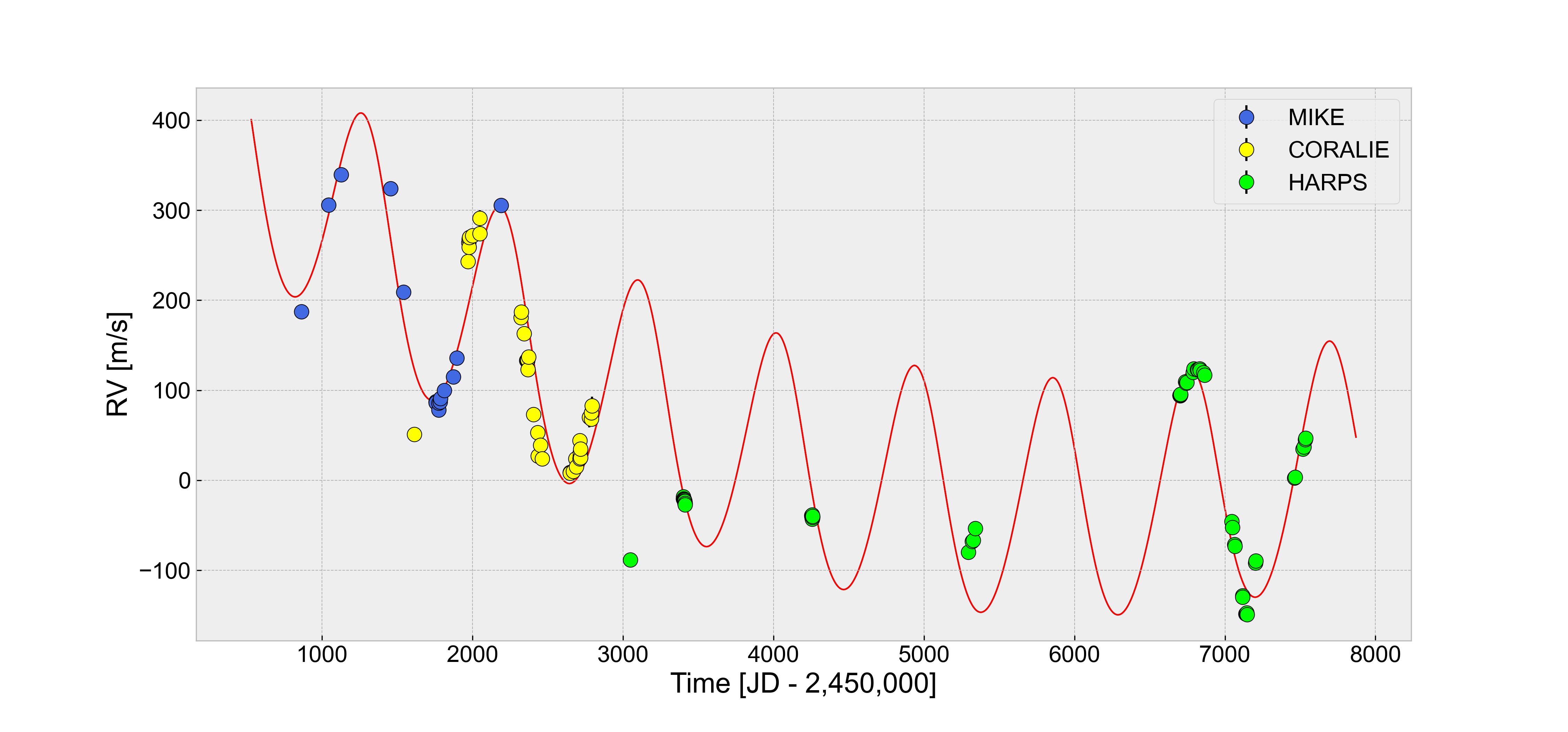
The star was also observed by Minniti et al. 2009 with the MIKE spectrograph as part of the Magellan Planet Search Program. Their independent dataset provided strong confirmatory evidence for the planet. However, they did not fit the CORALIE and MIKE data simultaneously. Had they done so, they would have found that the combined dataset is incompatible with a single-planet solution. Additional data from the HARPS public archive prepared by Trifonov et al. 2020 confirms this conclusion. Figure 7 shows all of the radial-velocity data.
The red curve is the best-fitting model involving a single planet and an ad hoc quadratic function of time. The model provides a decent qualitative description of most of the data, but the residuals show clear patterns and major outliers. In this model, days, which is closer to the Gaia-derived value of days than the originally reported periods of 1118 days (Minniti et al. 2009) and 1143 days (Mayor et al. 2004). The model’s eccentricity of is inconsistent with the Gaia-derived eccentricity of .
Clearly, there is more to this system than a star and a single giant planet. A joint fit was not performed because the results of such a fit would be incoherent. The star’s additional motion is obvious in the Doppler data and could also have affected the astrometric measurements over the 1000-day timespan of the Gaia observations.
IV.8 HD 114762
HD 114762 (BD18 2700, HIP 64426) is an early-G or late-F star at a distance of 39 parsecs, with . There are discrepant reports of its effective temperature: K (Kane et al. 2011), K (gspspec_teff), K (Ghezzi et al. 2010), K (Stassun et al. 2017), and K (gspphot_teff). Perhaps the differences are related to the star’s low metallicity [, per Kane et al. 2011, or , per Sousa et al. 2021]. The Gaia DR3 FLAME mass, , is adopted here.
HD 114762 played an important role in the history of exoplanetary science. Latham et al. 1989 found radial-velocity variations with a period of 84 days, an eccentricity of 0.3, and an implied of 11 Jupiter masses. The authors wrote that the companion was ‘a good candidate to be a brown dwarf or even a giant planet.’ Either discovery would have been the first of its kind.
The prolonged debate over whether the companion was likely to be an exoplanet took some interesting turns. Initially, it was unclear whether a giant planet could have such a high mass, high eccentricity, and short period. Of course, we now know of many giant planets with high eccentricities and short periods, and there are many objects with masses of 10–20 Jupiter masses that are classified as exoplanets in the NASA Exoplanet Archive.
By the early 2000s, the occurrence of short-period giant planets was known to be strongly associated with high metallicity (Santos et al. 2001; Fischer & Valenti 2005). This allowed another argument to be lodged against planethood for the companion of the metal-poor star HD 114762.
In addition, there was the generic problem common to all Doppler planets: the unknown inclination angle leaves open the possibility that the orbit is being viewed at low inclination, and is much larger than . In an attempt to constrain the inclination, Cochran et al. 1991 placed an upper bound of 1 km/s on the star’s projected rotation velocity, which is anomalously low for stars of the same spectral type. This suggested that the star’s rotation axis has a low inclination and — if the orbit is aligned with the star — the orbit is viewed nearly face-on. The premise of good alignment was reasonable at the time but was eventually undermined with the discovery of severe misalignments between stars and the orbits of short-period giant planets (see Albrecht et al. 2022, for a review).
Kiefer 2019 overcame the impasse using information from Gaia’s first data release. Although this data release did not include time-series astrometry, nor the results of two-body fits, it did report the ‘astrometric excess noise’, a measure of goodness-of-fit to a model in which the star has no companions. After performing simulations of possible orbits and the corresponding levels of astrometric excess noise that they would produce, Kiefer 2019 concluded that HD 114762’s orbital inclination is only 4–6∘ and the secondary mass is . Later, using DR3 data, Gaia Collaboration et al. 2022b and Holl et al. 2022 confirmed that HD 114762 is a face-on binary star.
Although the saga of HD 114762 b as a planet candidate has ended, a joint analysis of all the available data was performed for the sake of completeness. For this case, a minor change was made to the fitting procedure: the parameters and were used in the MCMC analysis rather than and . This is because for nearly face-on binaries, can be measured precisely even though and are degenerate.
Given the large quantity of Doppler data spanning more than 30 years, the parameters of the spectroscopic orbit are rigidly nailed down. The Doppler-only analysis gave days, m/s, and . These and the other Doppler parameters were found to be consistent with the Gaia DR3 two-body orbital solution. The joint fit does not exhibit any significant tension. The orbital inclination is degrees and the secondary mass is . One would expect a binary star to have a nonzero flux ratio, and indeed, the flux ratio was found to be .
Strong covariances exist between the uncertainties of the secondary mass, the orbital inclination, and the flux ratio, for the same reason that they were observed for HD 132406 (Section IV.3). To break this degeneracy, a simple mass-luminosity relationship was employed. The online version of Table 5 of Pecaut & Mamajek 2013 gives the absolute magnitude as a function of stellar mass. For masses between 0.15 and 1.1, the results are well described by a quadratic function,
| (18) |
where is the stellar mass (in solar masses) and the best-fit coefficients are = 14.14, , and .
The joint fit was repeated, this time with a Gaussian prior on the magnitude difference between the two stars with a mean determined by the application of Eqn. 18 to both stars, and a standard deviation of 0.25 (chosen somewhat arbitrarily). The prior constraint on the primary star’s mass was also loosened from to solar masses to allow for the possibility that light from the companion affected the classification of the primary star. The effect of these changes was to suppress the solutions with relatively high flux ratios. The inclination, secondary mass, and flux ratio found through this procedure were degrees, , and , respectively. The results are given in Table 3 and depicted in Figure 8, with the corner plot in the Appendix.

In this model, , remarkably close to unity. Only one out of 500 binaries in a randomly-oriented sample would be expected to have such a low inclination. Of course, HD 114762 was not drawn at random from such a sample. It drew attention because of the low amplitude of the Doppler signal, a selection criterion favoring face-on orbits.
| Parameter | Value | Value |
|---|---|---|
| # of | (no prior) | (with prior) |
| [] | ||
| [] | ||
| [days] | ||
| [days] | ||
| [rad] | ||
| [rad] | ||
| [mas] | ||
| [] |
Note. — The prior refers to a prior constraint on the relationship between the mass ratio and the flux ratio in the Gaia band. See Eqn. (18).
V Discussion
Exoplanetary systems that can be studied with more than one technique are especially valuable. The data from different techniques can validate and reinforce each other, while also providing more powerful constraints on the system’s parameters. At the moment, the most common combination is the pairing of the Doppler and transit techniques. The Doppler technique supplies , and the transit technique ensures while also giving access to the planet’s radius. According to the NASA Exoplanet Archive, there are 838 ‘confirmed’ planets that have been detected by both the Doppler and transit techniques. The next most common combination is that of the Doppler and astrometric techniques. Until very recently, almost all such systems were Doppler planets for which astrometric motion was detected with the Hubble Space Telescope Fine Guidance Sensors (Benedict et al. 2002; McArthur et al. 2010, see, e.g.,), or through the comparison of Hipparcos and Gaia positions and proper motions (Li et al. 2021). Prior to Gaia DR3, there were about 15 objects in this category, with the exact number depending on the upper mass limit chosen for planets. A few directly-imaged planets have also been detected with the Doppler method (Ruffio et al. 2021, see, e.g.,).
Now, astrometric information is available for 73 planets and candidate planets, of which 9 were already known to exist from Doppler surveys. Simulations of the Gaia survey suggest that 104 planets will eventually be detectable with Gaia data Perryman et al. 2014. Precise Doppler observations will play an important role in the validation and characterization of the planets with bright host stars, as emphasized by Gaia Collaboration et al. 2022b and Holl et al. 2022, and as demonstrated in this study.
For now, the publicly available Gaia information is limited to the results of fitting a two-body model to the data, rather than the time-series astrometry. When the Gaia orbital parameters have nearly Gaussian uncertainties and the star’s reflex motion is dominated by the effect of a single giant planet, there is no obstacle to combining the Doppler and Gaia information and obtaining good constraints on the three-dimensional orbit as well as the planet’s mass, as was the case for BD-17 0063, HD 81040, and HD 132406. In some cases, though, the interpretation of the data will be more difficult because of non-Gaussian uncertainties, as was the case for HD 175167 and HR 810, or the presence of multiple planetary signals, as is the case for HD 111232 and possibly for HIP 66074.
Progress is possible now, but much will have to wait until Gaia DR4 when the time-series astrometric data will become available. In the meantime, it would be useful to conduct long-term Doppler monitoring of stars known to have giant planets that are potentially detectable with Gaia. Too many giant planets have been discovered with the Doppler method and then ignored for a decade or more. Obtaining at least a little more Doppler data over timescales of a few years before DR4 would enhance our ability to interpret the Gaia data and make the most of the enormous exoplanet potential of the Gaia mission.
Appendix A Corner plots
Contained here are plots of the joint a posteriori probability distribution of the parameters for each system, based on the simultaneous fit to the Doppler data and Gaia orbital solution, and depicted as a ‘corner plot’ of 2-d distributions. The results for BD-17 0063, HD 81040, HD 132406, HIP 66074, HD 175167, HR 810, and HD 114762 are shown in Figures 9, 10, 11, 12, 13, 14, and 15, respectively.


References
- Albrecht et al. (2022) Albrecht, S. H., Dawson, R. I., & Winn, J. N. 2022, arXiv e-prints, arXiv:2203.05460. https://arxiv.org/abs/2203.05460
- Arriagada et al. (2010) Arriagada, P., Butler, R. P., Minniti, D., et al. 2010, ApJ, 711, 1229, doi: 10.1088/0004-637X/711/2/1229
- Babusiaux et al. (2022) Babusiaux, C., Fabricius, C., Khanna, S., et al. 2022, arXiv e-prints, arXiv:2206.05989. https://arxiv.org/abs/2206.05989
- Benedict et al. (2002) Benedict, G. F., McArthur, B. E., Forveille, T., et al. 2002, ApJ, 581, L115, doi: 10.1086/346073
- Butler et al. (2001) Butler, R. P., Tinney, C. G., Marcy, G. W., et al. 2001, ApJ, 555, 410, doi: 10.1086/321467
- Butler et al. (2017) Butler, R. P., Vogt, S. S., Laughlin, G., et al. 2017, AJ, 153, 208, doi: 10.3847/1538-3881/aa66ca
- Cochran et al. (1991) Cochran, W. D., Hatzes, A. P., & Hancock, T. J. 1991, ApJ, 380, L35, doi: 10.1086/186167
- Creevey et al. (2022) Creevey, O. L., Sordo, R., Pailler, F., et al. 2022, arXiv e-prints, arXiv:2206.05864. https://arxiv.org/abs/2206.05864
- da Silva et al. (2007) da Silva, R., Udry, S., Bouchy, F., et al. 2007, A&A, 473, 323, doi: 10.1051/0004-6361:20077314
- Fischer & Valenti (2005) Fischer, D. A., & Valenti, J. 2005, ApJ, 622, 1102, doi: 10.1086/428383
- Flores et al. (2017) Flores, M. G., Buccino, A. P., Saffe, C. E., & Mauas, P. J. D. 2017, MNRAS, 464, 4299, doi: 10.1093/mnras/stw2650
- Foreman-Mackey et al. (2013) Foreman-Mackey, D., Hogg, D. W., Lang, D., & Goodman, J. 2013, PASP, 125, 306, doi: 10.1086/670067
- Gaia Collaboration et al. (2022a) Gaia Collaboration, Vallenari, A., Brown, A. G. A., et al. 2022a, arXiv e-prints, arXiv:2208.00211. https://arxiv.org/abs/2208.00211
- Gaia Collaboration et al. (2022b) Gaia Collaboration, Arenou, F., Babusiaux, C., et al. 2022b, arXiv e-prints, arXiv:2206.05595. https://arxiv.org/abs/2206.05595
- Ghezzi et al. (2010) Ghezzi, L., Cunha, K., Smith, V. V., et al. 2010, ApJ, 720, 1290, doi: 10.1088/0004-637X/720/2/1290
- Goodman & Weare (2010) Goodman, J., & Weare, J. 2010, Communications in Applied Mathematics and Computational Science, 5, 65, doi: 10.2140/camcos.2010.5.65
- Halbwachs et al. (2022) Halbwachs, J.-L., Pourbaix, D., Arenou, F., et al. 2022, arXiv e-prints, arXiv:2206.05726. https://arxiv.org/abs/2206.05726
- Holl et al. (2022) Holl, B., Sozzetti, A., Sahlmann, J., et al. 2022, arXiv e-prints, arXiv:2206.05439. https://arxiv.org/abs/2206.05439
- Kane et al. (2011) Kane, S. R., Henry, G. W., Dragomir, D., et al. 2011, ApJ, 735, L41, doi: 10.1088/2041-8205/735/2/L41
- Kiefer (2019) Kiefer, F. 2019, A&A, 632, L9, doi: 10.1051/0004-6361/201936942
- Kürster et al. (2000) Kürster, M., Endl, M., Els, S., et al. 2000, A&A, 353, L33
- Latham et al. (1989) Latham, D. W., Mazeh, T., Stefanik, R. P., Mayor, M., & Burki, G. 1989, Nature, 339, 38, doi: 10.1038/339038a0
- Li et al. (2021) Li, Y., Brandt, T. D., Brandt, G. M., et al. 2021, AJ, 162, 266, doi: 10.3847/1538-3881/ac27ab
- Lindegren et al. (2021) Lindegren, L., Klioner, S. A., Hernández, J., et al. 2021, A&A, 649, A2, doi: 10.1051/0004-6361/202039709
- Marcy et al. (2001) Marcy, G. W., Butler, R. P., Fischer, D., et al. 2001, ApJ, 556, 296, doi: 10.1086/321552
- Mayor et al. (2004) Mayor, M., Udry, S., Naef, D., et al. 2004, A&A, 415, 391, doi: 10.1051/0004-6361:20034250
- McArthur et al. (2010) McArthur, B. E., Benedict, G. F., Barnes, R., et al. 2010, ApJ, 715, 1203, doi: 10.1088/0004-637X/715/2/1203
- Minniti et al. (2009) Minniti, D., Butler, R. P., López-Morales, M., et al. 2009, ApJ, 693, 1424, doi: 10.1088/0004-637X/693/2/1424
- Moutou et al. (2009) Moutou, C., Mayor, M., Lo Curto, G., et al. 2009, A&A, 496, 513, doi: 10.1051/0004-6361:200810941
- Naef et al. (2001) Naef, D., Mayor, M., Pepe, F., et al. 2001, A&A, 375, 205, doi: 10.1051/0004-6361:20010841
- NASA Exoplanet Archive (2019) NASA Exoplanet Archive. 2019, Confirmed Planets Table, IPAC, doi: 10.26133/NEA1
- Pecaut & Mamajek (2013) Pecaut, M. J., & Mamajek, E. E. 2013, ApJS, 208, 9, doi: 10.1088/0067-0049/208/1/9
- Perryman et al. (2014) Perryman, M., Hartman, J., Bakos, G. Á., & Lindegren, L. 2014, ApJ, 797, 14, doi: 10.1088/0004-637X/797/1/14
- Quirrenbach (2010) Quirrenbach, A. 2010, in Exoplanets, ed. S. Seager, 157–174
- Rosenthal et al. (2021) Rosenthal, L. J., Fulton, B. J., Hirsch, L. A., et al. 2021, ApJS, 255, 8, doi: 10.3847/1538-4365/abe23c
- Ruffio et al. (2021) Ruffio, J.-B., Konopacky, Q. M., Barman, T., et al. 2021, AJ, 162, 290, doi: 10.3847/1538-3881/ac273a
- Santos et al. (2001) Santos, N. C., Israelian, G., & Mayor, M. 2001, A&A, 373, 1019, doi: 10.1051/0004-6361:20010648
- Sanz-Forcada et al. (2019) Sanz-Forcada, J., Stelzer, B., Coffaro, M., Raetz, S., & Alvarado-Gómez, J. D. 2019, A&A, 631, A45, doi: 10.1051/0004-6361/201935703
- Sousa et al. (2021) Sousa, S. G., Adibekyan, V., Delgado-Mena, E., et al. 2021, A&A, 656, A53, doi: 10.1051/0004-6361/202141584
- Sozzetti et al. (2006) Sozzetti, A., Udry, S., Zucker, S., et al. 2006, A&A, 449, 417, doi: 10.1051/0004-6361:20054303
- Stassun et al. (2017) Stassun, K. G., Collins, K. A., & Gaudi, B. S. 2017, AJ, 153, 136, doi: 10.3847/1538-3881/aa5df3
- Strand (1943) Strand, K. A. 1943, PASP, 55, 29, doi: 10.1086/125484
- Trifonov et al. (2020) Trifonov, T., Tal-Or, L., Zechmeister, M., et al. 2020, A&A, 636, A74, doi: 10.1051/0004-6361/201936686
- Wittenmyer et al. (2012) Wittenmyer, R. A., Horner, J., Tuomi, M., et al. 2012, ApJ, 753, 169, doi: 10.1088/0004-637X/753/2/169