Ultra-Diffuse Galaxies as Extreme Star-forming Environments I: Mapping Star Formation in H I-Rich UDGsAstropy (Astropy Collaboration et al. 2013; Price-Whelan et al. 2018), matplotlib (Hunter 2007), SciPy (jon 2001), the IPython package (Pérez & Granger 2007), NumPy (Van Der Walt et al. 2011)
Abstract
Ultra-Diffuse Galaxies are both extreme products of galaxy evolution and extreme environments in which to test our understanding of star formation. In this work, we contrast the spatially resolved star formation activity of a sample of 22 H I-selected UDGs and 35 low-mass galaxies from the NASA Sloan Atlas (NSA) within 120 Mpc. We employ a new joint SED fitting method to compute star formation rate and stellar mass surface density maps that leverage the high spatial resolution optical imaging data of the Hyper Suprime-Cam Subaru Strategic Program (HSC-SSP) and the UV coverage of GALEX, along with H I radial profiles estimated from a subset of galaxies that have spatially resolved H I maps. We find that the UDGs have low star formation efficiencies as a function of their atomic gas down to scales of 500 pc. We additionally find that the stellar mass-weighted sizes of our UDG sample are unremarkable when considered as a function of their H I mass – their stellar sizes are comparable to the NSA dwarfs at fixed H I mass. This is a natural result in the picture where UDGs are forming stars normally, but at low efficiencies. We compare our results to predictions from contemporary models of galaxy formation, and find in particular that our observations are difficult to reproduce in models where UDGs undergo stellar expansion due to vigorous star formation feedback should bursty star formation be required down to .
I Introduction
Ultra-diffuse galaxies (UDGs) are dwarf galaxies that are characterized by large stellar sizes ( kpc) and low surface brightnesses ( mag arcsec-2, though exact definitions vary; see Van Nest et al. 2022 for an overview). These diffuse systems are extreme in two senses: they lie far above the mass-size relation, making them extreme products of galaxy evolution, but they are also extreme environments for star formation due to their low stellar surface densities.
UDGs as extreme products of galaxy evolution is a well-trodden topic both observationally (Sandage & Binggeli 1984; McGaugh et al. 1995; Dalcanton et al. 1997; van Dokkum et al. 2015; Beasley & Trujillo 2016a; Beasley & Trujillo 2016b; Peng & Lim 2016; Yagi et al. 2016; Leisman et al. 2017; van Dokkum et al. 2018; Danieli et al. 2019; Janowiecki et al. 2019; van Dokkum et al. 2019; Danieli et al. 2021; Gault et al. 2021, see, e.g.) and theoretically (Amorisco & Loeb 2016; Di Cintio et al. 2017; Chan et al. 2018; Greco et al. 2018b; Greco et al. 2018a; Jiang et al. 2019; Liao et al. 2019; Wright et al. 2021; Van Nest et al. 2022; Zaritsky et al. 2022, e.g.). However, the formation of the UDG population remains an open question. Several mechanisms have been proposed to form UDGs in the field, including stellar expansion from star formation feedback (El-Badry et al. 2016; Di Cintio et al. 2017; Chan et al. 2018), early mergers that trigger radial expansion of star formation (Wright et al. 2021), and preferential UDG formation in the high-spin tail of the halo distribution (Dalcanton et al. 1997; Liao et al. 2019).
It is observationally challenging to measure robust distances to UDGs due to their low surface brightnesses; as a result, the majority of UDGs with known distances are in clusters or groups. To understand the full breadth of the UDG population, of course, it is necessary to sample this population across a range of environments. Observational works continue to place new constraints on such mechanisms (Leisman et al. 2017; Greco et al. 2018b; Greco et al. 2018a; Janowiecki et al. 2019; Martín-Navarro et al. 2019; Gault et al. 2021; Kado-Fong et al. 2021; E Greene et al. 2022; Villaume et al. 2022, see, e.g.), but as of yet there has not been a clear convergence in the literature towards one path – of course, it is also not necessarily the case that all UDGs are formed via the same mechanism. Towards this end, there has been a push to use H I to detect and/or measure distances to UDGs (Leisman et al. 2017; Janowiecki et al. 2019; Karunakaran et al. 2020; Gault et al. 2021) – this allows for distance determinations in a sample of UDGs that tend towards low density environments.
It has been shown that although H I-selected UDGs lie on the star-forming main sequence and H I mass-size relation (Gault et al. 2021), they tend to have high H I masses (Leisman et al. 2017) – that is, the UDGs are, in an integrated sense, low in their star formation efficiency as a function of atomic gas, or SFE(H I). This in and of itself is not surprising – it has been demonstrated observationally that stellar mass surface density affects the position of dwarf galaxies with respect to the Kennicutt-Schmidt relation (Schmidt 1959; Kennicutt 1989) in that lower stellar mass surface density dwarfs lie below the main relation (de los Reyes & Kennicutt 2019). What has not yet been ascertained, however, is whether the apparently low SFE(H I) of the UDGs is a product of their selection, the distribution of their star formation, or a true physical suppression of SFE(H I).
In order to understand the origin of the low SFE(H I) of the UDGs, we introduce a joint SED fitting method that utilizes the spatial resolution of the optical Hyper Suprime-Cam Subaru Strategic Program (HSC-SSP) and the crucial UV coverage of GALEX. We use this method to derive stellar mass and SFR maps of a sample of H I-selected UDGs from Janowiecki et al. 2019 and a reference sample of H I-detected galaxies from the NASA Sloan Atlas (Bradford et al. 2015). We then use these maps, along with estimated H I radial profiles, to probe the star formation efficiency of these dwarfs down to 500 pc scales. In this work, our main focus will be on characterizing the properties of the H I-selected UDGs with respect to the “normal” NSA dwarf sample through a lens aimed largely at galaxy evolution. In Kado-Fong et al. 2022 (hereafter 44) we will shift our focus towards understanding star formation in H I-rich UDGs, with a particular focus on the role of UDG structure in the pressure-regulated, feedback-modulated model of star formation (Ostriker et al. 2010; Kim et al. 2011; Ostriker & Shetty 2011; Kim et al. 2013; Kim & Ostriker 2015; Kim et al. 2017).
II Datasets
Our dwarf sample consists of two main branches: a high surface brightness, “normal” dwarf sample drawn from the H I catalog of Bradford et al. 2015 – hereafter the NSA sample, and an ultra-diffuse galaxy sample with known distances from the H I catalog of Janowiecki et al. 2019. The UDG sample is selected to have a maximum distance of Mpc; we enforce the same limit on the NSA sample. We note that in this work we will refer to the “normal” galaxy sample as the NSA sample, as these galaxies were not specifically chosen to exclude low surface brightness galaxies. Rather, their relatively high surface brightnesses are a result of the observational selection which lead to their inclusion in the NSA.
II.1 Sample Overview
Here we detail the basic physical properties of the UDG and NSA samples. The sample consists of 58 galaxies at distances less than 120 Mpc; 22 are UDGs from Janowiecki et al. 2019 and 35 are NSA galaxies from Bradford et al. 2015. All sources are required to have clean 5-band HSC imaging, and all sources have measured H I masses and redshifts due to their selection method. The sample of Janowiecki et al. 2019 is not explicitly chosen to be in the field (in contrast to Leisman et al. 2017), but they find that the properties of their H I-selected UDGs are largely unchanged by environment. We find that one UDG in our sample, AGC227965, is quenched (SFR M⊙ yr-1) due to being a close satellite of MRK1324. We leave this galaxy in our analysis as it still yields a significant H I detection, but note that our discussion of the field UDG formation pathways does not apply to this system.
In Figure 1 we show our sample galaxies in stellar mass versus H I mass (left), SFR versus H I mass (center), and the star-forming main sequence (SFMS, right). These results are from a customized SED fitting method that we describe in detail in Section III, but can be thought of as standard SED fitting results for the purposes of the figures in this section. In this figure and all subsequent figures, we show the NSA sample in purple and the UDG sample in red. The NSA sample reaches higher stellar masses and lower H I masses than does the UDG sample; when noted, we compare only NSA galaxies with stellar masses within the observed range of the UDG sample. The results of the Leroy et al. 2008 sample of nearby galaxies and SDSS spectroscopic value-added catalog (Kauffmann et al. 2003; Brinchmann et al. 2004; Salim et al. 2007) are shown in beige and grey, respectively. We see that the UDGs have high H I masses for their stellar masses and that they have low SFRs for their H I masses – conversely, the UDGs lie directly on the SFMS.
A clear question arises from this initial analysis: are the H I-selected UDGs truly drawn from a more H I-rich population than the NSA dwarfs, or are the higher H I masses simply an effect of observational selection? To test this, we consider what our expected distribution of UDG H I fractions, , would be given the 21cm flux limit of the UDG sample if the distribution of the UDGs were the same as the NSA sample. To put it another way, we ask the following question: if the UDG population had the same distribution of H I fractions as the NSA dwarf sample, what is the distribution of that we would expect to see from an H I-selected sample?
We show the results of this test in Figure 2. The top panel shows the observed 21 cm line fluxes in solid points (as always, purple for the NSA sample and red for UDGs), while the unfilled red points show the expected 21 cm flux for each UDG in the sample if the H I fraction were drawn from the NSA dwarf distribution over . The errorbars in this panel are generated via bootstrap resampling from the NSA distribution. We estimate the detection limit of the UDG sample in two ways: first, from the stated completeness limit of the ALFALFA survey for sources with (Haynes et al. 2011, black dashed line), and second, from the lowest 21 cm flux of the UDG sample (red solid line). These limits are in good agreement with one another, and we adopt the minimum 21 cm line flux of the UDG sample as our detection limit for this exercise. The bottom panel of Figure 2 shows the distribution of observed H I fractions for the NSA (solid purple histogram) and UDG (unfilled red histogram) samples, as well as the UDG sample that we would expect to have detected if the UDG distribution over were the same as that of the NSA sample (hatched dashed red histogram). Indeed, we find that we would expect to detect a significant number of UDGs, should they exist. Rather, the marked H I richness of the UDG sample cannot simply be attributed to observational limits.
We extend this positioning of H I-rich UDGs as unusual star-forming environments by considering a globally averaged stellar mass, H I, and SFR surface density in Figure 3. In this figure, we compute using the total H I mass and the total area (as defined by the global elliptical HSC-g aperture, which we will describe Section III). One can immediately see that, as expected from their definition, the UDGs have significantly lower SFR and stellar mass surface densities than the NSA sample. Intriguingly, however, the UDGs do not also show signs of lower H I surface densities. Indeed, their H I surface densities span the same range as their spectroscopic counterparts.
The main thrust of this paper will be to root out the physical culprits of this apparently lowered SFE(H I). From globally averaged measurements alone, it is unclear whether the low average star formation rate surface density is a result of a truly lower SFE(H I), or whether the spatial distribution of star formation in UDGs differs from normal dwarfs (e.g. a low globally averaged could arise from an old stellar population that is significantly more extended than the star-forming regions). In order to distinguish between these two scenarios, we must build an SED fitting method to constrain local (500 pc scale) SFR and stellar mass surface densities (Section III) – we will return to this narrative of star formation efficiency in Section V.

II.2 UV-Optical Imaging
HSC-SSP. The HSC-SSP imaging boasts wide spatial coverage, high sensitivity (a point source depth of in its shallowest “Wide” layer), and high spatial resolution (the worst-seeing band, , has an average seeing of 0.77″).
For this work, we use the internal data release S21A, which covers 670 deg2 in 5 optical bands. The HSC-SSP data products include two options for the background subtraction – a local subtraction suited for small, high redshift sources, and a global subtraction suited for nearby galaxies. We use the coadd/bg versions of the co-added HSC images, which uses the “global” background subtraction of the S18A and PDR2 data releases (for an in-depth discussion of the HSC global background subtraction scheme, see Section 4.1 of Aihara et al. 2019 and Li et al. 2021). The data have been shown to reach surface brightness limits of mag arcsec-2 for radially averaged measurements around a known target (Huang et al. 2018; Kado-Fong et al. 2020).
GALEX. To complement the deep and high resolution optical imaging of the HSC imaging, we draw upon archival GALEX imaging to measure global UV photometry of our galaxies. We use the package astroquery to query the Barbara A. Mikulski Archive for Space Telescopes (MAST) for GALEX FUV and NUV observations that cover the position of each galaxy. We adopt the average GALEX PSFs in this work; the FUV and NUV PSFs have full widths at half maximum (FWHM) of 4.2’’ and 4.9’’, respectively11 1 http://www.galex.caltech.edu/researcher/techdoc-ch5.html. We measure our GALEX photometry on the background-subtracted intensity maps provided by the GALEX pipeline, and estimate uncertainties assuming Poisson noise for the counts.
For targets with more than one GALEX archival image, we prefer the data product with a longer total exposure time. Two NSA galaxies (NSA ID 5109 and 30738) do not have FUV imaging; all galaxies have NUV imaging. Of our sample with FUV imaging, 13 galaxies are drawn from the GALEX All-Sky Imaging Survey (AIS, ) and 35 from the Medium Imaging Survey (Martin et al. 2005, MIS, ,). 13 are drawn from guest investigator (GI) programs; we make an estimate the depth of the GI programs by measuring the standard deviation of random apertures of apertures the size of the average GALEX FWHM. The GI imaging is somewhat deeper than the MIS imaging, with a mean depth of . Similarly, 6 galaxies in our sample have NUV AIS imaging, 40 have MIS imaging, and 9 have GI imaging. We repeat the same procedure to estimate the depth of the GI imaging and find a mean depth of . We note that the depths estimated here are not used in the analysis, and are simply meant to contextualize the GALEX imaging sources for the reader.
II.3 H I Measurements
All of the galaxies in the present work have integrated H I measurements from Janowiecki et al. 2019 or Bradford et al. 2015. However, resolved H I measurements exist only for a small subset of the UDGs identified by Janowiecki et al. 2019 – 12 from Gault et al. 2021, 3 from Leisman et al. 2017.
To estimate the radial profiles of the H I in our UDG and NSA dwarf samples, we leverage the empirical result that UDGs and “normal” dwarfs are similar in their H I structure – that is, UDGs lie on the H I mass-size relation and have typical average H I surface densities (Gault et al. 2021). We use this result to estimate Sérsic profile parameters for our sample via a parameter estimation from the spatially resolved measurements of Hunter et al. 2021 (who report Sérsic parameter fits for their sample), as well as the spatially resolved measurements of the UDGs in Gault et al. 202122 2 here we solve for the Sérsic parameters of their galaxies using the given measures of H I structure. We perform a least squares fit to the Sérsic index, , central surface density, and effective radius, , of the literature samples as a function of H I mass; only shows a significant correlation with H I mass (i.e. the H I mass-size relation). This allows us to estimate Sérsic parameters for our galaxies as a function of their H I mass. As these structural measures are not well-constrained, we will account for the uncertainties induced by our estimated H I profiles to demonstrate to the reader that these estimates are indeed reasonable.
First, although the Sérsic profile has three free parameters, our knowledge of the total H I mass allows us to determine the value of one of these parameters given estimates for the other two. We therefore choose to fix the H I central surface density via the analytic solution for the total H I mass of a 1D Sérsic profile, i.e.:
| (1) |
We find that the values derived from a fit to the literature data and the values derived using the total H I mass are in good agreement, with the latter method resulting in values that are on average higher than the former.
Second, to account for the substantial uncertainty induced by our lack of spatially resolved H I, we include an uncertainty in the parameter estimation of the Sérsic profiles equivalent to the standard deviation of the literature parameter values for reference (literature) galaxies within 0.5 dex of that of the target (NSA/UDG) galaxy in total H I mass. If no galaxies are sufficiently close in H I mass, we increase the tolerance from 0.5 dex to up to 0.9 dex, but note that because the reference sample of Hunter et al. 2021 is systematically lower mass than our sample, this only affects the most massive () galaxies in our sample. We then estimate the uncertainty on the radial H I surface density profile via Monte Carlo resampling assuming that the uncertainties are well-describe by normal distributions.
The resulting H I surface density profiles are shown in Figure 4; as above, red curves indicate UDGs and purple curves indicate NSA galaxies. The shaded regions span the 16th to 84th percentiles of the Monte Carlo simulation result for each galaxy. The directly measured H I profiles of Leroy et al. 2008 are shown in green, while the Sérsic profiles inferred from the structural measurements of Gault et al. 2021 are shown in orange. We find that our inferred profiles are in good agreement with the shape, normalization, and scatter of the directly measured profiles, with the exception of one UDG (AGC238764, which is not a part of our sample) that has an anomalously high Sérsic index (; almost all dwarfs in this mass range are characterized with sub-exponential Sérsic indices, see Hunter et al. 2021). There is, to our knowledge, only one H I-rich UDG that has spatially resolved H I data at a high enough resolution to probe the clumpiness and substructure of the H I (Mancera Piña et al. 2022). These data, which have a physical beam size of kpc, show significant H I substructure that is not captured in our simple radial profile estimation approach. However, the deviations from the radial profile that these azimuthal variations cause are comparable to the uncertainty we have already attributed to our radial profiles (see right panel of Figure 1 of Mancera Piña et al. 2022). We thus find it unlikely that we are overestimating the precision of the H I profiles, though we of course note that obtaining high resolution H I maps would dramatically improve the precision and accuracy of our estimates.


III SED Fitting
The key technical challenge of this work is inferring the star formation and stellar mass properties of the dwarf sample at sub-galactic scales. We accomplish this by modeling the high spatial resolution HSC optical data in conjunction with the UV GALEX measurements to constrain star formation activity in a consistent way with the UV data.
The novelty of our approach is to leverage both the high spatial resolution of HSC and the expanded wavelength coverage of GALEX to infer local star formation surface density properties of our dwarfs via a joint fit to localized optical photometry and global UV photometry. Here, we detail the fitting process employed in this work.
III.1 Stellar Population Models
We use the Flexible Stellar Population Synthesis (FSPS) models (Conroy et al. 2009; Conroy & Gunn 2010) with a fixed stellar and gas-phase metallicity of along with a Kroupa 2001 initial mass function to generate our synthetic spectra. We choose a single value for the model metallicity as the mass-metallicity relation is not well-understood for these dwarf samples. Direct () measurements of nearby dwarfs (Lee et al. 2006; Berg et al. 2012; Jimmy et al. 2015) can show significant offsets relative to each other and to metallicity estimates from SED fitting to more distant dwarf samples (Bellstedt et al. 2021). We thus choose to adopt a typical value following the literature compilation of (Bellstedt et al. 2021) for a galaxy of . We also check the impact of adopting solar metallicity models in Appendix B, and find that our SED fitting results are shifted by less than dex on average. The library includes nebular emission, which may contribute significantly to the broadband flux of the dwarf galaxies in our sample. We adopt an exponentially declining star formation history
| (2) |
We choose this relatively rigid star formation history (two free parameters, the onset of star formation and the timescale of decay ) in order to achieve reasonable computation times when the number of regions to be fit is high. Such a rigid choice of the SFH functional form has the potential to bias SFH recovery, and so we note that the main goal of our analysis is to diagnose the relative change in star formation surface density and star formation efficiency between normal, high surface brightness dwarfs and ultra diffuse galaxies, not to provide comprehensive stellar population synthesis properties for the UDGs. We will return to this point more comprehensively in Section IV when we consider validation tests for this method.
The composite stellar population (CSP) model library spans ages between 2 Myr and 12 Gyr and timescales () between 0.3 Gyr and 10 Gyr. Each axis consists of 50 logarithmically spaced values. We pre-compute both the UV-optical spectra and the fluxes through the GALEX and HSC bands for each model in the library. During fitting, we linearly interpolate between pre-computed library fluxes to obtain the predicted GALEX and HSC fluxes for arbitrary choices of and . Because we use pre-computed library fluxes at a fixed distance of 10 Mpc, this induces a small k-correction error in the galaxy sample. However, the most distant galaxies in our sample are at 120 Mpc, and so the k-correction error induced is negligible.
III.2 Defining Global, Regional, and Cluster SEDs
The first step to executing a joint fit between the optical and UV photometry is to establish the apertures in which we measure the optical and UV photometry. To obtain consistent optical photometry, we PSF match the HSC imaging with the worst seeing. To do so, we use the Fourier transform-based implementation of photutils with a cosine bell window function () to compute matching kernels between the other optical bands and the band to which we will match the PSF. We model the PSFs measured by the HSC pipeline (which produces PSF postage stamps with spatial extents of about 7″) as two-dimensional Moffat functions. We choose to simplify the PSF model to Moffat functions in order to prevent the emergence of imaging artifacts during the matching process caused by high frequency features in the original pipeline-produced PSFs. We additionally correct for galactic extinction in all UV and optical photometry presented in this work using the measurements of Schlafly & Finkbeiner 2011 via the associated online service (IRSA 2022).33 3 Galactic extinction measurements were accessed via https://irsa.ipac.caltech.edu/applications/DUST/
We then define the global aperture of the galaxy using sep, a python implementation of the segmentation algorithm used in SExtractor (Bertin & Arnouts 1996). In all cases, we use the HSC-g band as the detection band, with a detection threshold of 5 over the variance image supplied by the HSC pipeline. We define the elliptical global aperture as
| (3) |
where and are the light-weighted central coordinates of the galaxy and , , and are the standard SExtractor ellipse parameters
| (4) |
where and are the semi-major and semi-minor axes, respectively, and is the position angle of the galaxy measured counterclockwise from the horizontal (in image coordinates). This global aperture step is shown visually in step b of Figure 5 – the global aperture defined in step b using the optical data is then applied to the UV imaging to derive the global UV SED (step d). We choose not to PSF match the optical data to the UV data to maintain the spatial resolution of the optical data in order to hold the input images consistent between the global and spatially resolved SED fitting. If we did perform PSF matching to the GALEX imaging to compute the global optical photometry, we have verified that the changes would be negligible, with a mean fractional deviation in flux of 0.03 and a standard deviation of -0.02.
Next, to define the regional boundaries for the optical photometry, we lay a grid of fixed size over the cutout image, as shown in step e of Figure 5. The box length of this grid is set to be no less than twice the FWHM of the PSF-matched images, and is increased iteratively until the median SNR of the SEDs measured in the regions is at least 3. To remove regions where a reliable SED cannot be measured at the required spatial scales, we remove the bottom 5% faintest regions. We also mask regions with and generate additional masks for the UDGs, whose diffuse structure and large on-sky sizes make standard deblending routines unreliable. We verify that this pruning does not affect the total inferred mass and star formation rate in Section IV.
Because the size of the regions is small compared to the size of the galaxy, it is unsurprising to note that many of the regional SEDs are identical to each other to within their photometric errors. To decrease the number of parameters to fit, and to increase the SNR of the SEDs that we fit, we group the regions (step e) into clusters of similar SEDs (step f). We group the regions into clusters using K-means clustering, initially with 3 clusters. If any cluster has a SNR, we combine the low-SNR cluster with the closest high-SNR cluster (here defining closeness by the norm44 4 Where the -norm is the difference between the SED flux and reference flux over the optical bands over the optical SEDs). Next, we must verify that the cluster SEDs adequately represent their input regional SEDs. We use the metric , where is the flux in band measured in region , while is the flux in band measured in cluster . and refer to the uncertainty on the respective flux measurement. We impose the condition for all bands and all regions assigned to cluster for each cluster in the galaxy. If the clustering result fails this verification, we rerun the clustering process with an additional cluster at the K-means step. We allow up to five clusters, at which point the clustering assignment is accepted regardless of verification status. In practice, only one galaxy (the UDG AGC223246) is fit with the maximum five clusters.
III.3 SED Fitting
With our PSF-matched photometry and apertures in hand, we are now ready to begin the SED fitting. For all of our fitting, we use the Markov Chain Monte Carlo implementation of emcee (Foreman-Mackey et al. 2013). We adopt a flat prior over positive values for the amplitude of each cluster SED, a flat prior between 0 and 13.6 Gyr for (see Equation 2), and a log-normal prior over distributed as . In our joint fitting step, where multiple amplitudes and values are being inferred, the prior is the same for each individual parameter.
We first perform a global SED fit using both the optical and UV photometry to constrain the reddening, , and to provide an estimate of the total stellar mass and star formation rate. We adopt a Gaussian likelihood, defined as:
| (5) |
where refers to the flux of the band out of bands ( for our fiducial case), is the predicted model flux, and is the uncertainty in the band. We measure directly from the variance images of HSC-SSP added in quadrature to an extra uncertainty of . In this step we run emcee for 1500 iterations with 32 walkers, discarding the first 400 steps. The only parameter from this fit that survives as a final result is the reddening, which is used to the joint fit as a fixed parameter. We find no difference in the estimated for the UDGs and the NSA galaxies at : the 50th (16th and 84th) percentile of the distribution is (0.04, 0.37) for the UDGs and (0.05, 0.38) for the NSA dwarfs at . Unsurprisingly, the NSA galaxies at higher stellar mass have systematically higher estimated reddening – (0.55, 0.99).
Next, we compute the flux in the SED clusters defined as above. At this stage, the model consists of a set of models across bands. The likelihood is computed as follows:
| (6) |
where refers to the bandpass index and refers to the cluster index. In other words, we retain a Gaussian likelihood wherein the UV bands (FUV and NUV) are compared against the sum of the regional models, whereas the optical bands ( in Equation 6; g,r,i,z, and y) are compared against the appropriate regional models. In this step, the walkers are initialized with the positions drawn from the posterior of the global SED fit; the amplitude of each cluster SED is additionally multiplied by the mean ratio between the flux in the cluster SED and the global SED over the optical bands. In this step, we run emcee for 20000 iterations with at least 32 or walkers, discarding the first 5000 steps.
From this process we estimate the total stellar mass and star formation rate for each cluster SED. We then convert these to stellar mass and star formation rate surface densities assigned to each regional SED by multiplying by the ratio of the flux in the regional SED and the flux in its corresponding cluster SED, and dividing by the physical area subtended by the region.
We show an example of the fitting procedure for the galaxy NSA 5449 in Figure 6. We also show an abbreviated gallery of fitting results in Appendix A for a set of galaxies that span the morphologies seen in the NSA and UDG samples.
IV Method Validation
In order to apply the framework constructed in the previous section to our galaxy samples, we must first take the necessary step of validating that our method is able to accurately deliver the quantities of interest to this study – namely, maps of the star formation and stellar mass surface densities down to the spatial resolution of HSC.
An equally important step is to lay out the quantities that we are not attempting to constrain with this modeling. The age, stellar metallicity, and detailed (flexible) star formation history of the galaxies are all parameters that may be estimated from SED fitting. However, it has been shown that the exponentially declining tau model is an imperfect model of star formation histories at large, both due to its overall rigidity and that it, by definition, ties early and late star formation (Simha et al. 2014; Carnall et al. 2019). Thus, we stress that our main goals, and the subjects of our verification tests, will be the estimation of the star formation rate and stellar mass surface densities, and not a detailed interrogation of the star formation history and enrichment of the galaxies in our sample.
IV.1 Intra-sample Comparisons
We first consider an internal comparison between the star formation rate and stellar masses measured from the global UV+optical SED fitting (step b and step d of Figure 5) and the integrated star formation rate and stellar masses obtained by summing the properties inferred from the cluster SED fitting (step f). In Figure 7, we show the integrated estimates of stellar mass (top) and star formation rate (bottom) for the UDGs (red) and NSA galaxies (purple). In all cases, we find good internal consistency between the initial SED fit on the global photometry and the final model SED of the spatially resolved method.
We additionally compare the stellar mass and SFR estimates obtained from our spatially resolved SED fitting method to the catalog NSA stellar masses and FUV-only SFRs in Figure 8. The FUV-only SFRs are computed from the catalog GALEX measurements using the prescription of Kennicutt 1998, i.e.
| (7) |
Both the catalog stellar mass estimates and the FUV-only SFRs are also in good agreement with the results of our spatially resolved fit.
Although we lack truly spatially-resolved spectroscopic measurements for the galaxies in our sample, we do have access to one quasi-resolved measurement for the NSA sample – the SDSS 3” fiber spectra. Because our galaxies exceed the SDSS fiber size, the SDSS spectroscopic measurements do contain information about the spatial distribution of star formation within the galaxy, albeit in a very limited capacity. In the right panel of Figure 8 we show a comparison between SFRs derived from the SDSS fiber spectroscopy of the NSA galaxies and SFRs we compute by integrating our SFR maps over SDSS-like apertures. The SDSS spectroscopy we reference are 3” diameter fiber spectra; we use the NSA catalog line fluxes in this comparison. In particular, we use the catalog H flux to compute H-derived star formation rates within the SDSS aperture following Calzetti 2013 with a Kroupa 2001 IMF:
| (8) |
Although the 100 Myr averaged SFRs we produce via our SED fitting are not completely analogous to the H SFRs derived from the SDSS spectra (which probe timescales closer to Myr), we expect that the two should be well-correlated. Indeed, we find that the star formation rates we compute from the central three arcseconds of our star formation rate maps are in good agreement with the SDSS spectroscopic measurements, with a scatter on the same order as the physical variation between UV and H SFRs measured from Local Volume dwarfs (Karachentsev et al. 2021, red line in right panel).
IV.2 Inter-sample Comparisons to the Literature
We also find good agreement between our results and literature measures of the integrated stellar mass, SFR, and for the two low surface brightness galaxies presented in Greco et al. 2018a, though we do not include these galaxies in this work because they lack H I measurements.
Finally, we compare to spatially resolved measurements of stellar mass, SFR, and H I in nearby samples of dwarfs from the literature. In Figure 9, we show a comparison between radial profiles of stellar mass surface density (left) and SFR surface density (right) as derived from our SED fitting method as compared to the directly measured results of Leroy et al. 2008. Our results are shown as solid curves, the Leroy et al. 2008 profiles are shown as dashed curves; all curves are colored by total stellar mass. Encouragingly, we find good agreement in both the shape and normalization between our inferred radial profiles and the directly measured results of Leroy et al. 2008, indicating that our method is able to recover not just the total amount of stellar mass and SFR, but the distribution of these quantities.

| ID | RA | Dec | Dist | SFR | |||||
|---|---|---|---|---|---|---|---|---|---|
| [deg] | [deg] | [Mpc] | [] | [] | [] | [mag] | [kpc] | [kpc] | |
| NSA16938 | 140.433 | 4.374 | 85.81 | ||||||
| NSA11919 | 132.078 | 1.263 | 27.67 | ||||||
| NSA16993 | 143.969 | 4.017 | 81.05 | ||||||
| NSA13797 | 174.755 | 1.336 | 24.92 | ||||||
| AGC334353 | 345.863 | 1.704 | 71.40 | ||||||
| AGC334349 | 345.277 | 1.998 | 51.10 | ||||||
| AGC103435 | 3.838 | 1.075 | 28.50 | ||||||
| AGC198540 | 141.308 | 3.313 | 63.30 |
Note. — Table 1 is published alongside this article in its entirety in the machine-readable format. A portion is shown here for guidance regarding its form and content.
V Results
With our methodology in hand, we may now return our focus to the physical question at hand. In Section II.1, we demonstrated that although the UDGs have low globally averaged stellar mass and SFR surface densities, their H I surface densities are comparable to those of the NSA galaxies. Now, we can consider the cause of the low SFE(H I) of the UDGs – and in particular whether this inefficiency persists to sub-kpc scales – as well as the relationship between UDG structure and H I content. For the interested reader, we include a table of selected SED fitting results for the sample in Table 1.
V.1 The Efficiency and Distribution of Star Formation in UDGs
In the top row f Figure 10, we show the relation between the estimated and at 500 pc, 1 kpc, and global scales from left to right (we note that, for reasons of visual continuity, the bottom right panel of Figure 10 is identical in content to the bottom panel of Figure 3). We compute 1 kpc and 500 pc average stellar mass surface density and SFR surface density maps by placing a grid of length 1 kpc or 500 pc (at the distance of the galaxy) over the stellar mass and SFR maps produced via SED fitting. We do not compute average quantities over length scales less than the regional SED box size for each galaxy. For the 1 kpc and 500 pc regions, the H I surface density is estimated using the central position of the region and the Sérsic profile estimated for the galaxy as described in Section II.3. From this figure, the reader may immediately notice that the shift in persists down to 500 pc; there are no regions in the area-weighted census of the UDG distribution of SFR surface density that match the vigorously star-forming SFR surface densities observed in the NSA dwarfs.
The persistence of the discrepancy of star formation activity outcomes as a function of H I surface density indicates that it is not simply a matter of the distribution of star formation that drives the apparently low star formation efficiency (as a function of atomic gas) in the UDG sample. Rather, it appears to be a generic property of star formation in our sample of UDGs. The question, then, of whether a more comprehensive understanding of star formation can explain this low star formation efficiency will naturally arise to the reader. This question is the central topic of 44, in which we will examine the impact of the UDGs’ peculiar stellar structure on their star formation activity within the framework of pressure-regulated, feedback-modulated star formation (Ostriker et al. 2010; Kim et al. 2011; Ostriker & Shetty 2011; Kim et al. 2013; Kim & Ostriker 2015; Kim et al. 2017).
We note that the minimum region size over which we can measure and is set by the distance of the galaxy and the angular scale over which we measure our regional SEDs (panel e, Figure 5). In particular, the galaxies for which we are able to measure 500 pc averages tend to be the closest galaxies in our samples, and are thus skewed towards lower stellar masses. However, we find that this effect does not impact the results presented here, as the majority of galaxies affected are more massive than the UDGs in this sample. In particular, there are five galaxies within the stellar mass range of the UDGs that are affected. Four are themselves UDGs (AGC 227965, AGC 322019, AGC 198543, and AGC 238961), and one is a NSA dwarf (NSA ID 17750).
V.2 The H I Properties of the UDG Sample
In addition to their star formation efficiency, it is of interest to understand the relationship between the stellar structure of these H I-rich UDGs and their integrated gas properites. In Figure 11, we show the mass-size relation of the UDG and NSA samples for two definitions of “mass” and “size” (i.e. four total combinations). The left column shows sizes measured as g-band half-light radii, while the right column shows sizes measured as half-mass radii, where we refer to the radius that contains half the stellar mass of the galaxy as the half-mass radius. The half-light, half-mass, and half-SFR radii reported in this work are measured over the same area of the galaxy as our derived stellar mass and SFR maps (i.e. only in pixels where the stellar mass surface density is nonzero). We use the PSF-matched HSC images with the same machinery as the half-mass and half-SFR radius measurement. The half-light radii reported in this work are thus not completely analogous to effective radii measured using other methods (e.g. Sersic fitting). In particular, though there is no systematic offset between the two methods ( for the full sample, and -0.06 (-0.04) for the NSA (UDG) subset), there is significant scatter ( for the full sample, and 0.13 (0.19) for the NSA (UDG) subset). We estimate the uncertainty in our half-mass and half-light radius measurements by adding in quadrature the physical size of the PSF FWHM and the standard deviation of the radii due to the uncertainty in the stellar mass fits/photometry, respectively. The top row shows H I mass, while the bottom shows stellar mass. In essence, one can think of the bottom left panel as the “canonical” mass-size relation (stellar mass versus light-weighted size).
When one considers the size of the UDGs as a function of their integrated stellar mass, it is immediately apparent that they are systematically larger than the NSA sample in both their light-weighted and mass-weighted sizes. This is unsurprising, of course, given that UDGs are selected for their low surface brightnesses and large physical sizes. When one considers the UDGs as a function of their integrated H I mass, however, the picture changes. In particular, we see no significant difference in the relation between the H I masses and half-mass (stellar) radii of the UDG and NSA samples. There is, however, some evidence that the half-light radii of the UDGs remain elevated with respect to the NSA sample at fixed H I mass.
V.3 The Color-Mass Relation of UDGs
Though not the main focus of this work, we are able to directly compare the color-mass relation of gas-rich UDGs and “normal” dwarfs as a byproduct of the SPS fitting presented above. Standard color-mass relations (Bell et al. 2003; Into & Portinari 2013, e.g.) have been assumed in the literature for color-based estimates of UDG stellar mass (Mancera Piña et al. 2019a; Karunakaran et al. 2020; Marleau et al. 2021, cf), but it has not been directly shown that these optical color relations are applicable to the UDG population. In particular, the canonical color-mass relations are typically calibrated for and tested on largely massive galaxies; it is thus of practical importance for both the UDG community and general dwarf galaxy community to test the applicability of these relations on the extreme pockets of the dwarf population (e.g. UDGs, Blue Compact Dwarfs, etc.).
In Figure 12 we show the global (i.e. light-weighted) g-band mass-to-light relations of the dwarfs in this work (as usual, red points indicate the UDG sample while purple points indicate the spectroscopic dwarf sample). We calculate stellar mass-to-light ratios by computing the luminosity and stellar mass from the global optical SED of each galaxy (panel b in Figure 5). The colors are measured using the same SED used to derive the stellar mass-to-light ratio.
We find that there is no offset between the H I-selected UDG sample and the NSA dwarf sample, and that the samples are well-described by a relation that lies between the Into & Portinari 2013 and Bell et al. 2003 color-mass relations. For completeness, we list our ordinary least squares parameters and standard errors here, where we define . We avoid the standard choice of as it is reserved for a parameter linking star formation and midplane pressure in 44.
| (9) |
the exact calibration of this relation is, of course, dependent on both the photometric bands used and IMF assumptions. We in particular note that Into & Portinari 2013 and Bell et al. 2003 are calibrated for SDSS g and r bands, which are similar but not identical to HSC g and r bands). Regardless, we have demonstrated that the UDGs do not lie systematically off of the color-mass relation of the NSA dwarfs, and that both samples are in relatively good agreement with previous relations from the literature.
VI Discussion
Taken altogether, we find that our sample of H I-rich UDGs are characterized by low star formation efficiencies (where SFE(H I) ) down to sub-kpc scales, and that the UDGs are generally incapable of supporting the vigorous star formation seen in the “normal” NSA dwarfs. Intriguingly, although the UDGs are large in light-weighted size for their total stellar mass, their stellar mass-weighted sizes are typical for their H I masses. Finally, the stellar mass-to-light ratios of the UDGs appear consistent with those of the NSA dwarf sample.
VI.1 Implications for UDG Formation
The results presented in this work suggest that the H I-rich Ultra-Diffuse Galaxies are unable to efficiently convert gas to stars or host vigorous star formation. Such low star formation rate surface densities indicate that UDGs will continue to trail behind the stellar mass build-up of the general dwarf population. This finding, however, does not alone answer the question of why certain galaxies fail to trigger vigorous star formation. Several mechanisms have been put forth in the literature to explain the population of field UDGs. For each formation model, we will first discuss the points in which our observations agree with the model predictions before turning towards points of potential conflict.
Feedback-driven expansion. We first consider the picture in which field UDGs are formed via starburst-driven outflows which cause potential fluctuations that in turn lead to net expansion of the stellar population (El-Badry et al. 2016; Di Cintio et al. 2017; Chan et al. 2018). We note to the reader that in this section we deal with results from both the Feedback In Realistic Environments (FIRE, Hopkins et al. 2014, and FIRE-2, Hopkins et al. 2018) and Numerical Investigation of a Hundred Astrophysical Objects (NIHAO, Wang et al. 2015) simulations; though both simulations point to feedback-driven expansion as the culprit of UDG formation, the feedback implementation between the two simulations is not identical.
In the NIHAO simulation, such UDGs are expected to retain systematically higher H I fractions with respect to “normal” dwarfs, in good agreement with our results (Di Cintio et al. 2017). However, two points of potential conflict emerge. First, the radial expansion of the UDG stellar population should enforce a radial age gradient; that is, the older stars should experience more expansion due to having gone through a larger number of inflow/outflow cycles. This picture suggest a relatively centrally concentrated distribution of star formation in UDGs, where the stars experience net expansion while the gas goes through cyclical phases of inflow and outflow. Such behavior is in qualitative conflict with the observation that UDG star formation is both consistently lower than and more radially extended than star formation in the NSA dwarfs (see lower panels of Figure 9). However, to our knowledge a detailed study of the star formation extendedness and efficiency has not been done for UDGs created by feedback-driven expansion. Further analysis is necessary to confirm that feedback-driven expansion cannot reproduce this effect (via, e.g. the substantial expansion of stars within 100 Myr of formation).
However, another point of conflict exists between our observations and the feedback-driven expansion picture. Namely, in both FIRE and NIHAO the marked expansion of the UDGs is driven by particularly prolonged and bursty star formation histories (Di Cintio et al. 2017; Chan et al. 2018). In this work, we have shown that the lack of vigorous star formation in UDGs is linked to their low stellar mass surface densities; that is, their low SFR surface densities are explainable by their stellar and gaseous structure. Conversely, then, the structure of the UDGs makes it difficult to envision a scenario in which they are able to power frequent and vigorous bursts of star formation at late times. This does not, of course, rule out UDG formation via star formation feedback if the star formation behavior of UDGs was markedly different at high redshift than it is in nearby UDGs. Indeed, such a transition has been predicted in models such as Trujillo-Gomez et al. 2022. However, these new observations provide new constraints on models which predict star formation feedback to remain vigorous down to .
Early mergers. Another proposed mechanism for field UDG formation is the result of an early merger (more than 8 Gyr ago) that caused an increase in total spin as well as a decrease in central SFR and a redistribution of star formation to large radii (Wright et al. 2021). Like our observed galaxies, the galaxies in the ROMULUS25 simulation are H I-rich for their stellar mass and lie on the integrated star-forming main sequence. However, we do not find the lower central specific star formation that Wright et al. 2021 cite as a significant observable manifestation of this formation channel; indeed, the distribution of sSFR of the UDGs in our sample is not statistically different than that of the NSA sample at any radius.
High-spin halos. Finally, we consider the proposal that UDGs are formed out of the high spin tail of the halo distribution (Dalcanton et al. 1997; Amorisco & Loeb 2016; Rong et al. 2017; Di Cintio et al. 2019; Liao et al. 2019, see, e.g.). This formation scenario predicts that UDGs will host ordered H I disks, in line with resolved measurements from the literature (Mancera Piña et al. 2019b; Mancera Piña et al. 2020; Gault et al. 2021). There is some suggestion that in this formation scenario, UDGs at should have generally lower central volumetric gas densities and more radially extended profiles than high surface brightness galaxies at fixed stellar mass (Liao et al. 2019). This may be at odds with observational findings, given that the UDGs in our sample have similar H I surface densities to the NSA dwarfs (see, e.g. Figure 10, which excludes NSA dwarfs with stellar masses larger than the range probed by the UDG sample) and have been previously suggested to lie on the H I mass-size relation (Gault et al. 2021). Together, these findings imply similar volumetric gas densities between the UDGs and NSA dwarfs if there is no systematic difference in disk thickness between the UDGs and NSA dwarfs. However, the relationship between UDG and normal dwarf H I disk thickness remains observationally uncertain. We thus underscore that we are not seeking to make a comprehensive comparison between the H I structural properties of observed UDGs and their simulated high-spin analogs.
The upshot of the discussion at hand, rather, is that neither the early merger scenario nor the high-spin halo scenario are in conflict with the most salient point of our analysis – that once set on a path towards low-efficiency star formation, galaxies like our present-day UDGs are likely to continue to fall behind the stellar mass build-up of the general dwarf population.
VI.2 The Stellar Structure of Dwarfs at fixed
In addition to a comparison with established theoretical models, it is informative to consider what fully empirical statement we may make about the relationship between the H I-rich UDGs and “normal” NSA dwarfs. In the preceding sections, we have demonstrated that the stellar half-mass radii of the UDGs are typical for their H I masses (see Figure 11) – that is, the UDGs are not offset from the mass-size plane for a particular casting of mass (H I mass) and size (stellar half-mass radius). This is contrasted, naturally, to the offset in the normal mass-size plane (stellar mass and half light radii) by which UDGs are definitionally characterized.
A concordance in the H I-mass-stellar-size relation would naturally arise if the UDGs were forming stars normally with respect to the spatial distribution of gas, but at decreased star forming efficiency. To illustrate this idea, let us presume that the spatial distribution of H I in UDGs is normal with respect to high surface brightness galaxies, as has been shown for a number of the UDGs in our sample by Gault et al. 2021. As hinted to in the introduction, the driving mechanism behind the low star formation efficiency of the UDGs will be further explored in 44.
In this picture, a galaxy that will become a UDG will form stars over the same spatial distribution as a galaxy that will become a high surface brightness galaxy, but at lower – thus becoming a galaxy with a lower total stellar mass. The concordance of the UDG and NSA samples in the H I mass-stellar size plane is then a natural consequence of the comparatively lower star formation efficiency of the UDGs. Thus, one mechanism by which to generate the “normal” sizes of the UDGs with respect to their H I masses is for present-day UDGs to have assembled most of their stellar mass via the low SFE(H I) star formation that characterizes their behavior at .
VII Conclusions
Due to their large sizes and low stellar mass surface densities, UDGs are both an extreme outcome of galaxy formation and an extreme environment for star formation. H I-selected UDGs are systematically more gas-rich than their “normal” dwarf analogs (see Figure 2), and there is evidence that some UDGs have assembled the majority of their stars from extremely dense clumps (Danieli et al. 2021). Understanding the way in which star formation proceeds in UDGs is thus of key interest to both the galaxy evolution and star formation communities.
In this work, we have presented a method that allows us to compute star formation rate and stellar mass surface density maps over galaxies with known distances using spatially resolved optical data and global UV photometry. We use this method to explore the star formation activity in a sample of nearby (d Mpc) H I-detected ultra-diffuse galaxies dwarf galaxies from Janowiecki et al. 2019, along with a NASA Sloan Atlas reference sample of “normal” dwarfs with H I measurements from Bradford et al. 2015. The samples in this work allow us to compare and contrast the star formation behavior of the UDGs against the NSA dwarfs, providing new clues to the evolutionary pathway of these H I-rich UDGs as well as new tests for star formation theory in extreme (low density) environments that we will explore in 44.
We find that the globally averaged SFR surface densities of the UDGs are low compared to their globally averaged H I surface densities (see Figure 3); this offset could be explained either by a truly lower SFE(H I) in the UDGs, or by a difference in the relationship between the distribution of the UDGs’ stellar mass and SFR. Our results indicate that the SFE(H I) of the UDGs remains lower than the NSA dwarfs down to 500 pc scales (see Figure 10 and Section V.1) – the UDGs are indeed less efficient at converting atomic gas (to molecular gas) to stars. In the second paper of this series, Kado-Fong et al. 2022, we will consider the role of the galactic structure of the UDGs on their star formation. Indeed, we find that the diffuse structure of the UDGs can naturally explain their low star formation rate surface densities and efficiencies. When the structure of the UDGs is considered (rather than the gas content alone), we find that their star formation is quantitatively consistent with star formation in both the NSA sample and in more massive galaxies. As such, we direct the interested reader to 44 of this paper series.
Returning to the results at immediate hand, we also consider the relationship between the stellar size and H I mass of the UDGs, as compared to the NSA galaxies (Section V.2). We find that although the UDGs have large stellar sizes (both light-weighted and mass-weighted) for their total stellar mass, their stellar sizes are largely unremarkable as a function of their H I mass. This superficially surprisingly result can be explained naturally when we consider the previous conclusions of this work: the UDGs have fairly normal H I structure and properties, and so the spatial distribution of their star formation is set by those normal gas properties. However, because they form stars at a significantly lower SFE(H I), they form fewer stars overall and thus become large for their total stellar mass.
The low efficiency and low star formation rate surface densities of the UDGs indicate that the UDGs will continue to lag behind the general dwarf population in their stellar mass build-up, and thus remain diffuse relative to “normal” dwarfs. However, this does not answer the question of why present-day UDGs first entered the evolutionary path to become UDGs at . While this work alone cannot provide a definitive answer to this question, we may consider the implications of our results on contemporary ideas of UDG formation. The spatially extended star formation of the UDGs and apparent inability to power vigorous star formation (high SFR surface densities) are in conflict with the idea of UDG formation via the feedback-driven radial expansion of stars for the picture in which feedback-driven expansion continues even when stellar mass surface density is low. Formation mechanisms which set certain halos down the path towards UDG formation at early times (e.g. the high spin halo scenario or early merger scenario) can more naturally explain the low SFE(H I) cycle seen in the sample of UDGs presented in this work.
A natural extension of this work will be to obtain a larger number of spatially resolved H I measurements of the UDGs in this sample, with a particular focus on the most nearby galaxies in the sample (such that we may maximize the physical spatial resolution). Higher resolution UV-optical data will also allow us to directly probe the physical scales relevant to star formation and cluster populations in these galaxies. A further exploration into the star formation and ISM of these UDGs is crucial to further our understanding of UDGs as an extreme environment for star formation, as well as our understanding of how these extreme objects form.
References
- jon (2001) 2001, SciPy: Open source scientific tools for Python. http://www.scipy.org/
- Aihara et al. (2019) Aihara, H., AlSayyad, Y., Ando, M., et al. 2019, PASJ, 71, 114, doi: 10.1093/pasj/psz103
- Amorisco & Loeb (2016) Amorisco, N. C., & Loeb, A. 2016, MNRAS, 459, L51, doi: 10.1093/mnrasl/slw055
- Astropy Collaboration et al. (2013) Astropy Collaboration, Robitaille, T. P., Tollerud, E. J., et al. 2013, A&A, 558, A33, doi: 10.1051/0004-6361/201322068
- Barbary (2021) Barbary, K. 2021, extinction: Dust extinction laws, Astrophysics Source Code Library, record ascl:2102.026. http://ascl.net/2102.026
- Beasley & Trujillo (2016a) Beasley, M. A., & Trujillo, I. 2016a, ApJ, 830, 23, doi: 10.3847/0004-637X/830/1/23
- Beasley & Trujillo (2016b) —. 2016b, ApJ, 830, 23, doi: 10.3847/0004-637X/830/1/23
- Bell et al. (2003) Bell, E. F., McIntosh, D. H., Katz, N., & Weinberg, M. D. 2003, ApJS, 149, 289, doi: 10.1086/378847
- Bellstedt et al. (2021) Bellstedt, S., Robotham, A. S. G., Driver, S. P., et al. 2021, MNRAS, 503, 3309, doi: 10.1093/mnras/stab550
- Berg et al. (2012) Berg, D. A., Skillman, E. D., Marble, A. R., et al. 2012, ApJ, 754, 98, doi: 10.1088/0004-637X/754/2/98
- Bertin & Arnouts (1996) Bertin, E., & Arnouts, S. 1996, A&AS, 117, 393, doi: 10.1051/aas:1996164
- Bradford et al. (2015) Bradford, J. D., Geha, M. C., & Blanton, M. R. 2015, ApJ, 809, 146, doi: 10.1088/0004-637X/809/2/146
- Brinchmann et al. (2004) Brinchmann, J., Charlot, S., Heckman, T. M., et al. 2004, arXiv e-prints, astro. https://arxiv.org/abs/astro-ph/0406220
- Calzetti (2013) Calzetti, D. 2013, in Secular Evolution of Galaxies, ed. J. Falcón-Barroso & J. H. Knapen, 419
- Carnall et al. (2019) Carnall, A. C., Leja, J., Johnson, B. D., et al. 2019, ApJ, 873, 44, doi: 10.3847/1538-4357/ab04a2
- Chan et al. (2018) Chan, T. K., Kereš, D., Wetzel, A., et al. 2018, MNRAS, 478, 906, doi: 10.1093/mnras/sty1153
- Conroy & Gunn (2010) Conroy, C., & Gunn, J. E. 2010, ApJ, 712, 833, doi: 10.1088/0004-637X/712/2/833
- Conroy et al. (2009) Conroy, C., Gunn, J. E., & White, M. 2009, ApJ, 699, 486, doi: 10.1088/0004-637X/699/1/486
- Dalcanton et al. (1997) Dalcanton, J. J., Spergel, D. N., Gunn, J. E., Schmidt, M., & Schneider, D. P. 1997, AJ, 114, 635, doi: 10.1086/118499
- Danieli et al. (2019) Danieli, S., van Dokkum, P., Conroy, C., Abraham, R., & Romanowsky, A. J. 2019, ApJ, 874, L12, doi: 10.3847/2041-8213/ab0e8c
- Danieli et al. (2021) Danieli, S., van Dokkum, P., Trujillo-Gomez, S., et al. 2021, arXiv e-prints, arXiv:2111.14851. https://arxiv.org/abs/2111.14851
- de los Reyes & Kennicutt (2019) de los Reyes, M. A. C., & Kennicutt, Robert C., J. 2019, ApJ, 872, 16, doi: 10.3847/1538-4357/aafa82
- Di Cintio et al. (2017) Di Cintio, A., Brook, C. B., Dutton, A. A., et al. 2017, MNRAS, 466, L1, doi: 10.1093/mnrasl/slw210
- Di Cintio et al. (2019) Di Cintio, A., Brook, C. B., Macciò, A. V., Dutton, A. A., & Cardona-Barrero, S. 2019, MNRAS, 486, 2535, doi: 10.1093/mnras/stz985
- E Greene et al. (2022) E Greene, J., Greco, J. P., Goulding, A. D., et al. 2022, arXiv e-prints, arXiv:2204.11883. https://arxiv.org/abs/2204.11883
- El-Badry et al. (2016) El-Badry, K., Wetzel, A., Geha, M., et al. 2016, ApJ, 820, 131, doi: 10.3847/0004-637X/820/2/131
- Foreman-Mackey et al. (2013) Foreman-Mackey, D., Hogg, D. W., Lang, D., & Goodman, J. 2013, PASP, 125, 306, doi: 10.1086/670067
- Gault et al. (2021) Gault, L., Leisman, L., Adams, E. A. K., et al. 2021, ApJ, 909, 19, doi: 10.3847/1538-4357/abd79d
- Ginsburg et al. (2019) Ginsburg, A., Sipőcz, B. M., Brasseur, C. E., et al. 2019, AJ, 157, 98, doi: 10.3847/1538-3881/aafc33
- Greco et al. (2018a) Greco, J. P., Goulding, A. D., Greene, J. E., et al. 2018a, ApJ, 866, 112, doi: 10.3847/1538-4357/aae0f4
- Greco et al. (2018b) Greco, J. P., Greene, J. E., Strauss, M. A., et al. 2018b, ApJ, 857, 104, doi: 10.3847/1538-4357/aab842
- Haynes et al. (2011) Haynes, M. P., Giovanelli, R., Martin, A. M., et al. 2011, AJ, 142, 170, doi: 10.1088/0004-6256/142/5/170
- Hopkins et al. (2014) Hopkins, P. F., Kereš, D., Oñorbe, J., et al. 2014, MNRAS, 445, 581, doi: 10.1093/mnras/stu1738
- Hopkins et al. (2018) Hopkins, P. F., Wetzel, A., Kereš, D., et al. 2018, MNRAS, 480, 800, doi: 10.1093/mnras/sty1690
- Huang et al. (2018) Huang, S., Leauthaud, A., Greene, J. E., et al. 2018, MNRAS, 475, 3348, doi: 10.1093/mnras/stx3200
- Hunter et al. (2021) Hunter, D. A., Elmegreen, B. G., Goldberger, E., et al. 2021, AJ, 161, 71, doi: 10.3847/1538-3881/abd089
- Hunter (2007) Hunter, J. D. 2007, Computing in Science & Engineering, 9, 90, doi: 10.1109/MCSE.2007.55
- Into & Portinari (2013) Into, T., & Portinari, L. 2013, MNRAS, 430, 2715, doi: 10.1093/mnras/stt071
- IRSA (2022) IRSA. 2022, Galactic Dust Reddening and Extinction, IPAC, doi: 10.26131/IRSA537
- Janowiecki et al. (2019) Janowiecki, S., Jones, M. G., Leisman, L., & Webb, A. 2019, MNRAS, 490, 566, doi: 10.1093/mnras/stz1868
- Jiang et al. (2019) Jiang, F., Dekel, A., Freundlich, J., et al. 2019, MNRAS, 487, 5272, doi: 10.1093/mnras/stz1499
- Jimmy et al. (2015) Jimmy, Tran, K.-V., Saintonge, A., et al. 2015, ApJ, 812, 98, doi: 10.1088/0004-637X/812/2/98
- Kado-Fong et al. (2020) Kado-Fong, E., Greene, J. E., Huang, S., et al. 2020, ApJ, 900, 163, doi: 10.3847/1538-4357/abacc2
- Kado-Fong et al. (2022) Kado-Fong, E., Kim, C.-G., Greene, J. E., & Lancaster, L. 2022, arXiv e-prints, arXiv:2209.05500. https://arxiv.org/abs/2209.05500
- Kado-Fong et al. (2021) Kado-Fong, E., Petrescu, M., Mohammad, M., et al. 2021, ApJ, 920, 72, doi: 10.3847/1538-4357/ac15f0
- Karachentsev et al. (2021) Karachentsev, I. D., Kaisina, E. I., & Kaisin, S. S. 2021, MNRAS, 506, 1346, doi: 10.1093/mnras/stab1402
- Karunakaran et al. (2020) Karunakaran, A., Spekkens, K., Zaritsky, D., et al. 2020, ApJ, 902, 39, doi: 10.3847/1538-4357/abb464
- Kauffmann et al. (2003) Kauffmann, G., Heckman, T. M., White, S. D. M., et al. 2003, MNRAS, 341, 33, doi: 10.1046/j.1365-8711.2003.06291.x
- Kennicutt (1989) Kennicutt, Robert C., J. 1989, ApJ, 344, 685, doi: 10.1086/167834
- Kennicutt (1998) —. 1998, ARA&A, 36, 189, doi: 10.1146/annurev.astro.36.1.189
- Kim et al. (2011) Kim, C.-G., Kim, W.-T., & Ostriker, E. C. 2011, ApJ, 743, 25, doi: 10.1088/0004-637X/743/1/25
- Kim & Ostriker (2015) Kim, C.-G., & Ostriker, E. C. 2015, ApJ, 815, 67, doi: 10.1088/0004-637X/815/1/67
- Kim et al. (2013) Kim, C.-G., Ostriker, E. C., & Kim, W.-T. 2013, ApJ, 776, 1, doi: 10.1088/0004-637X/776/1/1
- Kim et al. (2017) Kim, C.-G., Ostriker, E. C., & Raileanu, R. 2017, ApJ, 834, 25, doi: 10.3847/1538-4357/834/1/25
- Kroupa (2001) Kroupa, P. 2001, MNRAS, 322, 231, doi: 10.1046/j.1365-8711.2001.04022.x
- Krumholz (2013) Krumholz, M. R. 2013, MNRAS, 436, 2747, doi: 10.1093/mnras/stt1780
- Lee et al. (2006) Lee, H., Skillman, E. D., Cannon, J. M., et al. 2006, ApJ, 647, 970, doi: 10.1086/505573
- Leisman et al. (2017) Leisman, L., Haynes, M. P., Janowiecki, S., et al. 2017, ApJ, 842, 133, doi: 10.3847/1538-4357/aa7575
- Leroy et al. (2008) Leroy, A. K., Walter, F., Brinks, E., et al. 2008, AJ, 136, 2782, doi: 10.1088/0004-6256/136/6/2782
- Li et al. (2021) Li, J., Huang, S., Leauthaud, A., et al. 2021, arXiv e-prints, arXiv:2111.03557. https://arxiv.org/abs/2111.03557
- Liao et al. (2019) Liao, S., Gao, L., Frenk, C. S., et al. 2019, MNRAS, 490, 5182, doi: 10.1093/mnras/stz2969
- Mancera Piña et al. (2019a) Mancera Piña, P. E., Aguerri, J. A. L., Peletier, R. F., et al. 2019a, MNRAS, 485, 1036, doi: 10.1093/mnras/stz238
- Mancera Piña et al. (2022) Mancera Piña, P. E., Fraternali, F., Oosterloo, T., et al. 2022, MNRAS, 512, 3230, doi: 10.1093/mnras/stab3491
- Mancera Piña et al. (2019b) Mancera Piña, P. E., Fraternali, F., Adams, E. A. K., et al. 2019b, ApJ, 883, L33, doi: 10.3847/2041-8213/ab40c7
- Mancera Piña et al. (2020) Mancera Piña, P. E., Fraternali, F., Oman, K. A., et al. 2020, MNRAS, 495, 3636, doi: 10.1093/mnras/staa1256
- Marleau et al. (2021) Marleau, F. R., Habas, R., Poulain, M., et al. 2021, A&A, 654, A105, doi: 10.1051/0004-6361/202141432
- Martin et al. (2005) Martin, D. C., Fanson, J., Schiminovich, D., et al. 2005, ApJ, 619, L1, doi: 10.1086/426387
- Martín-Navarro et al. (2019) Martín-Navarro, I., Romanowsky, A. J., Brodie, J. P., et al. 2019, MNRAS, 484, 3425, doi: 10.1093/mnras/stz252
- McGaugh et al. (1995) McGaugh, S. S., Bothun, G. D., & Schombert, J. M. 1995, AJ, 110, 573, doi: 10.1086/117543
- McKinney (2010) McKinney, W. 2010, in Proceedings of the 9th Python in Science Conference, Vol. 445, Austin, TX, 51–56
- McKinney (2011) McKinney, W. 2011, Python for High Performance and Scientific Computing, 14
- Ostriker et al. (2010) Ostriker, E. C., McKee, C. F., & Leroy, A. K. 2010, ApJ, 721, 975, doi: 10.1088/0004-637X/721/2/975
- Ostriker & Shetty (2011) Ostriker, E. C., & Shetty, R. 2011, ApJ, 731, 41, doi: 10.1088/0004-637X/731/1/41
- Peng & Lim (2016) Peng, E. W., & Lim, S. 2016, ApJ, 822, L31, doi: 10.3847/2041-8205/822/2/L31
- Pérez & Granger (2007) Pérez, F., & Granger, B. E. 2007, Computing in Science and Engineering, 9, 21, doi: 10.1109/MCSE.2007.53
- Price-Whelan et al. (2018) Price-Whelan, A. M., Sipőcz, B. M., Günther, H. M., et al. 2018, AJ, 156, 123, doi: 10.3847/1538-3881/aabc4f
- Rong et al. (2017) Rong, Y., Guo, Q., Gao, L., et al. 2017, MNRAS, 470, 4231, doi: 10.1093/mnras/stx1440
- Salim et al. (2007) Salim, S., Rich, R. M., Charlot, S., et al. 2007, ApJS, 173, 267, doi: 10.1086/519218
- Sánchez Almeida et al. (2018) Sánchez Almeida, J., Olmo-García, A., Elmegreen, B. G., et al. 2018, ApJ, 869, 40, doi: 10.3847/1538-4357/aae9f3
- Sandage & Binggeli (1984) Sandage, A., & Binggeli, B. 1984, AJ, 89, 919, doi: 10.1086/113588
- Schlafly & Finkbeiner (2011) Schlafly, E. F., & Finkbeiner, D. P. 2011, ApJ, 737, 103, doi: 10.1088/0004-637X/737/2/103
- Schmidt (1959) Schmidt, M. 1959, ApJ, 129, 243, doi: 10.1086/146614
- Simha et al. (2014) Simha, V., Weinberg, D. H., Conroy, C., et al. 2014, arXiv e-prints, arXiv:1404.0402. https://arxiv.org/abs/1404.0402
- Trujillo-Gomez et al. (2022) Trujillo-Gomez, S., Kruijssen, J. M. D., & Reina-Campos, M. 2022, MNRAS, 510, 3356, doi: 10.1093/mnras/stab3401
- Van Der Walt et al. (2011) Van Der Walt, S., Colbert, S. C., & Varoquaux, G. 2011, Computing in Science & Engineering, 13, 22
- van Dokkum et al. (2018) van Dokkum, P., Danieli, S., Cohen, Y., et al. 2018, Nature, 555, 629, doi: 10.1038/nature25767
- van Dokkum et al. (2019) van Dokkum, P., Wasserman, A., Danieli, S., et al. 2019, ApJ, 880, 91, doi: 10.3847/1538-4357/ab2914
- van Dokkum et al. (2015) van Dokkum, P. G., Abraham, R., Merritt, A., et al. 2015, ApJ, 798, L45, doi: 10.1088/2041-8205/798/2/L45
- Van Nest et al. (2022) Van Nest, J. D., Munshi, F., Wright, A. C., et al. 2022, ApJ, 926, 92, doi: 10.3847/1538-4357/ac43b7
- Villaume et al. (2022) Villaume, A., Romanowsky, A. J., Brodie, J., et al. 2022, ApJ, 924, 32, doi: 10.3847/1538-4357/ac341e
- Wang et al. (2015) Wang, L., Dutton, A. A., Stinson, G. S., et al. 2015, MNRAS, 454, 83, doi: 10.1093/mnras/stv1937
- Wright et al. (2021) Wright, A. C., Tremmel, M., Brooks, A. M., et al. 2021, MNRAS, 502, 5370, doi: 10.1093/mnras/stab081
- Yagi et al. (2016) Yagi, M., Koda, J., Komiyama, Y., & Yamanoi, H. 2016, ApJS, 225, 11, doi: 10.3847/0067-0049/225/1/11
- Zaritsky et al. (2022) Zaritsky, D., Donnerstein, R., Karunakaran, A., et al. 2022, arXiv e-prints, arXiv:2205.02193. https://arxiv.org/abs/2205.02193
Appendix A Fitting Gallery
Here we include an abbreviated gallery of fitting results for the NSA and UDG samples. We choose three galaxies from each sample with their median star formation rate surface density and median stellar mass surface density maps; these galaxies are chosen to roughly span the morphologies seen in the samples.



Appendix B Additional Validation of the SED Fitting
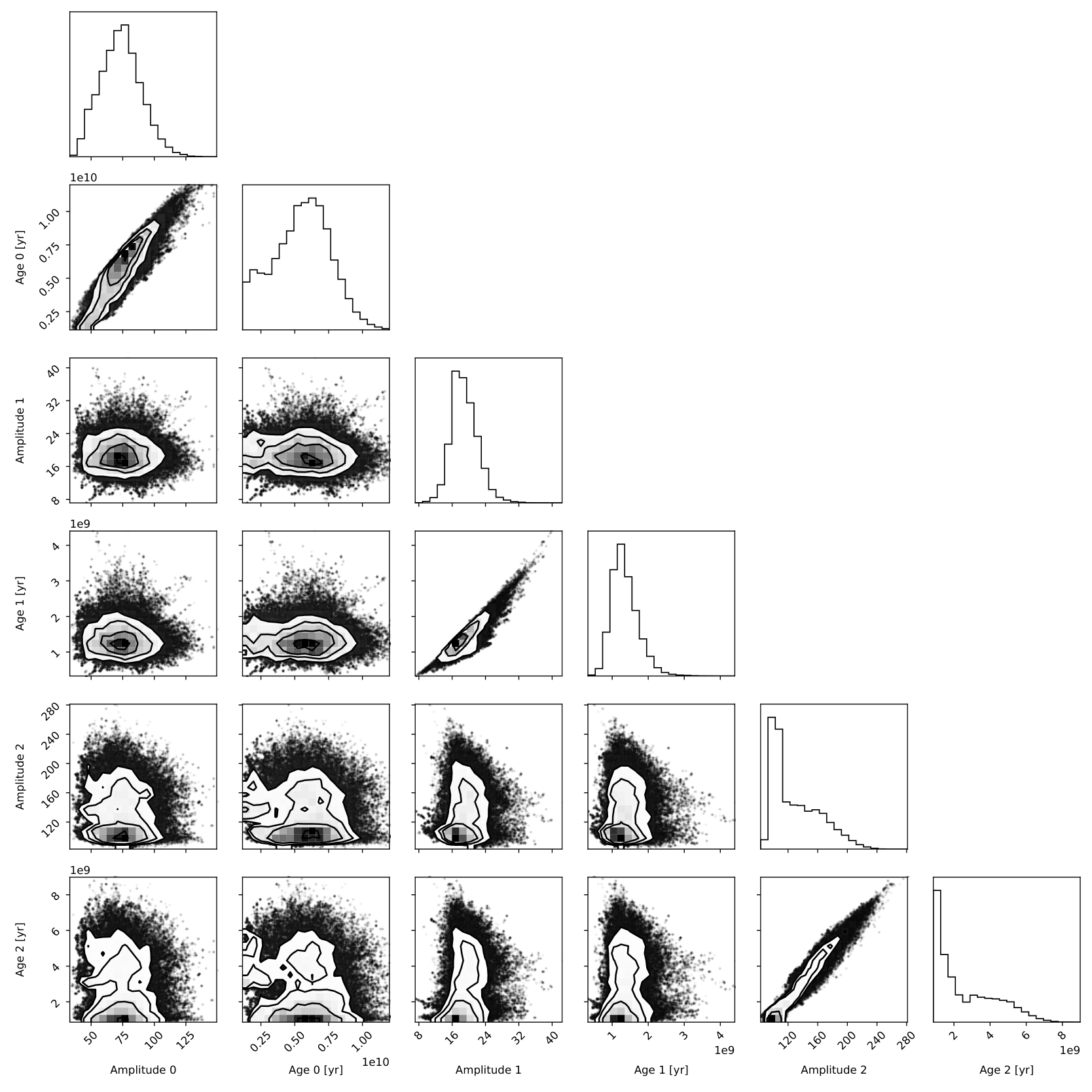
Due to the novelty of our joint-fitting approach, we describe three additional validation steps here. First, we show a typical cornerplot for one of the jointly fitted SEDs (the example shows NSA7167) in Figure 17. We find that the inferred parameters are strongly peaked and unimodal, though there is a degeneracy between the age and amplitude (stellar mass) inferred for each cluster SED. This is a physically expected effect since an increase in the age leads to a drop in the mass-to-light ratio of the stellar population, meaning that more stellar mass is necessary to achieve the same luminosity. We find no significant degeneracy between parameters inferred for different cluster SEDs.
Next, we show in Figure 16 a comparison between the SED fitting results using the global optical photometry and those derived using the cluster SEDs. We find no evidence for a systematic shift between the global and joint fitting methods. Indeed, the total stellar mass and star formation rate inferred via the joint fit method is in good agreement with those estimated via the global fit method, as shown by the text in each panel.
Finally, as stated in the main text, we assume a fixed metallicity in the SED fitting presented in this paper. There is some evidence that low surface brightness galaxies may have higher than average gas-phase metallicities (Greco et al. 2018a; Sánchez Almeida et al. 2018), though we caution that these results contain only three low surface brightness galaxies, and that these low surface brightness galaxies are an optically-selected sample (as opposed to the H I-selected UDGs in the sample discussed in this work). We find that assuming solar metallicity models shifts the total star formation rate and stellar mass estimates by less than 0.1 dex compared to the fiducial estimates. The stellar masses estimated using solar metallicity models are slightly lower (with a median difference between solar metallicity and fiducial values of -0.08 dex), and the star formation rates are slightly higher (with a median difference of 0.09 dex). This shift is expected – the higher metallicity models are redder at fixed age, meaning that the best-fit stellar populations will be on average slightly younger at fixed color.
Appendix C H I Profile Recovery
Although the subset of the Janowiecki et al. 2019 UDGs with resolved H I observations from Gault et al. 2021 are disjoint from the subset of Janowiecki et al. 2019 UDGs in this work, we can do a simple test of our H I profile recovery alone using the Gault et al. 2021 galaxies.
In Figure 18 we show a comparison between the H I profiles estimated from the Gault et al. 2021 structural measurements (dashed curves) with profile estimates analogous to those presented in the main body of this work (solid curve and filled region). We also show the directly measured profiles of Leroy et al. 2008 as solid grey curves in each panel. We find that the profiles are generally well-recovered in the range of probed by the Leroy et al. 2008 sample. We do find that the inferred Gault et al. 2021 profiles with very high H I surface densities (AGC749251, M⊙ pc-2) are significantly underestimated. However, we caution that the Gault et al. 2021 profiles are estimated from their measured H I masses, isophotal sizes, and fraction of H I contained within that isophotal size – not directly measured profiles. We also note that it is expected theoretically that the maximum H I surface density of these systems should be M⊙ pc-2 on kiloparsec scales (Krumholz 2013).
We thus find that our average H I profile estimation technique works well to capture the average behavior of the Gault et al. 2021 resolved UDG measurements, though we caution that this test is quite limited in scope due to the inclusion of the Gault et al. 2021 inferred profiles in creating the profile estimation method. As expected, the average estimation method performs better for galaxies with average H I surface densities than for UDGs with notably high or low H I surface densities. Because our analysis focuses on the bulk behavior of the dwarfs in our sample as opposed to the properties of individual galaxies (and because high resolution H I data are not yet available for sufficiently large samples of UDGs), we find in this limited test case that our estimation method is well-suited for the purpose of this work.