Consistent Selection of the Number of Groups in Panel Models via Cross-Validation
Abstract
Group number selection is a key problem for group panel data modeling. In this work, we develop a cross-validation (CV) method to tackle this problem. Specifically, we split the panel data into two data folds on the time span with a buffer zone, with group structure preserved for individuals. We first estimate the group memberships and parameters on one data fold, then plug in the estimates and utilize the other data fold to evaluate a designed criterion. Subsequently, the group number is estimated by minimizing the average criterion across all data folds. The proposed CV method has two advantages compared to existing approaches. First, the method is totally data-driven; thus no further model-specific tuning parameters are involved. Second, the method can be flexibly applied to a wide range of panel data models. Theoretically, we establish the estimation consistency by taking advantage of the optimization process on the training data fold. Experiments are carried out with a variety of synthetic datasets and panel models to further illustrate the advantages of the proposed method. Lastly, the CV method is employed to analyze the heterogeneous patterns of stock volatilities in the Chinese stock market during the 2008 financial crisis.
Keywords: Cross-validation; Group number estimation; Group panel data model.
1 Introduction
Panel data modeling is an important research area in statistics and econometrics (Arellano 2003; Ke et al. 2015; Ke et al. 2016; Ando and Bai 2017; Hsiao 2022), as it captures information from both temporal and cross-sectional dimensions. A critical problem in panel data modeling is to characterize the individual heterogeneity resulting from distinct backgrounds and individual characteristics (Bai and Li 2014; Ke et al. 2015; Li et al. 2016; Fan et al. 2018; Hong et al. 2023). In this regard, latent group structures have recently received considerable attention (Ke et al. 2015; Su et al. 2019; Gu and Volgushev 2019; Zhu et al. 2023; Mehrabani 2023). The key assumption in group panel data modeling is that the individuals within the same group share the same set of model coefficients (Ke et al. 2015; Su et al. 2016; Fang et al. 2023). With this specification, research has shown that the latent group structure can capture flexible unobserved heterogeneity of panel data while retaining a parsimonious model form and desirable statistical efficiency.
While group panel data models have proved to be useful, their practical performance is significantly contingent on the specification of the group number. If the group number is under-specified, one will end up with an underfitted model with inferior performance. On the other hand, over-specification of the group number may result in an overfitted model with suboptimal estimation efficiency. Consequently, a critical problem for the group panel data models is how to determine the number of groups.
For selecting the number of groups/clusters, two common approaches are widely used. The first involves the utilization of an information criterion (IC) that integrates both model fitness and model complexity. Methods based on IC are extensively utilized in the literature for tuning parameter selection in model selection tasks (Schwarz 1978; Hurvich et al. 1998; Wang et al. 2009; Zhang et al. 2010). For instance, Naik et al. 2007 extended the Akaike information criterion to mixture regression models for selecting the number of mixture components. Li et al. 2016 employed a specific information criterion to determine the number of structural breaks. Hu et al. 2020 proposed a corrected BIC to determine the number of communities in the community detection task. In the analysis of grouped panel models, Lin and Ng 2012 proposed a modified BIC for linear panel models. Bonhomme and Manresa 2015 used a BIC based criterion for grouped fixed-effects models. Liu et al. 2020 designed a PC criterion for panel models with individual fixed effects. Theoretically, the IC based methods can consistently select the true group number under certain conditions. However, to implement the IC based methods, one still needs to specify certain model-specific tuning parameters, whose choice may depend on the specific model and error distribution, making the procedure subjective and potentially unstable. The second one is the hypothesis testing-based method (Tibshirani et al. 2001; Onatski 2009; Choi et al. 2017). This type of method formulates the group number estimation problem into a sequential hypothesis testing procedure (Hardy 1996; Lo et al. 2001; Bickel and Sarkar 2016). In the investigation of panel models with group structures, Lin and Ng 2012 used a test to test the homogeneity of the data. Lu and Su 2017 proposed a residual-based Lagrange multiplier-type test to determine the group number for linear group panel data models. However, the hypothesis testing-based methods are usually restricted to the linear panel models and cannot provide a unified group number estimation framework with general model forms.
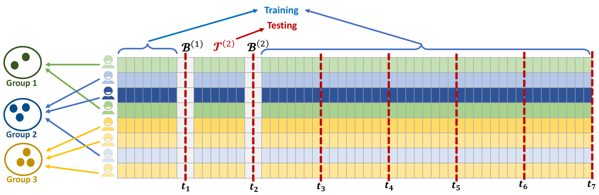
In this work, we propose a unified group number estimation method via cross-validation for general panel data models. The method allows for entirely data-driven implementation, eliminating the need for specifying model-specific tuning parameters. Specifically, we first split the panel data on the time span into two folds, and a time gap is specified between the two data folds as a buffer zone to accommodate temporal dependence. We use the first data fold for model training and the second for model testing, and then swap their roles. This splitting method maintains the group structure of individuals of the panel data; see Figure 1 for illustration. Subsequently, we estimate the group structure and model parameters based on the training data, given a specified group number . Then, we evaluate a designed criterion with the testing data by approximating the loss with a local quadratic function. Finally, the determination of the group number is achieved by minimizing the average criterion over two data folds.

The idea is in spirit similar to the -fold cross-validation (CV) method, which is widely used as a common practice to select tuning parameters (or candidate models) or evaluate the prediction performance of a wide range of machine learning methods (Wang and Leng 2007; Hastie et al. 2009; Wang et al. 2007b). For model selection, the CV method is typically used to select important tuning parameters for machine learning models, which can yield the best prediction accuracy. For example, it can be applied to select the penalty level for the regularized regression models (Tibshirani 1996; Wang et al. 2007a). In model assessment, the CV method is used to quantify the prediction accuracy (Bates et al. 2024) or make valid statistical inferences (Fan and Yim 2004). For example, Fan et al. 2012 proved that a consistent variance estimation can be obtained for ultrahigh dimensional regression model with the CV technique. For the group panel data model, the group number can be treated as a tuning parameter, therefore our task is to utilize the CV method for selecting instead of assessing model predictions.
However, existing theoretical properties have shown that the -fold CV method tends to select an overfitting model when applied to model selection tasks (Shao 1993; Wang et al. 2007b). Nevertheless, we find that it is not true with our task. Notably, the estimation consistency of group number can be established under our scenario. This is mainly because we consider a two-dimensional panel data setting and we conduct the data splitting on the time span. As shown by Figure 1, the splitting on the time span allows us to preserve the group structure on all data folds, and this is the key to establishing the selection consistency by connecting to the optimization procedure with the training data fold. A similar procedure has been adopted by Zou et al. 2020 to select the number of change points in the change point detection area. We also refer to Wang 2010; Chen and Lei 2018; Lei 2020; Rabinowicz and Rosset 2022 for the relevant literature using CV methods for model selection and relevant inference tasks. However, to the best of our knowledge, the CV method has not been introduced to group number estimation in the group panel models.
In particular, our method can be applied to a wide range of panel models, including linear panel models (Lin and Ng 2012) and nonlinear panel models, such as probit panel model (Su et al. 2016), logit panel model (Liu et al. 2020), as long as the corresponding loss function can be approximated with a local quadratic function form (Wang and Leng 2007; Zou et al. 2020; Zhu et al. 2021). Consequently, it provides a flexible and unified parametric solution for selecting the group number in group panel data models. Our theoretical framework establishes the connection between the estimation consistency and the optimization procedures (Lin and Ng 2012; Bonhomme and Manresa 2015; Liu et al. 2020). We further evaluate the validity of the CV method when applied to a linear panel model with nonstationary covariates (Phillips and Moon 1999; Tu and Yi 2017), and a classical interactive effects model (Bai 2009; Miao et al. 2020) in Appendix . Numerical evidence suggests that the CV method can still yield satisfactory performance with minor adaptations, illustrating a considerable potential for extensions of the proposed CV method.
The rest of the article is organized as follows. In Section 2, we provide a selection criterion for group number estimation, offering a detailed exposition of the procedure employed for the estimation. Theoretical properties on asymptotic selection consistency are established in Section 3. Subsequently, Section 4 extends the proposed selection criterion to group panel models with fixed effects. Numerical studies are presented in Section 5 and an empirical study of stock volatilities in Chinese stock market during the 2008 financial crisis is presented in Section 6. Finally, we conclude the article with a discussion in Section 7. Additional numerical studies, model extensions, proofs, and technical lemmas can be found in the Appendices –.
2 Selection with Cross-Validation
2.1 Model and Notation
Let be the response variable and be the associated -dimensional covariate vector collected from the th () individual at the th () time point. The panel data are denoted as with . Suppose that the individuals are divided into groups, where individuals in the th group () share the same regression coefficient vector . For each individual , denote as its true group membership. Let collect the indices of individuals in the th group, and denote as the corresponding partition over . More generally, for any given integer , we denote as a partition of , where collects the indices of individuals assigned to the th group. The associated group-specific coefficient vectors are denoted as . For each individual , we write for its group membership under partition , therefore equivalently . In practice, the true group number , partition , and group parameters are all unknown and need to be estimated. To be more specific, given a pre-specified group number , we estimate the unknown memberships and group parameters by minimizing the following loss function :
| (2.1) |
where represents the loss function evaluated at with parameter , and . The optimization in (2.1) can be solved via a -means type algorithm (Liu et al. 2020), summarized in Algorithm 1.
To estimate the unknown group number , a popular way is to adopt the IC methods. However, such methods still rely on a tuning constant in the penalty term that must be pre-specified (Su et al. 2016; Liu et al. 2020). The choice of this constant may depend on model and error specifications, leading to instability in practice. Thus, we aim to develop a data-driven procedure to estimate .
General Notation. For a positive integer , denote . We use to denote the Euclidean norm of a vector. For any matrix , denotes the Frobenius norm of . In addition, for any symmetric matrix , let and denote the maximum and minimum eigenvalues of , respectively. Moreover, for any vector , let denote its th element and define for any positive definite matrix . Similarly, for any two vectors , define for any positive definite matrix and . For any twice-differentiable function with respect to a vector , we use and to denote its first and second order derivatives, respectively. For a sequence of positive real numbers and a sequence of random variables , we denote if there exists a constant such that holds for large enough with probability tending to one.
2.2 Quadratic Approximation to Objective Function
To estimate the number of groups in a data-driven manner, we need to construct a selection criterion with the cross-validation (CV) method. Following a common practice in the literature (Yao 1988; Zou et al. 2020; Zhu et al. 2021), the selection criterion is designed based on a quadratic approximation to the loss function . To motivate the idea, we first define the node-wise loss function as
| (2.2) |
Subsequently, we could obtain a node-wise estimator by minimizing as . Then we can approximate by using a Taylor expansion in the neighborhood of as
where the first term is not related to . Define and . We note that , then we have
| (2.3) |
For convenience, we consider the following quadratic approximation to the loss function in (2.1) as
| (2.4) |
by ignoring the constants. We remark that the quadratic approximation in (2.4) is valid provided the loss function possesses continuous second-order derivatives, which is satisfied by many commonly used models such as the linear panel model, probit panel model, and Poisson panel model.
2.3 Selection Criterion with Cross-Validation
Based on the quadratic approximation (2.4), we propose a selection criterion using 2-fold cross-validation. With this partition, we split the data into two folds and on the time span, as illustrated in Figure 1. To ensure that the dependence between the two data folds is negligible, a buffer zone with time length is specified between the two folds, i.e., and . Such buffering (or gap) strategies have been widely adopted in cross-validation and sample-splitting procedures for dependent data (Racine 2000; Bergmeir et al. 2018; Semenova et al. 2023). Our theoretical analysis suggests that should satisfy to guarantee that the dependence between the two data folds is asymptotically negligible under the -mixing condition. In practice, we recommend using with , which yields satisfactory numerical performance.
To conduct the CV method, we first estimate the parameters and the group memberships using each data fold separately as
Then we evaluate the out-of-sample loss on the other data fold, respectively as and . Subsequently, we select by minimizing the following CV based criterion,
| (2.5) |
where denotes the maximum number of groups under consideration. The selection procedure is summarized in Algorithm 2. We remark that one can also consider a -fold CV procedure for estimating to retain more training data, and the implementation is presented as follows.
Remark 1.
(-fold CV Implementation) First, we segment the time span into consecutive folds of approximately equal length, where the time points in the th fold are collected in the set . Suppose that the data folds are segmented by the time points , where for and . Then we specify the th buffer zone as and we set for convenience. Subsequently, we evaluate the -criterion for rounds. For the th round, we take as the time span in the testing data fold, and as the training data fold. The above process is illustrated in Figure 2. Lastly, the group number is estimated by , where is the testing data fold in the th round, and denotes the estimates obtained using the corresponding training fold.
We explain the rationale of (2.5) by decomposing . Specifically, we first define and with any given . Let () denote the estimated group structure using . We can then decompose as
| (2.6) |
with the notation and for , . The third term is a cross term which is dominated by the first two terms under both underfitting and overfitting cases. In the underfitting case (i.e., ), will dominate with a large prediction error on the testing dataset. In the overfitting case (i.e., ), we can show that will dominate by taking consideration of the optimization procedure on the training data fold. Consequently, plays a role similar to the penalty term in the BIC or AIC selection, while using a data-driven strategy. This avoids setting a user-determined constant in information criteria.
Remark 2.
We consider a simple univariate model for illustration, i.e., where is the independent noise term with mean 0 and variance . For estimation, we use the least squares objective function, i.e., . Suppose the group structure is estimated using the first fold as for . Then we have and . In this case, we have and . This yields
| (2.7) |
and in this case since . The form is similar to the IC based method for determining the group number (Bonhomme and Manresa 2015; Su et al. 2016; Liu et al. 2020). The first term in (2.7) is used to evaluate the goodness-of-fit level, and the second term plays the role of penalty for model complexity as in the IC method. In contrast to the user-specified tuning parameter typically involved in the second penalty term for the IC method, the amount of “penalty” in (2.7) can be totally determined by the data information. As a consequence, our data-splitting method is tuning-free and thus more user-friendly.
2.4 Comparison with Existing Methods
In this section, we compare the proposed CV method with the widely used information criterion (IC) and hypothesis testing (HT) methods in detail. In addition, we also compare with the CV method for the change points’ number estimation problem to clarify the differences.
2.4.1 Comparison with IC and HT Methods
We first compare the proposed CV based estimation with two widely used methods for estimating in the group panel data literature. The first is the IC based methods (Bonhomme and Manresa 2015; Su et al. 2016; Liu et al. 2020), and the second is the hypothesis testing-based method (Lu and Su 2017). The IC based methods minimize the criterion in the following form, i.e.,
| (2.8) |
where is the penalty function with model-specific tuning parameter . Particularly, for different panel data models, different functions are utilized. For the linear panel data model, Bonhomme and Manresa 2015 used a BIC based criterion and set , where is an estimated variance by setting as a sufficiently large value. However, they did not provide the theoretical analysis for estimating . Subsequently, Su et al. 2016 and Liu et al. 2020 studied more generalized panel data models but they set different penalty forms for different models. To be more specific, Su et al. 2016 recommended using with for the linear model, and for the probit model. In contrast, Liu et al. 2020 set with for the linear model, and for the probit model. We summarize different penalty functions in the IC methods in Table 1. In addition to the IC methods, the hypothesis testing method was studied by Lu and Su 2017 for the linear panel data model. They considered the testing problem as
and they derived a residual-based LM-type test statistic. However, their test statistic can only be applied to linear models.
| Model | |||
|---|---|---|---|
| Bonhomme and Manresa 2015 | Linear | – | |
| Su et al. 2016 | Linear | ||
| Probit | |||
| Liu et al. 2020 | Linear | ||
| Probit |
In summary, compared with these existing methods, we highlight the merits of our CV based method as follows. First, we provide a unified group number selection method, which can be flexibly applied to various panel data models. In contrast, the IC based method requires specifying the penalty function (2.8) individually for each panel data model, while the hypothesis testing method needs to derive valid testing rules case by case. Actually, as shown by our simulation study, we find that our CV method can work well under various panel models, while the IC methods (Su et al. 2016; Liu et al. 2020) generally yield larger estimation errors when applied beyond the specific models for which their penalties were tuned. Second, the proposed CV method is model-specific tuning free, namely, it does not need to select extra tuning parameters () as the IC methods. The selection of can be subjective and may not be adaptive to various datasets. Third, our numerical studies show that the CV method achieves better performance under weak signals (i.e., when the group differences are small), demonstrating its robustness.
2.4.2 Comparison with the CV Method in Change Points Number Estimation
The proposed method shares great similarity with the CV method designed by Zou et al. 2020 for estimating the number of change points. They consider a similar quadratic loss function for estimating the number of change points. Despite the similarity, we would like to highlight two differences between the proposed methodology with their approach. First, the data structure is different for the change point detection problem and panel data modeling. To be more specific, Zou et al. 2020 considered a one dimensional problem, i.e., , and aimed to estimate the change points along . They split the time points into odd- and even-indexed subsets to preserve the time dynamic patterns on each data fold when conducting the CV method. On the other hand, the panel data contains two dimensions: the individuals () and the time span (). This leads to different definitions of “groups” under the above two settings. In the change points detection problem, groups are defined over the time span to be segmentations of . In contrast, in the panel data setting, groups refer to partitions of individuals . For the group panel data model, we typically use a -means type algorithm to partition among the individuals, while for change point detection, the binary segmentation and optimal partitioning algorithms are utilized for identifying the segmentations along the time span.
Second, in the panel data setting, determining how to partition the dataset is crucial, given its two-dimensional structure. The first splitting scheme is to split the dataset on the individual dimension, which is referred to as individual-based splitting. In this way, the time dynamics pattern can be preserved on each data fold. The second is to split on the time dimension, which is referred to as temporal-based splitting. In this way, the group structure of all individuals can be preserved. For comparison, we conduct the CV methods for both schemes with a simple simulation example, where the details are stated in Appendix and we include Figure 3 here for illustration.
It shows that the -criterion (2.4) tends to monotonically decrease as increases for the individual-based splitting scheme, while it exhibits an elbow point at for the temporal-based splitting scheme. This implies the temporal-based splitting scheme (adopted in our framework) is the appropriate choice. We further discuss the intuitions behind this phenomenon in Remark 3.
3 Theoretical Properties
3.1 Technical Conditions
We first introduce multi-index notation to handle higher-order partial derivatives in a unified manner. For and a multi-index with non-negative integer entries, denote and define the th order partial derivative
To establish the theoretical properties, the following conditions are required.
- (C1)
(Parameter Space) Suppose there exists a constant such that
- (C2)
(Distribution) The observations satisfy the following dependence structure.
- (C2.1)
(Time Dependence) For each , the process is stationary and -mixing with mixing coefficients . Moreover, satisfies for all and some positive constants and .
- (C2.2)
(Individual Independence) are independent across .
- (C2.1)
- (C3)
(Buffer Length) The length of the buffer zone between the two folds satisfies , , and as .
- (C4)
(Smoothness) There exists a non-negative function such that, for all with and , and for every multi-index with ,
(3.1) and . The function satisfies the exponential tail condition
(3.2) for some constants and . Furthermore, there exists a function with such that for every multi-index with and every with .
- (C5)
(Bounded Moments) There exist a non-negative function and two integers , with and such that, for every multi-index with and every with , the following holds almost surely,
(3.3) - (C6)
(Convexity) For each , define for . There exist positive constants and such that .
- (C7)
(Identification) Let . The following identification condition holds: for every ,
The same condition also holds for , where .
- (C8)
(Sample Size) Let with . Suppose and for some , with .
- (C9)
(Group Size) For all , there exists a positive constant such that as .
- (C10)
(Group Separation) Let .
We explain the rationale of the technical conditions in detail as follows. First, Condition (C1) assumes that the parameter space is compact, which is a regular condition in literature (Bonhomme and Manresa 2015; Su et al. 2016; Liu et al. 2020). Condition (C2) specifies the dependence structure of the observations. Specifically, (C2.1) assumes that for each individual, weak time dependence is allowed across the time dimension, which is milder than the i.i.d. condition in Zou et al. 2020. (C2.2) assumes cross-sectional independence, i.e., the individuals are mutually independent. This dependence assumption is widely specified in the panel data literature (Gao 2007; Bonhomme and Manresa 2015; Sarafidis and Weber 2015; Liu et al. 2020). Condition (C3) regulates the length of the buffer zone introduced in our cross-validation scheme to mitigate the temporal dependence between the two data folds (Semenova et al. 2023). Condition (C4) assumes a certain extent of smoothness for the loss function as well as its derivatives. In addition, the exponential bound is imposed on the tail probability of the related function, and similar conditions are assumed by Bonhomme and Manresa 2015 and Liu et al. 2020. Condition (C5) basically requires a bounded moment condition for the th moment of the derivatives, which is also assumed in the relevant literature to ensure the grouping accuracy (Hahn and Newey 2004; Su et al. 2016; Liu et al. 2020).
Next, Condition (C6) assumes convexity within the interested area, and Condition (C7) is an identification condition imposed on each individual to ensure the local minimum at the true value. Condition (C8) allows to grow exponentially fast as . As a consequence, it is suitable for panel data with large and moderately large . We remark that this condition is milder than the assumption imposed in several existing methods (Hahn and Newey 2004; Su et al. 2016), which require should not grow polynomially fast with . In addition, we remark that we require to extract the major term under the overfitting scenario, which is further shown to be lower bounded in Theorem 2. Condition (C9) assumes that the group size should diverge at the same rate as the total number of individuals . Lastly, Condition (C10) imposes a sufficiently large gap between the true group coefficients, which is necessary for group membership estimation. By Conditions (C1)–(C10), we can obtain the group estimation consistency result when (Liu et al. 2020, Theorem 2). Specifically, for each estimated group , the group estimation consistency implies that there exists a true group such that .
3.2 Selection Consistency
Recall that is the true group partition with , and we treat as fixed memberships without randomness. Similarly, is the estimated group partition using when groups are specified, where . In the following we aim to prove the estimation consistency of the group number using the proposed CV estimation procedure. It suffices to show that holds with probability tending to one under both the underfitting case (i.e., ) and the overfitting case (i.e., ). For the underfitting part, the proof basically relies on the group difference condition (C10). We show that there exists at least one group that is sufficiently distant from the others, leading to a large value when .
However, the proof for the overfitting part is more challenging and we illustrate the basic idea as follows. Through a careful decomposition of in our theoretical analysis, we extract the leading term as
| (3.4) |
The establishment of the above result relies on our condition in (C8). This interesting observation links the prediction loss on with the training loss reduction using . Similar results are also established by Zou et al. 2020 when estimating the number of change points with CV method, but we rely on different techniques to show this result. As long as , the estimation consistency can be proved. We formally state this result in the following Theorem 1.
Theorem 1.
The proof of Theorem 1 is provided in Appendix . It implies that the estimation consistency can be obtained as long as the -criterion continues to decrease sufficiently as increases on the training data fold. We then aim to establish the above critical lower bound condition (3.5). First, under the assumed conditions, we show that difference can be sufficiently approximated by the loss difference, i.e., . This approximation error is negligible with certain estimation precision for (see Lemma for details). We note that is minimized by exhausting all -partitions of , thus it should be smaller than the optimal partition that partitions further into groups. We denote the corresponding loss function by . This allows us to lower bound the left side of (3.5) by . With this insight, we establish the lower bound in the following theorem.
The proof of Theorem 2 is provided in Appendix . We explain the rationale as follows. As we comment before, the lower bound condition (3.5) is further reduced to investigating the optimal partition of the true groups. To illustrate our basic idea, we consider the case when is increased from to , and thus there exists one true group partitioned into and . Define
It can be shown that can be approximated by
| (3.6) |
where is the estimates obtained with individuals in for , and . Further analysis shows that (3.6) can be simplified as with
| (3.7) |
where , and for . As a result, it aims to find a partition which maximizes the square of differences of two sample means, i.e., and . We visualize this procedure in Figure 4 for illustration. Note that as , we should have asymptotically converges to a normal distribution. This simplification allows us to derive the lower bound for ; see Lemma for details.

Lastly, we comment on the possible gap between and the minimum attained by the algorithm. To minimize the loss function, we typically utilize a -means type algorithm for model estimation; see Algorithm 1. Usually, a global optimum cannot be guaranteed by the -means algorithm, but a local minimum can be assured. To partially avoid this issue, we follow Liu et al. 2020 to specify multiple initial values to ensure a good convergence, and it yields satisfactory numerical performance in our simulation studies. According to our theoretical analysis, the conclusion in Theorem 2 still holds if the minimum achieved by the algorithm stays not too distant from . We present the requirement in the following corollary.
Corollary 1.
Remark 3.
The above theoretical analysis explains the rationale of our data splitting mechanism on the time span in Figure 1. Particularly, since the two data folds share the same group structure , we can successfully link the dominating term (3.4) to the optimization on the training data fold . We further connect this optimization to the maximization of (3.7) with respect to to establish the lower bound. This is the key ingredient for analyzing the overfitting case. On the other hand, if we split the panel data on the individuals (denoted as and ), we need to re-estimate the memberships on with obtained from . Therefore, it does not involve an optimization procedure to seek the best partition for the individuals on the testing data fold. A similar phenomenon is also observed for estimating the clustering number of clustering tasks, which is known as the “double dipping” problem in the clustering literature (Chen and Witten 2023; Yun and Foygel Barber 2023; Gao et al. 2024). We also compare our theoretical frameworks with the CV method used in change point detection of Zou et al. 2020, and we refer to Remark in Appendix for details.
4 Group Panel Data Model with Fixed Effects
4.1 Panel Data Estimation with Fixed Effects
In this section, we further discuss group number estimation based on the cross-validation method for nonlinear panel data models with fixed effects. In practice, individual-level heterogeneity may exist, and the cross-validation method needs to be revised to accommodate the individual-specific heterogeneity. Suppose the fixed effect of individual is denoted by , which characterizes individual-level heterogeneity. With a slight abuse of notation, throughout this section, we use and to denote the per-observation loss and the total loss when the individual fixed effects are present. We can obtain parameter estimation by minimizing the loss function with a pre-specified group number , i.e.,
| (4.1) |
where and represents the loss function on with parameters and . Here we treat as fixed effects in our analysis, which is also used in panel data literature (Bonhomme and Manresa 2015; Liu et al. 2020). In practice, we can use a profile objective function for estimation. Specifically, define and then the profile objective function is given by
| (4.2) |
A feasible iterative algorithm for obtaining is summarized in Algorithm 3. Subsequently, we discuss the estimation of in the presence of the fixed effects based on the profile objective function. We define , and . Similarly, define and and let and . Following the literature (Liu et al. 2020), denote
| (4.3) | ||||
Denote . In addition, define and , , , , in the same way at the true value. Specifically, we use to denote and use to denote . Similarly, define , , , , , in the same way at the true value. Given the group memberships , we can define and verify that
To derive a simple yet effective loss function when the fixed effects are present, we need the following result on estimation properties. The technical conditions are listed in Appendix .
Proposition 1.
The proof of Proposition 1 is given in Appendix . First, the leading term involves both and . Particularly, the term is an extra bias term caused by the individual-level fixed effects, which is in the order of . It cannot be reduced by using aggregated information of all individuals. The bias term will disappear when the fixed effects are not present. Second, as suggested by the expansion of , an individual weighting matrix is involved in the linear leading term . The weighting matrix varies across due to the existence of the fixed effects. Motivated by this fact, we consider a revised weighted quadratic objective function as
| (4.6) |
The -function in (4.6) is actually a reweighted loss function after adjusting to the individual-level heterogeneous weighting matrix . Based on this -function, we obtain the final estimators by .
4.2 Group Number Estimation using Cross-Validation Method
Based on the objective function , we apply the same data-splitting scheme to estimate the number of groups. Specifically, the estimated is given by
| (4.7) |
where , are estimators obtained by applying Algorithm 4 on two data folds respectively. The selection procedure is summarized in Algorithm 5. In what follows, we establish the estimation consistency of under a pivotal condition (i.e., (4.8)) in Theorem 3 and verify the condition in Theorem 4.
Theorem 3.
The proof of Theorem 3 is provided in Appendix . The condition (4.8) means that the reduction in the -function due to further partitioning by (with ) should also be at least equal to the rate , which is the same as (3.5). In the following, we show that the lower bound condition (4.8) can be satisfied by using the revised -function.
Theorem 4.
The proof of Theorem 4 is provided in Appendix . The conclusion of Theorem 4 ensures that (4.8) holds automatically. As an immediate consequence of Theorem 3, we can conclude that still holds for the group panel data model with fixed effects. Following the similar routine of the overfitting part in Theorem 2, we show that the lower bound in (4.8) can be guaranteed by the optimization procedure. We also refer to Appendix for two possible extensions of our proposed method.
5 Numerical Studies
5.1 Simulation Models and Selection Criteria
To evaluate the finite sample performance of the CV method, we conduct a number of simulation studies in this section. For comparison, we include several competing methods discussed in Section 2.4.1. We refer to the information criteria given by Bonhomme and Manresa 2015, Su et al. 2016 and Liu et al. 2020 as BIC, LIC (Lasso-based information criterion) and PC (penalty criterion), respectively in the following. In addition to the IC based methods, we also consider the method based on hypothesis testing (denoted as HT) proposed by Lu and Su 2017. Since the HT method is designed only for linear models, we include it only for DGP 1 and DGP 2.
We consider four data generating processes (DGPs), including linear static (DGP 1) and dynamic panel models (DGP 2), a dynamic probit panel model (DGP 3), and a static Poisson panel model (DGP 4). The sample sizes are set to and . The true number of groups is , with equal group sizes . The detailed specifications of the four DGPs (i.e., DGP 1–DGP 4) are deferred to Appendix due to space limitations.
5.2 Simulation Results
The random experiments are repeated for times. To measure the finite sample performance, we report the accuracy as Acc, the mean estimation bias as Bias and the root mean squared error as RMSE, where denotes the estimated group number in the th replicate. The numerical results for all four DGPs are summarized in Table 2. For visualization, the distribution of under DGP 2 (dynamic linear panel model with fixed effect ), DGP 3 (dynamic probit panel model), and DGP 4 (static Poisson panel model) is presented in Figure 5, while the corresponding plots for DGP 1 (static linear panel model with and without fixed effects) and DGP 2 (dynamic linear panel model without fixed effects) are deferred to Appendix due to space limitations.
First, the estimation accuracy of the CV method improves substantially as and increase. To further illustrate the consistency property established in Theorems 1 and 3, we report the selection accuracy of CV over a wider range of combinations in Figure in Appendix , where the accuracy approaches as and grow large. Besides, the proposed CV method performs better than, or is at least comparable to, the competing methods across the considered DGPs. The BIC, PC, and LIC methods severely underestimate with accuracies essentially equal to zero. The HT method becomes comparable to CV only for linear panel models with sufficiently large , but is inferior to CV when is small or moderate, and is not applicable to the nonlinear models as in DGP 3 and DGP 4. Particularly, the advantage of the proposed CV method is more pronounced for the Poisson panel model (in DGP 4). This implies that the IC methods are sensitive to tuning parameter specifications and requires appropriate tuning to deliver a good performance. In contrast, our CV method does not involve this tuning process and can deliver a more robust performance with various panel models.
| Method | DGP 1. | DGP 1. (with ) | DGP 2. | DGP 2. (with ) | DGP 3 | DGP 4 | ||||||||||||||
|---|---|---|---|---|---|---|---|---|---|---|---|---|---|---|---|---|---|---|---|---|
| Acc | Bias | RMSE | Acc | Bias | RMSE | Acc | Bias | RMSE | Acc | Bias | RMSE | Acc | Bias | RMSE | Acc | Bias | RMSE | |||
| 80 | 80 | BIC | 0.00 | -2.95 | 2.95 | 0.00 | -2.99 | 2.99 | 0.00 | -3.00 | 3.00 | 0.00 | -3.00 | 3.00 | 0.00 | -2.05 | 2.06 | 0.00 | -2.00 | 2.00 |
| PC | 0.00 | -3.00 | 3.00 | 0.00 | -3.00 | 3.00 | 0.00 | -3.00 | 3.00 | 0.00 | -3.00 | 3.00 | 0.00 | -3.00 | 3.00 | 0.00 | -3.00 | 3.00 | ||
| LIC | 0.00 | -1.62 | 1.69 | 0.00 | -1.75 | 1.80 | 0.00 | -2.00 | 2.00 | 0.00 | -2.00 | 2.00 | 0.00 | -3.00 | 3.00 | 0.00 | -3.00 | 3.00 | ||
| HT | 0.00 | -1.03 | 1.07 | 0.00 | -1.03 | 1.07 | 0.00 | -1.39 | 1.47 | 0.00 | -1.39 | 1.47 | - | - | - | - | - | - | ||
| CV | 0.07 | -1.23 | 1.42 | 0.08 | -1.16 | 1.41 | 0.02 | -1.66 | 1.75 | 0.03 | -1.61 | 1.72 | 0.02 | -2.27 | 2.43 | 0.23 | -0.68 | 1.11 | ||
| 120 | BIC | 0.00 | -2.98 | 2.99 | 0.00 | -3.00 | 3.00 | 0.00 | -3.00 | 3.00 | 0.00 | -3.00 | 3.00 | 0.00 | -2.06 | 2.07 | 0.00 | -2.00 | 2.00 | |
| PC | 0.00 | -3.00 | 3.00 | 0.00 | -3.00 | 3.00 | 0.00 | -3.00 | 3.00 | 0.00 | -3.00 | 3.00 | 0.00 | -3.00 | 3.00 | 0.00 | -3.00 | 3.00 | ||
| LIC | 0.00 | -1.37 | 1.45 | 0.00 | -1.48 | 1.56 | 0.00 | -2.00 | 2.00 | 0.00 | -2.00 | 2.00 | 0.00 | -3.00 | 3.00 | 0.00 | -3.00 | 3.00 | ||
| HT | 0.12 | -0.87 | 0.95 | 0.11 | -0.88 | 0.95 | 0.02 | -1.02 | 1.04 | 0.01 | -1.02 | 1.04 | - | - | - | - | - | - | ||
| CV | 0.26 | -0.65 | 1.09 | 0.28 | -0.59 | 1.04 | 0.10 | -1.13 | 1.32 | 0.10 | -1.14 | 1.31 | 0.10 | -1.56 | 1.78 | 0.69 | 0.10 | 0.71 | ||
| 160 | BIC | 0.00 | -3.00 | 3.00 | 0.00 | -3.00 | 3.00 | 0.00 | -3.00 | 3.00 | 0.00 | -3.00 | 3.00 | 0.00 | -2.08 | 2.09 | 0.00 | -2.00 | 2.00 | |
| PC | 0.00 | -3.00 | 3.00 | 0.00 | -3.00 | 3.00 | 0.00 | -3.00 | 3.00 | 0.00 | -3.00 | 3.00 | 0.00 | -3.00 | 3.00 | 0.00 | -3.00 | 3.00 | ||
| LIC | 0.00 | -1.17 | 1.23 | 0.00 | -1.24 | 1.31 | 0.00 | -2.00 | 2.00 | 0.00 | -2.00 | 2.00 | 0.00 | -3.00 | 3.00 | 0.00 | -3.00 | 3.00 | ||
| HT | 0.44 | -0.55 | 0.77 | 0.42 | -0.56 | 0.78 | 0.11 | -0.89 | 0.94 | 0.10 | -0.90 | 0.95 | - | - | - | - | - | - | ||
| CV | 0.59 | -0.20 | 0.76 | 0.57 | -0.13 | 0.81 | 0.22 | -0.74 | 1.07 | 0.25 | -0.72 | 1.05 | 0.34 | -0.82 | 1.23 | 0.91 | 0.07 | 0.38 | ||
| 120 | 80 | BIC | 0.00 | -2.06 | 2.08 | 0.00 | -2.22 | 2.26 | 0.00 | -2.94 | 2.95 | 0.00 | -2.98 | 2.99 | 0.00 | -2.01 | 2.01 | 0.00 | -1.99 | 1.99 |
| PC | 0.00 | -3.00 | 3.00 | 0.00 | -3.00 | 3.00 | 0.00 | -3.00 | 3.00 | 0.00 | -3.00 | 3.00 | 0.00 | -3.00 | 3.00 | 0.00 | -3.00 | 3.00 | ||
| LIC | 0.00 | -1.20 | 1.27 | 0.00 | -1.36 | 1.45 | 0.00 | -2.00 | 2.00 | 0.00 | -2.00 | 2.00 | 0.00 | -3.00 | 3.00 | 0.00 | -3.00 | 3.00 | ||
| HT | 0.02 | -0.98 | 1.00 | 0.01 | -0.99 | 1.00 | 0.00 | -1.10 | 1.14 | 0.00 | -1.11 | 1.16 | - | - | - | - | - | - | ||
| CV | 0.06 | -1.19 | 1.34 | 0.06 | -1.17 | 1.34 | 0.02 | -1.65 | 1.74 | 0.02 | -1.60 | 1.69 | 0.06 | -2.27 | 2.48 | 0.38 | -0.46 | 0.93 | ||
| 120 | BIC | 0.00 | -2.17 | 2.21 | 0.00 | -2.36 | 2.40 | 0.00 | -2.99 | 2.99 | 0.00 | -3.00 | 3.00 | 0.00 | -2.00 | 2.00 | 0.00 | -1.99 | 2.00 | |
| PC | 0.00 | -3.00 | 3.00 | 0.00 | -3.00 | 3.00 | 0.00 | -3.00 | 3.00 | 0.00 | -3.00 | 3.00 | 0.00 | -3.00 | 3.00 | 0.00 | -3.00 | 3.00 | ||
| LIC | 0.00 | -1.06 | 1.09 | 0.00 | -1.11 | 1.15 | 0.00 | -1.99 | 1.99 | 0.00 | -2.00 | 2.00 | 0.00 | -3.00 | 3.00 | 0.00 | -3.00 | 3.00 | ||
| HT | 0.24 | -0.76 | 0.87 | 0.21 | -0.78 | 0.90 | 0.05 | -0.95 | 0.98 | 0.04 | -0.96 | 0.98 | - | - | - | - | - | - | ||
| CV | 0.41 | -0.53 | 0.90 | 0.42 | -0.50 | 0.88 | 0.08 | -1.10 | 1.26 | 0.08 | -1.09 | 1.25 | 0.15 | -1.43 | 1.71 | 0.87 | 0.09 | 0.48 | ||
| 160 | BIC | 0.00 | -2.25 | 2.30 | 0.00 | -2.40 | 2.45 | 0.00 | -3.00 | 3.00 | 0.00 | -3.00 | 3.00 | 0.00 | -2.00 | 2.00 | 0.00 | -2.00 | 2.00 | |
| PC | 0.00 | -3.00 | 3.00 | 0.00 | -3.00 | 3.00 | 0.00 | -3.00 | 3.00 | 0.00 | -3.00 | 3.00 | 0.00 | -3.00 | 3.00 | 0.00 | -3.00 | 3.00 | ||
| LIC | 0.00 | -1.00 | 1.01 | 0.00 | -1.01 | 1.01 | 0.00 | -1.97 | 1.98 | 0.00 | -1.98 | 1.98 | 0.00 | -3.00 | 3.00 | 0.00 | -3.00 | 3.00 | ||
| HT | 0.73 | -0.21 | 0.62 | 0.71 | -0.20 | 0.68 | 0.27 | -0.73 | 0.86 | 0.24 | -0.76 | 0.87 | - | - | - | - | - | - | ||
| CV | 0.73 | -0.11 | 0.56 | 0.73 | -0.07 | 0.57 | 0.30 | -0.68 | 0.95 | 0.31 | -0.61 | 0.91 | 0.47 | -0.59 | 1.00 | 0.93 | 0.08 | 0.37 | ||
6 Empirical Study
In this section, we apply the proposed method to the Chinese A-share market dataset collected from CSMAR (https://data.csmar.com/). Our study aims to investigate the heterogeneous group patterns in the Chinese stock market from July 1, 2006 to November 30, 2009 including the financial crisis in 2008, providing insights into market structure dynamics and systemic risk assessment. To demonstrate the robustness of the proposed method, we also apply the CV method to a variety of synthetic datasets with extensive simulation studies; see Appendix for details.
6.1 Data Description
The empirical analysis employs data from the Chinese A-share market extracted from the CSMAR database. Our sample consists of 80 firms from the finance, properties, and commercial sectors that were continuously listed on either the Shanghai Stock Exchange or Shenzhen Stock Exchange from July 1, 2006 to November 30, 2009.
The dependent variable is the daily volatility, measured by the daily absolute return for company on the th trading day where is the adjusted closing price of company on the th trading day. This measure of volatility is widely used in the literature as it captures the magnitude of daily price movements while being robust to the direction of price changes (Ding et al. 1993; Corsi 2009). For the covariates, we employ a set of market microstructure indicators, i.e., the previous trading day’s price range (defined as the difference between daily high and low prices), logarithmic trading volume (Xu et al. 2006), logarithmic turnover ratio (Barinov 2014), and logarithmic closing price.
To investigate the structural changes in market behavior during the 2008 financial crisis, we follow Ando and Bai 2017 to partition the sample period into five distinct phases as
- •
Period 1 (Pre-crisis): July 1, 2006 to December 31, 2006
- •
Period 2 (Crisis onset): July 1, 2007 to December 31, 2007
- •
Period 3 (Crisis peak): February 1, 2008 to August 31, 2008
- •
Period 4 (Crisis aftermath): October 1, 2008 to March 31, 2009
- •
Period 5 (Recovery): May 1, 2009 to November 30, 2009.
To better understand the intrinsic data patterns within each period, we visualize cross-sectional correlation matrices of across 80 firms for each period in Figure 6. It shows that the stocks exhibit stronger correlations during the crisis periods 3 and 4.

6.2 Estimation Results
Subsequently, we model the volatility using two linear panel models. First, we consider a linear panel model without fixed effects:
| (6.1) |
where is an idiosyncratic error term. The autoregressive term captures volatility persistence, while the group-specific slope allows the sensitivities to market microstructure indicators. Second, to account for unobserved time-invariant individual heterogeneity, we extend the model by incorporating individual fixed effects:
| (6.2) |
where denotes the firm-specific fixed effect reflecting firm-level characteristics such as industry attributes, ownership structure, and managerial style.
We then apply Algorithms 2 and 5 to estimate the number of groups within each period for Models (6.1) and (6.2), respectively. The estimation results are reported in Table 3.
| Period 1 | Period 2 | Period 3 | Period 4 | Period 5 | |
|---|---|---|---|---|---|
| Model (6.1) | 3 | 4 | 6 | 8 | 3 |
| Model (6.2) | 1 | 2 | 2 | 1 | 1 |
The results in Table 3 reveal distinctive patterns in the Chinese A-share market structure across different phases of the 2008 financial crisis. For Model (6.1) without fixed effects, the estimated group number rises from 3 in Period 1 (pre-crisis) to 6 in Period 3 (crisis peak) and peaks at 8 in Period 4 (crisis aftermath), and lastly reduces to 3 in Period 5 (recovery). This inverted-U pattern indicates that latent heterogeneity among firms intensifies substantially during the crisis, which is consistent with the strong cross-sectional correlations observed in Figure 6 during Periods 3–4 and aligns with the findings of Ando and Bai 2017 based on 31 global financial markets. The reduction to 3 groups in Period 5 is consistent with a stabilization of market conditions after late-2008 policy interventions such as the four-trillion-yuan stimulus package launched in late 2008, reflecting the well-documented role of government intervention in shaping the stock market (Zhou et al. 2022).
Comparing the two models, Model (6.2) consistently yields a substantially smaller number of groups than Model (6.1), with at most 2 groups detected across all periods. This contrast suggests that a large portion of the cross-sectional heterogeneity can be attributed to time-invariant firm-level characteristics. Nevertheless, Model (6.2) still detects more groups during the crisis (2 groups in Periods 2–3) than in the pre-crisis and recovery phases (1 group in Periods 1, 4, and 5), indicating that some residual crisis-related heterogeneity remains detectable around the onset and peak phases, although it is much weaker after controlling for firm fixed effects.
7 Conclusion
To conclude the article, we provide several topics for future studies. First, as suggested in Appendix , it is interesting to investigate the theoretical properties of the CV method under the interactive effects model. Second, it is worthwhile to extend the proposed method to the case of a diverging number of groups, and the corresponding theoretical properties can be developed accordingly. Third, using the original loss directly as the selection criterion for the group number might also be workable, and we refer to Appendix for some numerical evidence. Theoretically, it remains to establish the selection consistency based on , which would lead to a more convenient estimation procedure. Lastly, a -fold CV procedure can be employed to retain more training data and may exhibit improved finite-sample performance; it is challenging yet important to establish a valid CV procedure when .
Supplemental Material
References
- Ando and Bai (2017) Ando, T. and Bai, J. (2017), “Clustering huge number of financial time series: A panel data approach with high-dimensional predictors and factor structures,” Journal of the American Statistical Association, 112, 1182–1198.
- Arellano (2003) Arellano, M. (2003), Panel data econometrics, OUP Oxford.
- Bai (2009) Bai, J. (2009), “Panel data models with interactive fixed effects,” Econometrica, 77, 1229–1279.
- Bai and Li (2014) Bai, J. and Li, K. (2014), “Theory and methods of panel data models with interactive effects,” The Annals of Statistics, 142–170.
- Barinov (2014) Barinov, A. (2014), “Turnover: liquidity or uncertainty?” Management Science, 60, 2478–2495.
- Bates et al. (2024) Bates, S., Hastie, T., and Tibshirani, R. (2024), “Cross-validation: what does it estimate and how well does it do it?” Journal of the American Statistical Association, 119, 1434–1445.
- Bergmeir et al. (2018) Bergmeir, C., Hyndman, R. J., and Koo, B. (2018), “A note on the validity of cross-validation for evaluating autoregressive time series prediction,” Computational Statistics & Data Analysis, 120, 70–83.
- Bickel and Sarkar (2016) Bickel, P. J. and Sarkar, P. (2016), “Hypothesis testing for automated community detection in networks,” Journal of the Royal Statistical Society Series B: Statistical Methodology, 78, 253–273.
- Bonhomme and Manresa (2015) Bonhomme, S. and Manresa, E. (2015), “Grouped patterns of heterogeneity in panel data,” Econometrica, 83, 1147–1184.
- Chen and Lei (2018) Chen, K. and Lei, J. (2018), “Network cross-validation for determining the number of communities in network data,” Journal of the American Statistical Association, 113, 241–251.
- Chen and Witten (2023) Chen, Y. T. and Witten, D. M. (2023), “Selective inference for k-means clustering,” Journal of Machine Learning Research, 24, 1–41.
- Choi et al. (2017) Choi, Y., Taylor, J., and Tibshirani, R. (2017), “Selecting the number of principal components: Estimation of the true rank of a noisy matrix,” The Annals of Statistics, 2590–2617.
- Corsi (2009) Corsi, F. (2009), “A simple approximate long-memory model of realized volatility,” Journal of Financial Econometrics, 7, 174–196.
- Ding et al. (1993) Ding, Z., Granger, C. W., and Engle, R. F. (1993), “A long memory property of stock market returns and a new model,” Journal of empirical finance, 1, 83–106.
- Fan et al. (2012) Fan, J., Guo, S., and Hao, N. (2012), “Variance estimation using refitted cross-validation in ultrahigh dimensional regression,” Journal of the Royal Statistical Society Series B: Statistical Methodology, 74, 37–65.
- Fan et al. (2018) Fan, J., Liu, H., Wang, W., and Zhu, Z. (2018), “Heterogeneity adjustment with applications to graphical model inference,” Electronic journal of statistics, 12, 3908.
- Fan and Yim (2004) Fan, J. and Yim, T. H. (2004), “A crossvalidation method for estimating conditional densities,” Biometrika, 91, 819–834.
- Fang et al. (2023) Fang, G., Xu, G., Xu, H., Zhu, X., and Guan, Y. (2023), “Group network Hawkes process,” Journal of the American Statistical Association, 1–78.
- Gao (2007) Gao, J. (2007), Nonlinear time series: semiparametric and nonparametric methods, Chapman and Hall/CRC.
- Gao et al. (2024) Gao, L. L., Bien, J., and Witten, D. (2024), “Selective inference for hierarchical clustering,” Journal of the American Statistical Association, 119, 332–342.
- Gu and Volgushev (2019) Gu, J. and Volgushev, S. (2019), “Panel data quantile regression with grouped fixed effects,” Journal of Econometrics, 213, 68–91.
- Hahn and Newey (2004) Hahn, J. and Newey, W. (2004), “Jackknife and analytical bias reduction for nonlinear panel models,” Econometrica, 72, 1295–1319.
- Hardy (1996) Hardy, A. (1996), “On the number of clusters,” Computational Statistics & Data Analysis, 23, 83–96.
- Hastie et al. (2009) Hastie, T., Tibshirani, R., Friedman, J. H., and Friedman, J. H. (2009), The elements of statistical learning: data mining, inference, and prediction, vol. 2, Springer.
- Hong et al. (2023) Hong, S., Su, L., and Jiang, T. (2023), “Profile GMM estimation of panel data models with interactive fixed effects,” Journal of Econometrics, 235, 927–948.
- Hsiao (2022) Hsiao, C. (2022), Analysis of panel data, no. 64, Cambridge university press.
- Hu et al. (2020) Hu, J., Qin, H., Yan, T., and Zhao, Y. (2020), “Corrected Bayesian information criterion for stochastic block models,” Journal of the American Statistical Association, 115, 1771–1783.
- Hurvich et al. (1998) Hurvich, C. M., Simonoff, J. S., and Tsai, C.-L. (1998), “Smoothing parameter selection in nonparametric regression using an improved Akaike information criterion,” Journal of the Royal Statistical Society Series B: Statistical Methodology, 60, 271–293.
- Ke et al. (2016) Ke, Y., Li, J., and Zhang, W. (2016), “Structure Identification in Panel Data Analysis,” The Annals of Statistics, 1193–1233.
- Ke et al. (2015) Ke, Z. T., Fan, J., and Wu, Y. (2015), “Homogeneity pursuit,” Journal of the American Statistical Association, 110, 175–194.
- Lei (2020) Lei, J. (2020), “Cross-validation with confidence,” Journal of the American Statistical Association, 115, 1978–1997.
- Li et al. (2016) Li, D., Qian, J., and Su, L. (2016), “Panel data models with interactive fixed effects and multiple structural breaks,” Journal of the American Statistical Association, 111, 1804–1819.
- Lin and Ng (2012) Lin, C.-C. and Ng, S. (2012), “Estimation of panel data models with parameter heterogeneity when group membership is unknown,” Journal of Econometric Methods, 1, 42–55.
- Liu et al. (2020) Liu, R., Shang, Z., Zhang, Y., and Zhou, Q. (2020), “Identification and estimation in panel models with overspecified number of groups,” Journal of Econometrics, 215, 574–590.
- Lo et al. (2001) Lo, Y., Mendell, N. R., and Rubin, D. B. (2001), “Testing the number of components in a normal mixture,” Biometrika, 88, 767–778.
- Lu and Su (2017) Lu, X. and Su, L. (2017), “Determining the number of groups in latent panel structures with an application to income and democracy,” Quantitative Economics, 8, 729–760.
- Mehrabani (2023) Mehrabani, A. (2023), “Estimation and identification of latent group structures in panel data,” Journal of Econometrics, 235, 1464–1482.
- Miao et al. (2020) Miao, K., Li, K., and Su, L. (2020), “Panel threshold models with interactive fixed effects,” Journal of Econometrics, 219, 137–170.
- Naik et al. (2007) Naik, P. A., Shi, P., and Tsai, C.-L. (2007), “Extending the Akaike information criterion to mixture regression models,” Journal of the American Statistical Association, 102, 244–254.
- Onatski (2009) Onatski, A. (2009), “Testing hypotheses about the number of factors in large factor models,” Econometrica, 77, 1447–1479.
- Phillips and Moon (1999) Phillips, P. C. and Moon, H. R. (1999), “Linear regression limit theory for nonstationary panel data,” Econometrica, 67, 1057–1111.
- Rabinowicz and Rosset (2022) Rabinowicz, A. and Rosset, S. (2022), “Cross-validation for correlated data,” Journal of the American Statistical Association, 117, 718–731.
- Racine (2000) Racine, J. (2000), “Consistent cross-validatory model-selection for dependent data: hv-block cross-validation,” Journal of econometrics, 99, 39–61.
- Sarafidis and Weber (2015) Sarafidis, V. and Weber, N. (2015), “A partially heterogeneous framework for analyzing panel data,” Oxford Bulletin of Economics and Statistics, 77, 274–296.
- Schwarz (1978) Schwarz, G. (1978), “Estimating the dimension of a model,” The annals of statistics, 461–464.
- Semenova et al. (2023) Semenova, V., Goldman, M., Chernozhukov, V., and Taddy, M. (2023), “Inference on heterogeneous treatment effects in high-dimensional dynamic panels under weak dependence,” Quantitative Economics, 14, 471–510.
- Shao (1993) Shao, J. (1993), “Linear model selection by cross-validation,” Journal of the American statistical Association, 88, 486–494.
- Su et al. (2016) Su, L., Shi, Z., and Phillips, P. C. (2016), “Identifying latent structures in panel data,” Econometrica, 84, 2215–2264.
- Su et al. (2019) Su, L., Wang, X., and Jin, S. (2019), “Sieve estimation of time-varying panel data models with latent structures,” Journal of Business & Economic Statistics, 37, 334–349.
- Tibshirani (1996) Tibshirani, R. (1996), “Regression shrinkage and selection via the lasso,” Journal of the Royal Statistical Society Series B: Statistical Methodology, 58, 267–288.
- Tibshirani et al. (2001) Tibshirani, R., Walther, G., and Hastie, T. (2001), “Estimating the number of clusters in a data set via the gap statistic,” Journal of the Royal Statistical Society: Series B (Statistical Methodology), 63, 411–423.
- Tu and Yi (2017) Tu, Y. and Yi, Y. (2017), “Forecasting cointegrated nonstationary time series with time-varying variance,” Journal of Econometrics, 196, 83–98.
- Wang and Leng (2007) Wang, H. and Leng, C. (2007), “Unified LASSO estimation by least squares approximation,” Journal of the American Statistical Association, 102, 1039–1048.
- Wang et al. (2009) Wang, H., Li, B., and Leng, C. (2009), “Shrinkage tuning parameter selection with a diverging number of parameters,” Journal of the Royal Statistical Society Series B: Statistical Methodology, 71, 671–683.
- Wang et al. (2007a) Wang, H., Li, G., and Tsai, C.-L. (2007a), “Regression coefficient and autoregressive order shrinkage and selection via the lasso,” Journal of the Royal Statistical Society Series B: Statistical Methodology, 69, 63–78.
- Wang et al. (2007b) Wang, H., Li, R., and Tsai, C.-L. (2007b), “Tuning parameter selectors for the smoothly clipped absolute deviation method,” Biometrika, 94, 553–568.
- Wang (2010) Wang, J. (2010), “Consistent selection of the number of clusters via crossvalidation,” Biometrika, 97, 893–904.
- Xu et al. (2006) Xu, X. E., Chen, P., and Wu, C. (2006), “Time and dynamic volume–volatility relation,” Journal of Banking & Finance, 30, 1535–1558.
- Yao (1988) Yao, Y.-C. (1988), “Estimating the number of change-points via Schwarz’criterion,” Statistics & Probability Letters, 6, 181–189.
- Yun and Foygel Barber (2023) Yun, Y.-J. and Foygel Barber, R. (2023), “Selective inference for clustering with unknown variance,” Electronic Journal of Statistics, 17, 1923–1946.
- Zhang et al. (2010) Zhang, Y., Li, R., and Tsai, C.-L. (2010), “Regularization parameter selections via generalized information criterion,” Journal of the American statistical Association, 105, 312–323.
- Zhou et al. (2022) Zhou, Z.-Q., Li, J., Zhang, W., and Xiong, X. (2022), “Government intervention model based on behavioral heterogeneity for China’s stock market,” Financial Innovation, 8, 95.
- Zhu et al. (2021) Zhu, X., Li, F., and Wang, H. (2021), “Least-square approximation for a distributed system,” Journal of Computational and Graphical Statistics, 30, 1004–1018.
- Zhu et al. (2023) Zhu, X., Xu, G., and Fan, J. (2023), “Simultaneous estimation and group identification for network vector autoregressive model with heterogeneous nodes,” Journal of Econometrics, 105564.
- Zou et al. (2020) Zou, C., Wang, G., and Li, R. (2020), “Consistent selection of the number of change-points via sample-splitting,” Annals of statistics, 48, 413.