Convergence of Batch Updating Methods with
Approximate Gradients and/or Noisy Measurements:
Theory and Computational Results
Abstract
In this paper, we present a unified and general framework for analyzing the batch updating approach to nonlinear, high-dimensional optimization. The framework encompasses all the currently used batch updating approaches, and is applicable to nonconvex as well as convex functions. Moreover, the framework permits the use of noise-corrupted gradients, as well as first-order approximations to the gradient (sometimes referred to as “gradient-free” approaches). By viewing the analysis of the iterations as a problem in the convergence of stochastic processes, we are able to establish a very general theorem, which includes most known convergence results for zeroth-order and first-order methods. The analysis of “second-order” or momentum-based methods is not a part of this paper, and will be studied elsewhere. However, numerical experiments indicate that momentum-based methods can fail if the true gradient is replaced by its first-order approximation. This requires further theoretical analysis.
1 Introduction
1.1 Scope of the Paper
In this paper we consider the general problem of minimizing a possibly nonconvex function , using batch updating of the argument. In our nomenclature, batch updating refers to selecting some of the components of the current guess at each time , and then updating these components along a randomly chosen “search direction” . Usually the search direction is an approximation to the negative gradient . When the dimension of the parameter is very large, computing the complete gradient and/or updating every component of at every iteration can be extremely resource-intensive in both storage and CPU time. For this reason, batch updating (under whatever name) has become the de facto approach for large-scale minimization. This approach goes under a variety of names in the optimization and deep learning research communities, including Coordinate Gradient Descent, (Batch) Stochastic Gradient Descent, (Randomized) Block Coordinate Descent, etc. Further, much of the theory is developed for convex optimization. However, in problems of deep learning, the objective function is definitely not convex. Thus, ideally, any approach should also be applicable to nonconvex optimization. There are further considerations as well. When methods such as back-propagation are used to compute the gradient , computing only some components of does not necessarily result in significant savings in computation. On the other hand, function evaluation is much simpler than gradient evaluation. Therefore approximating some components of the gradient using first-order differences is a feasible approach. (This approach also has a variety of names, such as zeroth-order or derivative-free.) While doing so, it would be realistic to permit some measurement errors, that is, random disparities between the desired outputs of the computation, and the actual computation.
In this paper, we propose a very general framework that encompasses all the known batch updating paradigms. Then we state and prove a very general result on the convergence of batch updating, provided two specific conditions are satisfied. It is shown that all widely used batch updating protocols do indeed satisfy these conditions; therefore most available convergence results for batch updating are included as special cases of our general result. Moreover, the framework provides a readymade method of proving the convergence of batch updating for protocols to be developed in future.
The analysis given here is applicable to methods that use true gradients (possibly corrupted by noise) and approximate gradients (zeroth-order or gradient-free methods). Another popular approach to optimization is to use momentum-based methods, wherein the current search direction is a linear combination of the current gradient and the immediately preceding gradient (or noisy versions thereof). Methods such as Polyak’s Heavy Ball method [1], Nesterov’s accelerated method [2, 3], Sutskever’s method [4], Bengio’s method [5], ADAM [6], NADAM [7], and so on. A recent paper [8] establishes the convergence of the ADAM algorithm using methods very similar to those used here. However, that is for full updating and not batch updating. Thus we plan to extend our approach to second-order or momentum-based methods coupled with batch updating.
We then carry out a few numerical simulations to validate our analysis. As expected, zeroth-order and first-order methods converge with batch updating. Also, momentum-based methods with noise-corrupted gradients and batch updating also converge. However, momentum-based methods that use approximate gradients and batch updating fail to converge. This shows that there is room for further theoretical analysis.
2 Literature Review
The literature on optimization is vast, and it is not possible to review it in its entirety. Given that fact, our review is focused on the papers that are directly relevant to the specific class of problems studied here. When has a minimum, a simple gradient descent algorithm applied to error-free measurements of the gradient will converge to under mild conditions [9]. Several momentum-based algorithms, which make use of not just the current gradient and but also past gradients and/or function values, have been proposed to improve the convergence rates. Some examples are Polyak’s Heavy Ball (HB) [1], Nesterov’s Accelerated Gradient (NAG) [2, 4, 5]. These methods are widely used in the optimization literature, especially in training Deep Neural-Networks. The paper [10] gives a very good survey on variants of gradient descent algorithms for deep learning.
The phrase “Stochastic Gradient Descent” (SGD) refers to the case where
when the gradients are noisy.
The noises can arise due to
(i) choosing partial data (known as mini-batches),
(ii) uncertainty while measuring gradients, and
(iii) approximation errors that arise
when the gradient is approximated using first-order differences as in
(26), often referred to as zeroth-order methods,
(iv) compression of gradients for saving communication bandwidth in
CPU/GPUs.
With noisy gradients, one can use either full update (every component
is updated at each time), or batch update, which is the focus of this paper.
Full update under noise:
The literature includes
training DNNs with mini-batches of data [11],
compressed gradients [12], or sometimes intentional noise
injections during training for generalizing the model
[13].
The Robbins-Siegmund theorem [14]
plays a crucial role in proving the convergence.
The authors of
[15, 16] have proved the
convergence using the Robbins-Siegmund theorem assuming when function
is Lipschitz-continuous,
Convergence rates for both convex and non-convex have been analyzed.
Moreover, their analysis was
extended to accelerated algorithms like HB and NAG.
However, the stochastic noise
is assumed to have zero-mean and bounded variance.
These assumptions do not hold when approximate gradients as in
(26) are used.
Many other works such as
[17, 18, 19]
also assume that the errors in gradient measurements have bounded variance.
Relaxing the conditions on the noise has been less studied.
For example, In [20] has
provided converge guarantees for SGD under infinite variance noise, which arose
due to heavy tails.
However, this work has made strong assumptions on
being and strongly convex, which is not the case with
deep learning problems.
SGD for nonconvex functions has mostly been studied
when error variance is bounded;
see for example [21, 22, 23].
Batch update under noise:
Updating only a few randomly selected components at each time
is commonly referred to as Block Coordinate Descent (BCD);
see e.g. [24].
Batch updating with error-free measurements
has been studied widely with convergence results [25, 26, 27].
In [28], the authors have
provided a probabilistic convergence result, based
on the Nesterov’s framework [25].
The study was limited to smooth convex functions and bounded noise variance.
Rather than choosing the blocks to be updated at random,
some researchers have studied methods of selecting the blocks
during the iterations.
Some authors [29, 30, 31, 32] have proposed cyclic schemes for batch updates;
convergence has been studied for (pseudo-)convex functions and bounded
variance of the errors.
Stochastic Approximation (SA) [33, 34, 35, 18] is the key framework
in proving convergence.
Convergence of batch updating in SGD for non-convex functions is not studied
much.
In [36], the convergence of BCD is proved for
(non-)convex functions
under bounded noise in the measurements.
Batch updating has gained lot
of attention in distributed ML [37], broadly categorized
into two main algorithms: Synchronous SGD (updates are performed
one after another node) [38] and Asynchronous SGD (ASGD)
(random updates by any node at anytime) [37, 39].
Hogwild! [37] a variant of ASGD has
been widely used in distributed training.
Convergence proofs for Hogwild!
are studied in [40] for both (non-)convex and
unbounded gradients.
Approximate gradients:
| (1) |
In batch updating, computing only a few components of the gradient
does not always yield savings in computation.
In contrast, if each component of the gradient is approximated as in
(1), then it is possible to compute these only for the
components to be updated.
However, in this case, the measurements have neither zero mean nor
bounded variance.
If we let as , the mean tends to , but
there is always an error.
Moreover, the variance of the noise term
approaches infinity.
This problem was studied initially in [41, 42].
In [43], the gradient is estimated using only -function
evaluations,
which is further reduced to just one function evaluation in
[44, 45].
However,
employing these methods in SGD suffers from very slow convergence rate.
Nesterov & Spokoiny [46] have deduced upper
bounds on various gradient estimates discussed above.
In addition, they
have proved convergence for full update SGD and other momentum-
based methods.
In [47], convergence is proved when
using approximate gradients under stochastic noises, but
again with full updates.
Moreover, their work
was limited to convex functions with bounded hessian.
Other papers such as
[48, 49] had similar convergence results
under the same assumptions.
Convergence using approximate gradients with
batch update was proved in [50], but only for
convex functions.
The authors of [20] have proved convergence
of SGD under unbounded noises (approximate gradients are a special
case of this), but only for strong convex functions and with full updates.
Momentum-Based methods: In [51], the
performance of these algorithms is analyzed for the case where the
gradients are corrupted by noise. It is shown that the allowed bound
on the noise depends on the condition number of the convex function
and that the error bound for momentum-based methods is larger than that
for steepest descent by a factor of . Thus the presence of noise
in the gradient measurements largely negates the advantages of momentum-based
methods. Other approaches such as ADAM [6] can
also, cope with noisy measurements of the gradient.
In [52], the convergence of ADAM is proved
for (non-)convex functions under stochastic noise with full update.
Convergence of momentum-based methods under batch updates and unbounded
variance has been studied very rarely.
Numerical experiments in recent works
(including ours) have observed that NAG diverges.
For instance, in
[53] the authors study the behavior of Nesterov’s
method when there are errors in the gradient, and demonstrate that
sometimes the method can diverge.
There are other references as well, but these are an indicative sample.
Similar works: When approximate
gradients are used together with batch updating, the measurement error
is neither unbiased nor bounded in its variance.
So far as the authors are aware, there is no paper that treats this
situation, especially for nonconvex functions.
In addition to the above differences, a general theorem for SGD which works for various options is not available in the literature. In this paper, we propose a very general theorem SGD which encapsulates all variants, even momentum-based methods but an analysis of this option is left for future study.
3 General Convergence Theorems for Batch Updating
In this section, we state the main convergence theorem for batch updating. The proof is given in the Appendix.
3.1 Various Assumptions
In this section, we state and interpret various assumptions about the objective function and the search direction. We begin with the objective function.
Suppose is a given function, and it is desired to find a stationary point of , that is, a solution of . It is not assumed that the solution is unique. Our objective is to ensure that the theory presented here embraces nonconvex functions in addition to convex functions. In presenting these assumptions, we make use of the following concept from [54, Definition 1]: A function is said to belong to Class if , and in addition
The following is a list of various assumptions about the objective function. Note that not every assumption is used in every theorem.
- (J1).
is and is globally Lipschtiz-continuous with constant .
- (J2).
has a global minimum , which is attained. Moreover, has compact level sets, that is, for each constant , the set is compact.11 1 Other equivalent phrases are: is radially unbounded, or is coercive.
- (J3).
Define
Then there exists a constant such that
- (J4).
There is a function belonging to Class such that
- (J5).
There is a function belonging to Class such that
(2) where
is the distance between and the set .
Now we interpret these assumptions. In the scalar case , if there is a unique minimum , Assumption (J3) is equivalent to . In higher dimensions, the assumption requires to grow no faster than quadratically in . Assumptions (J4) and (J5) permit to have multiple stationary points; thus need not be a singleton set. However, both imply that for all ; thus every local minimum must also be a global minimum. Assumption (J4) implies that, for any sequence , if is bounded away from zero, then so is , while Assumption (J5) implies that if , then as .
Example 1.
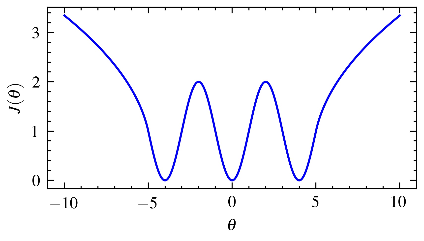
Consider the following function :
which function is depicted in Figure 1 It satisfies Assumptions (J4) and (J5), and has multiple global minima. However, if some of the local minima were to be greater than the global minimum, then (J4) and (J5) would fail to be satisfied.
Example 2.
Now suppose is is strictly convex, and suppose further that there exist constants such that
Here, for symmetric matrices , the notation means that is positive semidefinite. Since is strictly convex, is a singleton . In this case Assumptions (J4) and (J5) are satisfied trivially. Thus the theory presented here is applicable to strictly convex functions, as well as some nonconvex functions.
The algorithm for finding a stationary point of is as follows: Choose an initial guess (usually deterministic). At time , we choose a random “search direction” , which satisfies certain assumptions to be specified below. Once is chosen, is updated according to
| (3) |
Here, is a deterministic sequence of step sizes where for each . In batch updating we could, in principle, use “local clocks” to choose a different step size for each updated component, as suggested in [55]. However, in the interests of simplicity, in this paper we stick to using a global clock, so that every component that is updated uses the same step size. Batch updating means that, at any time , only some components of could be nonzero, and the rest are set to zero. Some possible options for selecting are discussed in Section 4.
Let denote the tuple , and define analogously. (Note that there is no .) Let be a filtration (that is, an increasing sequence of -algebras) such that , and the random processes up to time that are involved in selecting the nonzero components of , are all measurable with respect to . For future use, let denote the set of all functions that are measurable with respect to .
The general framework studied in [56] (which is our inspiration) is that the search direction is random, but there is a fixed constant such that
where denote the conditional expectation with respect to . Since the constant can be absorbed into the step size , we choose , and accordingly define:
| (4) |
Thus is the difference between the conditional expectation of the search direction, and the desired value . Observe that . Next, define as the “unpredictable part” of the search direction, namely
| (5) |
With this background, we make the following assumptions about the search direction :
- (D1).
There is a sequence of deterministic constants such that
(6) - (D2).
There is a sequence of deterministic constants such that
(7)
3.2 Theorem Statement
With the above assumptions, we now state the convergence theorem.
Theorem 1.
Define via (3). Then we can state the following conclusions.
- 1.
Suppose assumptions (J1) – (J3) and (D1) – (D2) are satisfied. Suppose further that
(8) Then , , and are bounded almost surely.
- 2.
Suppose that in addition to the assumptions in Item 1, we add
(9) Then
(10) - 3.
Suppose that in addition to the assumptions in Item 2, we add Assumption (J4). Then almost surely, and almost surely, as .
- 4.
Suppose that in addition to the assumptions in Item 3, we add Assumption (J5). Then almost surely as .
3.3 Proof of Main Convergence Theorem
The proof of Theorem 1 is based on the “almost supermartingale lemma” of Robbins & Siegmund Theorem [14]. That paper is rather difficult to locate. However, the same theorem is stated as Lemma 2 in [57, Section 5.2]. A recent survey of many results along similar lines is found in [58], where Lemma 1 below is stated as Lemma 4.1. The result states the following:
Lemma 1.
Suppose are stochastic processes defined on some probability space , taking values in , adapted to some filtration , satisfying
| (11) |
Define
| (12) |
Then for all , exists, and in addition,
| (13) |
In particular, if , then is bounded almost surely.
We also make use of the following result which is easy to prove, and is stated in this form in [59, Eq. (2.40)].
Lemma 2.
Suppose is and is globally Lipschtiz-continuos with constant . Then
| (14) |
We begin with a few preliminary observations. By the “tower” property of conditional expectations, it follows from (5) that
| (15) |
Therefore
| (16) | |||||
(Proof of Theorem 1:)
Item 1:
Recall the update rule (3) and apply Lemma 1.
This gives
Subtract from both sides and define . This gives
Now take conditional expectations and invoke (4), (15) and (16). This gives
Now apply Schwarz’s inquality, and assumptions (D1), (D2). This gives
Next, invoke (J3), and observe that
This leads to
After regrouping terms, the above bound is of the form (11) with
For Item 1, let us ignore because it is non-negative. Also, both and are deterministic sequences. Hence, if it can be shown that both sequences and are summable, then it would follow from Lemma 1 that converges almost surely to some random variable , and is bounded along almost all sample paths. Now (J3) implies that is also bounded almost surely, while the compactness of the level sets of implies that is bounded almost surely. Thus we focus on establishing the summability of these two sequences and .
For this purpose, we recall the hypotheses in (8). Using these, it is shown that each term in the definitions of and is summable. First, , which is the first term (modulo the constant ) in both and . Next,
which is the second term in . Next, because is bounded by one, we have
which is the second term in and the third term in .
Next, by assumption , which is the
third term in .
Last, by assumption ,
which is the fourth and final term (modulo ) in both and .
Hence both sequences are summable, which establishes Item 1.
Item 2:
Now we make use of the second part of Lemma 1, namely
Suppose there exists an such that
Choose a time such that
and observe that
Then
| (17) |
which shows that the set of such must have measure zero.
This is Item 2.
Item 3:
Now it is assumed that Assumption (J4) also holds in addition to (J3).
Define
to be the set of such that
, and observe that .
Now suppose , and define
.
Suppose by way of contradiction that , say
.
Choose sufficiently large that for all .
Then by (J4), it follows that, for all , we have
Now apply (17) with replaced by ,
which leads to a contradiction.
Hence the set of for which
has measure zero, or almost surely, and
almost surely.
Item 4:
We already know from Item 3 that almost surely.
Now apply Assumption (J5).
4 Various Batch Updating Options
In this section, we first propose some possible choices of search directions for batch updating. These include many commonly used choices. Then we analyze each of these choices, and show that they all satisfy the standard assumptions (D1) and (D2). Usually (D1) is straight-forward and the main challenge is to establish (D2). Once it is established that both (D1) and (D2) are satisfied, then one can apply Theorem 1 to conclude that the iterative algorithm (3) converges to a solution for any objective function that satisfies Assumptions (J1) through (J5), or some subset thereof, provided the step size conditions (8) and (9) are satisfied.
4.1 Various Options for Batch Updating
In this subsection we study different options that are possible to fit in our convergence theorem.
Option 1: The first of these is the standard steepest descent with possibly noise-corrupted gradient measurements. Let
| (18) |
where is a sequence of unstructured disturbances, including measurement errors. Following the usage in this area, we will refer to these as “measurement noise.” The noise is assumed to satisfy
| (19) |
| (20) |
for a known set of constants . These assumptions applies to all options studied here.
Option 2: The next option is “coordinate gradient descent” as defined in [60] and studied further in [61]. At time , choose an index at random with a uniform probability, and independently of previous choices. Let denote the elementary unit vector with a as the -th component and zeros elsewhere, and let denote the measurement noise. Then define
| (21) |
The factor of arises because the likelihood that equalling any one index is . Thus, with the introduction of the factor , it follows that if we ignore the noise term for the time being, then
Note that, though is used at time , it is chosen at time , that is, prior to the update at time . Hence .
Option 3: This is option is just coordinate gradient descent along multiple coordinates chosen at random. At time , choose different indices from with replacement, with each choice being independent of the rest, and also of past choices. Moreover, each is chosen from with uniform probability. Then define
| (22) |
where is the noise sequence. In this option, can have up to nonzero components. Because the sampling is with replacement, there might be some duplicated samples. In such a case, the corresponding component of simply gets counted multiple times in (22).
Option 4: This is a variant of coordinate gradient descent. At time , let be independent Bernoulli processes with success rate . Thus
| (23) |
It is permissible for the success probability to vary with time. However, at any one time, all components must have the same success probability. Define
| (24) |
Thus equals if , and equals otherwise. Now define
| (25) |
In this option, the search direction can have up to nonzero components. However, the expected number of nonzero components is .
Options 1A through 4A: In these options, we apply Options 1 through 4, after replacing the actual gradient , by a first-order approximation, as suggested first in [41]. Let be a predetermined sequence of “increments” (not to be confused with the step size sequence ). At each time , define the approximate gradient by
| (26) |
where are zero-mean measurement noises satisfying (34) that
| (27) |
| (28) |
for suitable constants .
4.2 Convergence Theorems
Theorem 2.
Suppose the objective function satisfies assumptions (J1)–(J5), and suppose is chosen according to any one of Options 1 through 4.
- 1.
Suppose the step size sequence satisfies
(29) Then , and are all bounded almost surely.
- 2.
If, in addition to (29), the step size sequence also satisfies
(30) then and as , almost surely as .
Note that if , a fixed constant for all , then the two conditions in (29) are equivalent. Moreover, taken together, (29) and (30) become the well-known Robbins-Monro conditions [33].
Theorem 3.
Suppose the objective function satisfies assumptions (J1)–(J5), and suppose we apply batch updating with any one of Options 1A through 4A. Under these conditions,
- 1.
Suppose that the step size sequence satisfies
(31) Then , and are all bounded almost surely.
- 2.
4.3 Analysis of Various Batch Updating Options
In this subsection, we analyze the various batch updating options in Section 4.1. To keep the notation from getting overly cumbersome, it is assumed that in Options 1 through 4, the noise satisfies
| (33) |
| (34) |
for a known set of constants . With these assumptions, each of Options 1 through 4, “on average” the search direction equals . Therefore Assumption (D1) is satisfied with for all . This is not true in Options 1A through 4A. The discussion below will reveal that more general models can be accommodated at the expense of more cumbersome notation.
In Option 2, there are two factors contributing to the error . First, even if , the search direction equals only “on average,” and there is a variance due to this. Second, the variance due to the noise also needs to be taken into account.
Let denote . Then
Therefore
Now with probability . Therefore the conditional probability
Since
if , its conditional variance simply adds to the above. Therefore (D2) is satisfied with
In Option 3, is the average of different quantities wherein the error terms are independent. Therefore their variances just add up, an again Assumption (D2) holds with .
Next we come to Option 4. For notational simplicity, we just use in the place of . In this case, each component equals with probability , and with probability . Thus equals with probability , and with probability . As can be easily verified, the variance is for each component. As the Bernoulli processes for each component are mutually independent, the variances simply add up. It follows that
Hence Assumption (D2) holds with
Finally we come to Option 1A through 4A, which is distinguished by the fact that we cannot take in general. Define by
| (35) |
Then it is clear that the search direction in (26) is given by
| (36) |
Recall from (27) and (4.1) that
| (37) |
| (38) |
for suitable constants .
Proof.
By (27), it follows that
Next, we adapt the proof of Lemma 2 taken from [59] to the problem at hand, and write
Now apply Assumption (J1) and Schwarz’s inequality. This gives
Therefore
Therefore
This proves (41). To prove (42), observe that and are independent. Therefore the conditional variance of is the sum of the conditional variances of these two terms, divided by , which is bounded by . ∎
5 Computational Results
To validate the theory, we have conducted the following numerical experiment: We set , where is a positive definite matrix with a condition number of 100, whose eigenvectors are not aligned closely with the elementary basis vectors; that is, is far from being a diagonal matrix. Four different updating options were implemented, namely: Option 1 (full gradient updating), Option 4 (batch updating with different independent Bernoulli processes with for all . The “rate” was assigned various values to measure performance.), Option 1A and Option 4A (Options 1 and 4 respectively, using an approximate gradient defined in (27) instead of the true gradient). The noise was additive white Gaussian noise with various SNRs, which determined the variance bound in (4.1). The step and increment sequences were chosen to be
where , , . With these choices, the sufficient conditions of Theorems 2 and 3 are satisfied. For comparision we set to be same in ADAM, NADAM, RMSPROP [62], and Heavy Ball (HB). For NAG, we stick to step sequences proposed in [2]. The computations were conducted in python using NumPy and PyTorch (for GPU Acceleration) libraries.
Figure 2 displays the convergence of Option 4 (batch updating of a fraction components, using noisy measurements of the true gradient), at 50dB SNR for various values of . It can be seen that, with as few as 5% of the components being updated on average (), the iterations converge.
Figure 3 shows the output of Option 1 (left side) and Option 4 with (right side). Recall that Option 1 is to update all components at each time step, while Option 4 is to update a fraction of the components, using noise-corrupted true gradients in each case. In this case, batch updating (BU) converges, albeit slowly. Five other momentum-based (or second-order) methods fail to converge, namely NAG which performs the worst, ADAM, NADAM and RMSPROP, and HB which performs least badly. Figure 4 shows the output of Option 1A (left side) and Option 4A with (right side). In this case, the noise-corrupted true gradients are replaced by approximate gradients as in (26). Here the Nesterov method actually diverges, while the others settle down at some value of the objective function, though far from the optimum. Batch updating converges to the optimum.
6 Conclusions
In this paper, we have presented a general and unified framework for establishing the convergence of batch updating algorithms. Then we have presented sufficient conditions for the convergence of these batch updating algorithms. Our method of proof is based on stochastic approximation theory, specifically [14]. The results are applicable to nonconvex as well as convex objective functions. In particular, the search direction can be a batch-updated version of any of the following:
- •
A noisy measurement of the exact gradient.
- •
A first-order approximation of the gradient based on noisy function measurements (also called zeroth-order or derivative-free methods).
Numerical experiments show that when as little as 5% of the coordinates are updated at each iteration, and approximate gradients are used, batch updating still converges, while batch momentum-based convex optimization methods either diverge or fail to converge at quite low noise levels. The existing convergence theory for momentum-based algorithms does not apply to the case of batch updating. Extending the present theory to commonly used algorithms like ADAM/NADAM is a current topic of investigation.
References
- [1] B. Polyak, “Some methods of speeding up the convergence of iteration methods,” USSR Computational Mathematics and Mathematical Physics, vol. 4, no. 5, pp. 1–17, 1964.
- [2] Y. Nesterov, “A method for unconstrained convex minimization problem with the rate of convergence (in russian),” Soviet Mathematics Doklady, vol. 269, pp. 543–547, 1983.
- [3] Y. Nesterov, Introductory Lectures on Convex Optimization: A Basic Course, vol. 87. Springer Scientific+Business Media, 2004.
- [4] I. Sutskever, J. Martens, G. Dahl, and G. Hinton, “On the importance of initialization and momentum in deep learning,” in Proceedings of the 30th International Conference on Machine Learning (S. Dasgupta and D. McAllester, eds.), vol. 28 of Proceedings of Machine Learning Research, (Atlanta, Georgia, USA), pp. 1139–1147, PMLR, 17–19 Jun 2013.
- [5] Y. Bengio, N. Boulanger-Lewandowski, and R. Pascanu, “Advances in optimizing recurrent networks,” pp. 8624–8628, 2013.
- [6] D. P. Kingma and J. Ba, “Adam: A method for stochastic optimization,” in 3rd International Conference on Learning Representations, ICLR 2015, San Diego, CA, USA, May 7-9, 2015, Conference Track Proceedings (Y. Bengio and Y. LeCun, eds.), 2015.
- [7] T. Dozat, “Incorporating nesterov momentum into adam,” 2016.
- [8] A. Barakat and P. Bianchi, “Convergence and dynamical analysis of the behavior of the ADAM algorithm for nonconvex stochastic optimization,” SIAM Journal on Optimization, vol. 31, no. 1, pp. 244–274, 2021.
- [9] K. Khamaru and M. Wainwright, “Convergence guarantees for a class of non-convex and non-smooth optimization problems,” in Proceedings of the 35th International Conference on Machine Learning (J. Dy and A. Krause, eds.), vol. 80 of Proceedings of Machine Learning Research, pp. 2601–2610, PMLR, 10–15 Jul 2018.
- [10] S. Ruder, “An overview of gradient descent optimization algorithms,” 2016.
- [11] M. Li, T. Zhang, Y. Chen, and A. J. Smola, “Efficient mini-batch training for stochastic optimization,” in Proceedings of the 20th ACM SIGKDD International Conference on Knowledge Discovery and Data Mining, KDD ’14, p. 661–670, Association for Computing Machinery, 2014.
- [12] Y. Lin, S. Han, H. Mao, Y. Wang, and B. Dally, “Deep gradient compression: Reducing the communication bandwidth for distributed training,” in International Conference on Learning Representations, 2018.
- [13] H. Noh, T. You, J. Mun, and B. Han, “Regularizing deep neural networks by noise: Its interpretation and optimization,” in Advances in Neural Information Processing Systems, vol. 30, Curran Associates, Inc., 2017.
- [14] H. Robbins and D. Siegmund, A convergence theorem for non negative almost supermartingales and some applications, pp. 233–257. Elsevier, 1971.
- [15] J. Liu and Y. Yuan, “On almost sure convergence rates of stochastic gradient methods,” in Proceedings of Thirty Fifth Conference on Learning Theory (P.-L. Loh and M. Raginsky, eds.), vol. 178 of Proceedings of Machine Learning Research, pp. 2963–2983, PMLR, 02–05 Jul 2022.
- [16] O. Sebbouh, R. M. Gower, A. Defazio, and I. Paris, “Almost sure convergence rates for stochastic gradient descent and stochastic heavy ball,” in Annual Conference Computational Learning Theory, 2021.
- [17] A. Khaled and P. Richtárik, “Better theory for sgd in the nonconvex world,” 2020.
- [18] L. Bottou, F. E. Curtis, and J. Nocedal, “Optimization methods for large-scale machine learning,” SIAM Review, vol. 60, no. 2, pp. 223–311, 2018.
- [19] P. Mertikopoulos, N. Hallak, A. Kavis, and V. Cevher, “On the almost sure convergence of stochastic gradient descent in non-convex problems,” in Advances in Neural Information Processing Systems (H. Larochelle, M. Ranzato, R. Hadsell, M. Balcan, and H. Lin, eds.), vol. 33, pp. 1117–1128, Curran Associates, Inc., 2020.
- [20] H. Wang, M. Gurbuzbalaban, L. Zhu, U. Simsekli, and M. A. Erdogdu, “Convergence rates of stochastic gradient descent under infinite noise variance,” in Advances in Neural Information Processing Systems (A. Beygelzimer, Y. Dauphin, P. Liang, and J. W. Vaughan, eds.), 2021.
- [21] M. Crawshaw, M. Liu, F. Orabona, W. Zhang, and Z. Zhuang, “Robustness to unbounded smoothness of generalized signSGD,” in Advances in Neural Information Processing Systems (A. H. Oh, A. Agarwal, D. Belgrave, and K. Cho, eds.), 2022.
- [22] B. Fehrman, B. Gess, and A. Jentzen, “Convergence rates for the stochastic gradient descent method for non-convex objective functions,” Journal of Machine Learning Research, vol. 21, no. 136, pp. 1–48, 2020.
- [23] X. Li and F. Orabona, “On the convergence of stochastic gradient descent with adaptive stepsizes,” in Proceedings of the Twenty-Second International Conference on Artificial Intelligence and Statistics, vol. 89 of Proceedings of Machine Learning Research, pp. 983–992, PMLR, 16–18 Apr 2019.
- [24] P. Tseng, “Convergence of a block coordinate descent method for nondifferentiable minimization,” Journal of optimization theory and applications, vol. 109, no. 3, pp. 475–494, 2001.
- [25] Y. Nesterov, “Efficiency of coordinate descent methods on huge-scale optimization problems,” SIAM Journal on Optimization, vol. 22, no. 2, pp. 341–362, 2012.
- [26] P. Richtárik and M. Takávc, “Iteration complexity of randomized block-coordinate descent methods for minimizing a composite function,” Mathematical Programming, vol. 144, pp. 1–38, Dec. 2012.
- [27] P. Richtárik and M. Takávc, “Parallel coordinate descent methods for big data optimization,” Mathematical Programming, vol. 156, pp. 433–484, Apr. 2015.
- [28] Z. Lu and L. Xiao, “On the complexity analysis of randomized block-coordinate descent methods,” Mathematical Programming, vol. 152, pp. 615–642, Aug. 2014.
- [29] J. C. Spall, “Cyclic Seesaw Process for Optimization and Identification,” Journal of Optimization Theory and Applications, vol. 154, no. 1, pp. 187–208, 2012.
- [30] K. Hernandez and J. C. Spall, “Cyclic stochastic optimization with noisy function measurements,” 2014 American Control Conference, pp. 5204–5209, 2014.
- [31] K. Hernandez and J. C. Spall, “Asymptotic Normality and Efficiency Analysis of the Cyclic Seesaw Stochastic Optimization Algorithm,” 2016 American Control Conference (ACC), pp. 7255–7260, 2016.
- [32] K. Hernandez, “Cyclic Stochastic Optimization via Arbitrary Selection Procedures for Updating Parameters,” 2016 Annual Conference on Information Science and Systems (CISS), pp. 349–354, 2016.
- [33] H. Robbins and S. Monro, “A stochastic approximation method,” Annals of Mathematical Statistics, vol. 22, no. 3, pp. 400–407, 1951.
- [34] J. Wolfowitz, “On the stochastic approximation method of Robbins and Monro,” Annals of Mathematical Statistics, vol. 23, no. 3, pp. 457–461, 1952.
- [35] V. Borkar, Stochastic Approximation: A Dynamical Systems Viewpoint. Texts and Readings in Mathematics, Hindustan Book Agency, 2009.
- [36] Y. Xu and W. Yin, “Block stochastic gradient iteration for convex and nonconvex optimization,” SIAM Journal on Optimization, vol. 25, no. 3, pp. 1686–1716, 2015.
- [37] B. Recht, C. Re, S. Wright, and F. Niu, “Hogwild!: A lock-free approach to parallelizing stochastic gradient descent,” in Advances in Neural Information Processing Systems (J. Shawe-Taylor, R. Zemel, P. Bartlett, F. Pereira, and K. Weinberger, eds.), vol. 24, Curran Associates, Inc., 2011.
- [38] J. Chen, R. Monga, S. Bengio, and R. Jozefowicz, “Revisiting distributed synchronous sgd,” in International Conference on Learning Representations Workshop Track, 2016.
- [39] C. Xie, S. Koyejo, and I. Gupta, “Zeno++: Robust fully asynchronous SGD,” in Proceedings of the 37th International Conference on Machine Learning (H. D. III and A. Singh, eds.), vol. 119 of Proceedings of Machine Learning Research, pp. 10495–10503, PMLR, 13–18 Jul 2020.
- [40] L. Nguyen, P. H. NGUYEN, M. van Dijk, P. Richtarik, K. Scheinberg, and M. Takac, “SGD and hogwild! Convergence without the bounded gradients assumption,” in Proceedings of the 35th International Conference on Machine Learning (J. Dy and A. Krause, eds.), vol. 80 of Proceedings of Machine Learning Research, pp. 3750–3758, PMLR, 10–15 Jul 2018.
- [41] J. Kiefer and J. Wolfowitz, “Stochastic estimation of the maximum of a regression function,” Annals of Mathematical Statistics, vol. 23, no. 3, pp. 462–466, 1952.
- [42] J. R. Blum, “Multivariable stochastic approximation methods,” Annals of Mathematical Statistics, vol. 25, no. 4, pp. 737–744, 1954.
- [43] J. C. Spall, “An overview of the simultaneous perturbation method for efficient optimization,” Johns Hopkins apl technical digest, vol. 19, no. 4, pp. 482–492, 1998.
- [44] A. T. Vakhitov, O. N. Granichin, and L. S. Gurevich, “Algorithm for stochastic approximation with trial input perturbation in the nonstationary problem of optimization,” Automation and Remote Control, vol. 70, pp. 1827–1835, Nov. 2009.
- [45] J. C. Spall, “A one-measurement form of simultaneous perturbation stochastic approximation,” Automatica, vol. 33, no. 1, pp. 109–112, 1997.
- [46] Y. Nesterov and V. Spokoiny, “Random gradient-free minimization of convex functions,” Foundations of Computational Mathematics, vol. 17, pp. 527–566, Nov. 2015.
- [47] Y. Wang, S. Du, S. Balakrishnan, and A. Singh, “Stochastic zeroth-order optimization in high dimensions,” in Proceedings of the Twenty-First International Conference on Artificial Intelligence and Statistics (A. Storkey and F. Perez-Cruz, eds.), vol. 84 of Proceedings of Machine Learning Research, pp. 1356–1365, PMLR, 09–11 Apr 2018.
- [48] H. Cai, D. McKenzie, W. Yin, and Z. Zhang, “Zeroth-order regularized optimization (zoro): Approximately sparse gradients and adaptive sampling,” SIAM Journal on Optimization, vol. 32, no. 2, pp. 687–714, 2022.
- [49] H. Cai, D. McKenzie, W. Yin, and Z. Zhang, “A one-bit, comparison-based gradient estimator,” Applied and Computational Harmonic Analysis, vol. 60, pp. 242–266, sep 2022.
- [50] H. Cai, Y. Lou, D. Mckenzie, and W. Yin, “A zeroth-order block coordinate descent algorithm for huge-scale black-box optimization,” in Proceedings of the 38th International Conference on Machine Learning (M. Meila and T. Zhang, eds.), vol. 139 of Proceedings of Machine Learning Research, pp. 1193–1203, PMLR, 18–24 Jul 2021.
- [51] H. Mohammadi, M. Razaviyayn, and M. R. Jovanović, “Performance of noisy nesterov’s accelerated method for strongly convex optimization problems,” in 2019 American Control Conference (ACC), pp. 3426–3431, 2019.
- [52] A. Barakat and P. Bianchi, “Convergence and dynamical behavior of the adam algorithm for nonconvex stochastic optimization,” SIAM Journal on Optimization, vol. 31, no. 1, pp. 244–274, 2021.
- [53] M. Assran and M. Rabbat, “On the convergence of nesterov’s accelerated gradient method in stochastic settings,” in Proceedings of the 37th International Conference on Machine Learning, ICML’20, JMLR.org, 2020.
- [54] M. Vidyasagar, “Convergence of Stochastic Approximation via Martingale and Converse Lyapunov Methods.” arxiv:2205.01303v3, January 2023.
- [55] V. S. Borkar, “Asynchronous stochastic approximations,” SIAM Journal on Control and Optimization, vol. 36, no. 3, pp. 840–851, 1998.
- [56] B. T. Polyak and Y. Z. Tsypkin, “Pseudogradient adaptation and training algorithms,” Automation and Remote Control, vol. 34, no. 3, pp. 377–397, 1973.
- [57] A. Benveniste, M. Metivier, and P. Priouret, Adaptive Algorithms and Stochastic Approximation. Springer-Verlag, 1990.
- [58] B. Franci and S. Grammatico, “Convergence of sequences: A survey,” Annual Reviews in Control, vol. 53, pp. 1–26, 2022.
- [59] D. P. Bertsekas and J. N. Tsitsiklis, “Global convergence in gradient methods with errors,” SIAM Journal on Optimization, vol. 10, no. 3, pp. 627–642, 2000.
- [60] S. J. Wright, “Coordinate descent algorithms,” Mathematical Programming, vol. 151, no. 1, pp. 3–34, 2015.
- [61] S. Vaswani, F. Bach, and M. Schmidt, “Fast and Faster Convergence of SGD for Over-Parameterized Models (and an Accelerated Perceptron),” in Proceedings of the 22nd International Conference on Artificial Intelligence and Statistics (AISTATS), pp. 1–10, 2019.
- [62] T. Tieleman, G. Hinton, et al., “Lecture 6.5-rmsprop: Divide the gradient by a running average of its recent magnitude,” COURSERA: Neural networks for machine learning, vol. 4, no. 2, pp. 26–31, 2012.