The E-Bayesian Estimation and its E-MSE of Lomax distribution under different loss functions

Lomax distribution is a widely used life distribution in reliability and life test research, especially in the analysis of life test data processing in medicine, biological sciences, and engineering sciences. This distribution has monotonically increasing and decreasing failure rates.

The probability density function (PDF) of Lomax distribution is as follows:

Hence, the cumulative distribution function (CDF) is given by

where $\alpha$ is the shape parameter and $\lambda$ is the scale parameter. The reliability function $R(t)$ and the hazard rate function $h(t)$ for Lomax distribution are, respectively, given by

and

When $X\sim Lomax(\alpha,\lambda)$, the expection of $X$ is

and the variance of $X$ is

The line charts of the probability density function of Lomax distribution are shown in Figure 1 and Figure 2.

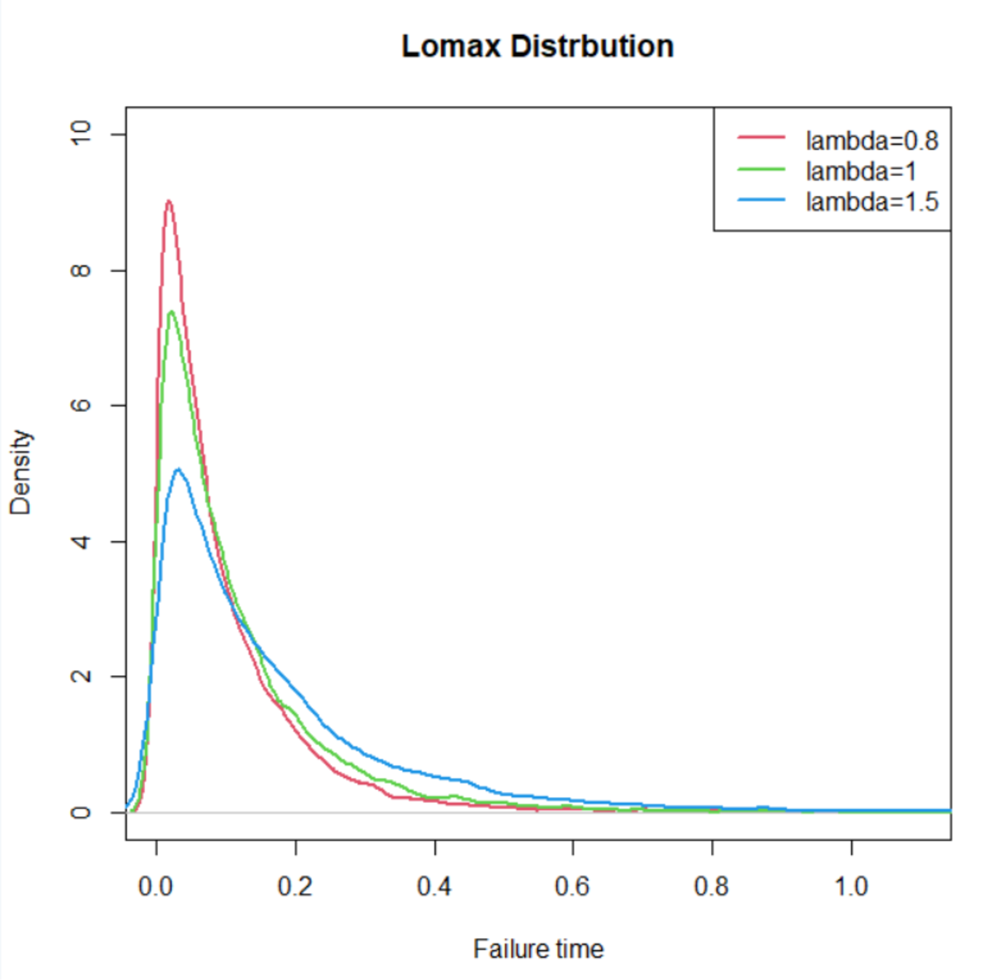
When it comes to Figure 1 and Figure 2, the plots of the probability density functions, we can observe the characteristics of the line charts under the different values of $\alpha$ and $\lambda$. We get the charts when $\alpha=8,10,12$ as $\lambda=1$ and when $\lambda=0.8,1,1.5$ as $\alpha=10$. The probability density is concentrated in places where the value of time is smaller as the parameter $\alpha$ increases. And as the parameter $\lambda$ increases, probability density decreases in places where the value of time is smaller.

If $x=(x_{1},x_{2},\cdots,x_{n})$ is a set of samples obeying the Lomax distribution, when the shape parameter is unknown and the scale parameter is known, the likelihood function is as follows:

where $T=\displaystyle\sum_{i=1}^{n}\ln(1+\frac{x_{i}}{\lambda})$.

The parameters of the Lomax distribution can be estimated in different ways under different conditions. Labban 2019 discussed the two-parameter estimation of Lomax distribution. Al-Sobhi & Al-Zahrani 2013 gave the estimation of the parameters of Lomax distribution under general progressive censoring.

At the same time, composite distribution functions of Lomax distribution have been studied too. Cordeiro et al. 2015 and Alzahrani & Sagor 2014 gave the research of the Gamma-Lomax distribution and the Poisson-Lomax distribution. Almetwally & Almongy 2020 gave the parameter estimation and stress-strength model of power Lomax distribution.

Different estimation methods are used in this paper. Each method has its own disadvantages, such as computational complexity, estimation error and so on. Therefore, a new method, E-Bayesian method, is used in this study.

Bayesian statistical inference method depends on the choice of prior distribution and loss function. But the prior distribution parameter may depend on the hyperparameters. In this case, we usually use the hierarchical Bayesian method. Smith & Lindleya. 1972 first proposed the idea of the hierarchical prior distribution. The hierarchical Bayesian method needs two stages to complete the setting of the prior distribution, so it is more robust than the Bayesian method. Han 1997 proposed a method to construct hierarchical prior distribution. Recently, the hierarchical Bayesian method has been applied to data analysis. For more details, refer to Arnold & Tomohiro 2010. However, hierarchical Bayesian estimation often involves the calculation of complex integrals. In practical application, it is difficult to use the hierarchical Bayesian method to calculate integrals. Some calculation methods such as the Markov chain Monte Carlo (MCMC) method are available especially the Metropolis-Hastings (MH) algorithm. For more details we can refer to Hastings 1970 and Cowles & Carlin. 1995.

On the other hand, loss function plays an important role in Bayesian methods. In Bayesian reasoning, square error loss is most commonly used. This kind of loss function is symmetrical and gives equal weight to both overestimation and underestimation. It is well known that in many cases, it may not be appropriate to use symmetric loss function, especially when positive error and negative error have different consequences. One of the most commonly used asymmetric loss functions is the LINEX (linear exponential) loss function. Varian 1975 introduced this point, and Zellner 1986 studied the further properties of this loss function. In many practical cases, it seems more realistic to express loss by ratio. In this case, Parsian & Nematollahi 1996 pointed out that another useful asymmetric loss function is the entropy loss function. For parameter estimation under entropy loss function, see Parsian & Nematollahi 1996. Research on Bayesian estimation under different loss functions is given in Han 2018.

The E-Bayesian estimation of parameters of Lomax distribution based on different loss functions is studied in this article.

In this section, we will calculate the Bayesian estimation of alpha under three loss functions. According to Ali et al. 2013, let $x=(x_{1},x_{2},\cdots,x_{n})$ be a set of samples obeying the Lomax distribution, for any prior distribution of parameter $\alpha$, have the following conclusions:

1. 1)

   Under the square error loss (SEL) function, $L_{1}(\alpha,\delta)=(\alpha-\delta)^{2}$, the Bayesian estimation of $\alpha$ is $\hat{\alpha}_{B1}(x)=E(\alpha|x)$.

2. 2)

   Under the K-loss (KL) function, $L_{2}(\alpha,\delta)=(\sqrt{\alpha/\delta}-\sqrt{\delta/\alpha})^{2}$, the Bayesian estimation of $\alpha$ is $\hat{\alpha}_{B2}(x)=\sqrt{{E(\alpha|x)}/{E(\alpha^{-1}|x)}}$.

3. 3)

   Under the entropy loss (EL) function, $L_{3}(\alpha,\delta)=\delta/\alpha-\ln(\delta/\alpha)-1$, the Bayesian estimation of $\alpha$ is $\hat{\alpha}_{B3}(x)=[E(\alpha^{-1}|x)]^{-1}$.

In this section, we consider that the Bayesian estimation of the unknown parameter $\alpha$ is based on the above loss functions. The Bayesian approach requires the specification of the prior PDF of the parameter $\alpha$. Because $\alpha>0,\lambda>0$, it is assumed that the PDF of Gamma distribution is the prior PDF as follows:

When $\lambda$ is fixed, and $X=(X_{1:n},X_{2:n},\cdots,X_{n:n})$, $x=(x_{1:n},x_{2:n},\cdots,x_{n:n})$, from (2.2) and (2.3), the posterior PDF of $\alpha$ is given as follows:

So we can get the Bayesian estimation of $\alpha$ under three loss functions.

According to Han 1997, the prior parameters $a$ and $b$ should be selected to guarantee that $\pi(\alpha)$ is a decreasing function of $\alpha$. The derivative of $\pi(\alpha)$ with respect to $\alpha$ is given by

where $\Gamma(a)=\int_{0}^{+\infty}x^{a-1}e^{-x}dx$ is the gamma function, and hyper parameters $a>0$ and $b>0$.

The prior PDF $\pi(\alpha)$ is a decreasing function of $\alpha$. We can assume that the hyperparameters called $a$ and $b$ are independent with bi-variate PDF given by

We define that $a>0,b>0$, and $\alpha>0$, it follows $0<a<1,b>0$ due to $\frac{d\pi(\alpha)}{d\alpha}<0$, and therefore $\pi(\alpha|a,b)$ is a decreasing function of $\lambda$. Given $0<a<1$, the larger $b$ is, the thinner the tail of the Gamma density function will be. Considering the robustness of Bayesian estimate in Berger & James 1985, the thinner tailed prior distribution often reduces the robustness of Bayesian estimate. Accordingly, $b$ should not be larger then a given upper bound $c$, where $c>0$ is a constant to be determined. Thereby, the hyper parameters $a$ and $b$ should be selected with the restriction of $0<a<1$ and $0<b<c$. How to determine the constant $c$ would be described later in application example.

The E-Bayesian estimation of the parameter $\alpha$ is given by

in which $Q$ is the set of all possible values of the parameters $a$ and $b$. $\hat{\alpha}_{B}(a,b)$ is the Bayesian estimations of the parameter $\alpha$. We indicates that $\hat{\alpha}_{EB}=E[\hat{\alpha}_{B}(a,b)]$.

If $X_{1},X_{2},\cdots,X_{n}$ are the failure sample observations from the Lomax distribution (1.1), the likelihood function is given by (1.7), the prior density function $\pi(\alpha|a,b)$ of $\alpha$ is given by (2.2). Refer to Han 2020, the prior density function $\pi(a,b)$ of $a$ and $b$ is given by

The definition of E-Bayesian estimation was originally addressed by Han 2007.

We usually use MSE (mean square error) to measure the estimated error. The E-Bayesian estimation method proposed time is short, the research results obtained are also less, especially the analytical expression of its estimated error has not been studied. Han 2019a in the case of the two hyperparameters, proposed the definition of E-MSE. Han 2019b in the case of the one hyperparameter, proposed the definition of E-MSE (expected mean square error), too. From which we get the MSE of Bayesian estimation of $\hat{\alpha}_{BS}(a,b)$ as

So we can fix the E-Bayesian estimation of MSE called E-MSE as follows:

which is the E-MSE (expected mean square error)) of E-Bayesian estimation $\hat{\alpha}_{EB}(a,b)$ where $Q$ is the domain of a and b, $MSE[\hat{\alpha}_{B}(a,b)]$ is the MSE of Bayesian estimation of $\alpha$ with hyper parameters $a$ and $b$, and $\pi(a,b)$ is the density function of $a$ and $b$ over $Q$. We indicates that $E-MSE[\hat{\alpha}_{EB}(a,b)]=E\{MES[\hat{\alpha}_{B}(a,b)]\}$.

In this section, we will introduce the E-Bayesian estimation of $\alpha$ under different loss functions according to Han 2020.

In this section, the Monte Carlo simulation is used to compare the E-Bayesian estimation and its E-MSE under different loss functions. For known values of $\lambda=1,2,3$ and $\alpha=2.5$, a sample of size $n$ is then generated from the Lomax distribution by using the inverse function method as follows:

in which $U$ is generated from U(0,1). The codes of R are used to generate datasets from the uniform and Lomax distributions.

The performance of all estimations are compared numerically by their $\hat{\alpha}_{EBi}$ and $E-MSE(\hat{\alpha}_{EBi})$ $(i=1,2,3)$ values. The simulation results with 10000 repetitions are given in table 1-3 $(c=0.5,1,1.5)$.

Similarly, for known values of $\lambda=1,2,3$ and $\alpha=5.0$, a sample of size $n$ is then generated from the Lomax distribution by using the inverse function method too. The performance of all estimates are compared numerically by their $\hat{\alpha}_{EBi}$ and $E-MSE(\hat{\alpha}_{EBi})$ $(i=1,2,3)$ values. The simulation results with 10000 repetitions are given in table 4-6 $(c=0.5,1,1.5)$. Based on tabulated the values of $E-MSE(\hat{\alpha}_{EBi})$ $(i=1,2,3)$ $(i=1,2,3)$, the following conclusions can be drawn from Tables 1–3 or Tables 4–6 (c = 0.5, 1, 1.5).

1. (1)

   Based on different loss functions, for the fixed $c(c=0.5,1,1.5)$, it is observed that by the increasing of $n$, the performances of all estimations improve in terms of $\hat{\alpha}_{EBi}$ and $E-MSE(\hat{\alpha}_{EBi})$ $(i=1,2,3)$.

2. (2)

   For the same values of $n(n=20,40,60,80,100)$ and the different values of $c(c=0.5,1,1.5)$, the values of $\hat{\alpha}_{EBi}$ and $E-MSE(\hat{\alpha}_{EBi})$ $(i=1,2,3)$ are all robust.

3. (3)

   For the same $n(n=20,40,60,80,100)$ and $c(c=0.5,1,1.5)$, the values of $\hat{\alpha}_{EBi}$ are close to each other, the values of $E-MSE(\hat{\alpha}_{EBi})$ $(i=1,2,3)$ are close to

It also suggests that, if E-MSE as the evaluation standard, then have conclusions as follows: $\hat{\alpha}_{EB1}$ is more accurate than $\hat{\alpha}_{EB2}$, and $\hat{\alpha}_{EB2}$ is more accurate than $\hat{\alpha}_{EB3}$.

References

- (1)
- Al-Sobhi & Al-Zahrani (2013) Al-Sobhi, M. & Al-Zahrani, B. (2013), ‘On parameters estimation of Lomax distribution under general progressive censoring’, Journal of Quality and Reliability Engineering 2013(5), 7.
- Ali et al. (2013) Ali, S., Aslam, M. & Kazmi, S. M. A. (2013), ‘A study of the effect of the loss function on bayes estimate, posterior risk and hazard function for lindley distribution - sciencedirect’, Applied Mathematical Modelling 37(8), 6068–6078.
- Almetwally & Almongy (2020) Almetwally, E. M. & Almongy, H. M. (2020), ‘Parameter estimation and stress-strength model of Power Lomax distribution: Classical methods and Bayesian estimation’, Journal of Data Science 18(4), 718–738.
- Alzahrani & Sagor (2014) Alzahrani, B. & Sagor, H. (2014), ‘The Poisson-Lomax distribution’, Revista Colombiana De Estadistica 37(1), 223–243.
- Arnold & Tomohiro (2010) Arnold, Z. & Tomohiro, A. (2010), ‘A direct monte carlo approach for bayesian analysis of the seemingly unrelated regression model’, Journal of Econometrics 159(1), 33–45.
- Bennett & Filliben (2000) Bennett, H. S. & Filliben, J. J. (2000), ‘A systematic approach for multidimensional, closed-form analytic modeling: Minority electron mobilities in heterostructures’, Journal of Research of the National Institute of Standards and Technology 105(3), 441–452.
- Berger & James (1985) Berger & James, O. (1985), Statistical decision theory and Bayesian analysis, New York (NY): Springer-Verlag.
- Cordeiro et al. (2015) Cordeiro, G. M., Ortega, E. M. M. & Popovic, B. V. (2015), ‘The Gamma-Lomax distribution’, Journal of Statistical Computation and Simulation 85(1-3), 305–319.
- Cowles & Carlin. (1995) Cowles, M. K. & Carlin., B. P. (1995), ‘Markov chain Monte Carlo diagnostics: A comparative review’, Journal of American Statistical Association 91(434), 883–904.
- Han (1997) Han, M. (1997), ‘The structure of hierarchical prior distribution and its applications’, Chinese Operation Research and Management Science 6, 31–40.
- Han (2007) Han, M. (2007), ‘E-bayesian estimation of failure probability and its application’, Math Comput Model 45(9-10), 1272–1279.
- Han (2018) Han, M. (2018), ‘E-bayesian estimations of the reliability and its e-posterior risk under different loss functions’, Communication in Statistics- Simulation and Computation pp. 1–19.
- Han (2019a) Han, M. (2019a), ‘E-bayesian estimation and its E-MSE under the scaled squared error loss function, forexponential distribution as example’, Communication in Statistics- Simulation and Computation 48(6), 1880–1890.
- Han (2019b) Han, M. (2019b), ‘E-bayesian estimation of parameter and its evaluation standard: E-MSE (expectedmean square error) under different loss functions’, Communication in Statistics- Simulation and Computation pp. 1–18.
- Han (2020) Han, M. (2020), ‘The E-Bayesian estimation and its E-MSE of Pareto distribution parameter under different loss functions’, Journal of Statistical Computation and Simulation 90(10), 1834–1848.
- Hastings (1970) Hastings, W. K. (1970), ‘Monte Carlo sampling methods using Markov Chains and their application’, Biometrika 57(1), 97–109.
- Labban (2019) Labban, J. A. (2019), ‘On 2-parameter estimation of Lomax distribution’, Journal of Physics Conference Series 1294, 032018.
- Lopes (2014) Lopes, R. H. C. (2014), ‘Kolmogorov–smirnov test’, International Encyclopedia of Statistical Science 10(1), 718–720.
- Parsian & Nematollahi (1996) Parsian, A. & Nematollahi, N. (1996), ‘Estimation of scale parameter under entropy loss function’, Journal of Statistical Planning and Inference 52(1), 77–91.
- Smith & Lindleya. (1972) Smith, D. V. & Lindleya., F. M. (1972), ‘Bayes estimates for the linear model’, Journal of the Royal Statistical Society 34(1), 1–41.
- Varian (1975) Varian, H. R. (1975), A bayesian approach to real estate assessment, in S. E. Feinberge & A. Zellner, eds, ‘Studies in Bayesian econometrics and statistics in Honor of Leonard’, Amsterdam:North Holland, p. 195–208.
- Zellner (1986) Zellner, A. (1986), ‘Bayesian estimation and prediction using asymmetric loss functions’, Journal of the American Statistical Association 81(394), 446–451.