Non-iterative generation of an optimal mesh for a blade passage using deep reinforcement learningJournal: arXiv

The conventional single-condition (SC) optimization problem is defined as follows:

where $\boldsymbol{x}$ is a decision vector and $f$ is a real-valued objective function. $\boldsymbol{\Omega}$ is the decision space which is defined as the set $\{\boldsymbol{x}|~g_{l}(\boldsymbol{x})\leq 0,l=1,2,\ldots,m\}$. $g_{l}(\boldsymbol{x})$ is a constraint function that determines the feasible region of $\boldsymbol{x}$, and $m$ is the number of the constraints of $\boldsymbol{x}$. The goal of SC optimization is to find an optimal solution $\boldsymbol{x}^{*}$ that maximizes $f$.

In contrast to SC optimization, a condition vector $\boldsymbol{c}$ and a condition space $\boldsymbol{\Phi}$ are introduced in MC optimization. An MC optimization problem is defined as follows:

where $\boldsymbol{\Phi}$ is defined as the set $\{\boldsymbol{c}|~h_{p}(\boldsymbol{c})\leq 0,~p=1,2,\ldots,q\}$. $h_{p}(\boldsymbol{c})$ is a constraint function that determines the feasible region of $\boldsymbol{c}$, and $q$ is the number of the constraints of $\boldsymbol{c}$. The goal of an MC optimization is to find optimal solutions $\boldsymbol{x}^{*}(\boldsymbol{c})$ that maximize $f$ as a function of $\boldsymbol{c}$.

DRL is a process of learning an optimal behavior for a complex decision-making process [18]. In the context of the present study, DRL refers to a process of learning an optimal behavior for determining the meshing parameters as a function of the blade geometry. At each discrete step $t$, an action $\boldsymbol{a}_{t}\in\mathcal{A}$ is determined based on a deterministic policy $\boldsymbol{\pi}:\mathcal{S}\rightarrow\mathcal{A}$ for a given state $\boldsymbol{s}_{t}\in\mathcal{S}$, where $\mathcal{S}$ and $\mathcal{A}$ denote state and action spaces, respectively. After taking the action $\boldsymbol{a}_{t}$, a reward $r_{t}(\boldsymbol{s}_{t},\boldsymbol{a}_{t})\in\mathbb{R}$ is obtained, and the next state $\boldsymbol{s}_{t+1}$ is determined based on a probability distribution $p(\boldsymbol{s}_{t+1}|\boldsymbol{s}_{t},\boldsymbol{a}_{t}):\mathcal{S}\times\mathcal{A}\rightarrow\mathcal{P(\mathcal{S})}$, where $\mathcal{P}(\mathcal{S})$ denotes the set of probability distributions over the state space $\mathcal{S}$. The process is repeated until the terminal step $T$, at which point one episode ends. The return $R_{t}$ is defined as the sum of an immediate reward $r_{t}$ and discounted future rewards as follows:

where $\gamma\in[0,1]$ is a discount factor that determines the weight between short-term and long-term rewards.

In DRL, the policy $\boldsymbol{\pi}_{\boldsymbol{\phi}}$ is represented by a nonlinear neural network with network parameters $\boldsymbol{\phi}$, i.e. weights and biases, that are adjusted during the training process. The goal of DRL is to find an optimal policy $\boldsymbol{\pi}_{\boldsymbol{\phi}^{*}}$ that maximizes an objective function $J$ defined as the expectation of the return. Thus, $\boldsymbol{\pi}_{\boldsymbol{\phi}}$ is updated by $\nabla_{\boldsymbol{\phi}}J$ which is calculated using the deterministic policy gradient algorithm [19] by applying the chain rule to $J$ as follows:

where $Q(\boldsymbol{s}_{t},\boldsymbol{a}_{t})$ is an action value function defined as follows:

A DRL-based MC optimization method was proposed by Kim et al. [17]. The method employs a single-step DRL [20] to address the MC optimization problem. In the single-step DRL, each learning episode consists of a single step. Given a state $\boldsymbol{s}_{t}$ at step $t$, an action $\boldsymbol{a}_{t}$ is determined, and a reward $r_{t}(\boldsymbol{s}_{t},\boldsymbol{a}_{t})$ is obtained. The episode is then terminated without being transitioned to a subsequent state. Since there are no subsequent steps, the return $R_{t}$ and the action value function $Q(\boldsymbol{s}_{t},\boldsymbol{a}_{t})$ are defined solely by the immediate reward $r_{t}$ as follows:

where the subscript $t$ is omitted as there is only one step. Using the deterministic policy gradient algorithm in Eq. (4), learning proceeds to find the optimal policy $\boldsymbol{\pi}_{\boldsymbol{\phi}^{*}}(\boldsymbol{s})$ that maximizes the immediate reward $r$. Thus, by setting the state, action, and reward of the single-step DRL as $\boldsymbol{c}$, $\boldsymbol{x}$, and $f$, respectively, learning $\boldsymbol{x}^{*}$ that maximizes $f$ as a function of $\boldsymbol{c}$ becomes possible. Consequently, $\boldsymbol{x}^{*}(\boldsymbol{c})$, the solution to the MC optimization problem, is obtained.

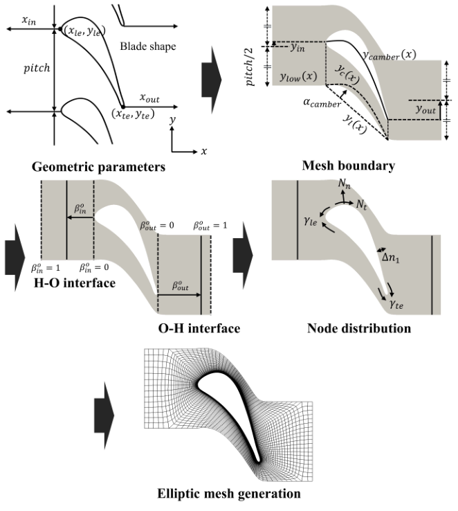
In this section, an elliptic mesh generator to generate a structured mesh for a two-dimensional blade passage is developed. The mesh generator employs an elliptic mesh generation method [21, 22] to produce an HOH-type mesh that adopts H-type meshes for the inlet and outlet sides and an O-type mesh near the blade based on the geometric parameters of the blade passage and the meshing parameters. The parameters and descriptions are listed in Table 1.

The schematic of the mesh generator is shown in Fig. 1. Firstly, the geometric parameters of the blade passage, including the blade shape, the blade $pitch$, the inlet position $x_{in}$, and the outlet position $x_{out}$, are given to the mesh generator. Subsequently, the mesh boundary is determined based on three meshing parameters $y_{in}$, $y_{out}$, and $\alpha_{camber}$. $y_{in}$ and $y_{out}$ are positions of the inlet and the outlet in the vertical direction, respectively. $\alpha_{camber}$ determines the degree to which the curvature of the lower boundary follows the camber line. The lower boundary $y_{low}(x)$ is defined as follows:

Here, $(x_{le},y_{le})$ and $(x_{te},y_{te})$ are the coordinates of the leading and trailing edges, respectively. $y_{c}(x)$ is a scaled camber line in the vertical direction defined as follows:

where $y_{camber}(x)$ is the camber line of the blade. $y_{l}(x)$ is a straight line linearly connecting two points, $(x_{le},y_{le}+y_{in}-pitch/2)$ and $(x_{te},y_{te}+y_{out}-pitch/2)$. The upper boundary is determined by shifting the lower boundary vertically by $pitch$ to ensure periodicity. Then, locations of the interface between the O-type mesh and the H-type mesh at the inlet and outlet sides are determined as $x=x_{le}-\beta^{o}_{in}~x_{in}$ and $x=x_{te}+\beta^{o}_{out}~x_{out}$, respectively.

Nodes of the O-type mesh are distributed according to $N_{t}$, $N_{n}$, $\gamma_{le}$, $\gamma_{te}$, and $\Delta n_{1}$. $N_{t}$ and $N_{n}$ are the numbers of nodes of the O-type mesh in tangential and normal directions to the blade surface, respectively. Along the blade surface, $N_{t}$ is divided so that the numbers of nodes on the pressure and suction sides are proportional to their lengths. On each side, the nodes are clustered at the leading and trailing edges for higher resolution, as shown in Fig. 2(a). Equally distributed nodes are transformed using a hyperbolic tangent function, where $\gamma_{le}$ and $\gamma_{te}$ determine the degrees of clustering at the leading and trailing edges, respectively. The transformed nodes are linearly scaled and distributed along the pressure and suction sides of a blade.

Then, edges are generated by extending the nodes on the blade surface to the outer boundary of the O-type mesh in an outward normal direction. Thereafter, the nodes at the outer boundary are adjusted such that the nodes at the upper and lower boundaries are periodically matched. Along the edge connecting the blade surface to the outer boundary of the O-type mesh, $N_{n}$ nodes are distributed. The nodes are clustered at the blade surface following a hyperbolic tangent function, as shown in Fig. 2(b). The degree of clustering is determined such that the height of the first cell at the blade surface is equal to the specified height of the first cell $\Delta n_{1}$.

After distributing the nodes of the O-type mesh, an elliptic mesh generation method [21, 22] is applied to adjust the node distribution. The elliptic mesh generation method used in the present study is proposed by Hsu and Lee [23]. It generates a mesh with high orthogonality near the blade surface without slope discontinuity inside the mesh domain. The method employs Poisson equations defined as follows:

where $(\xi,\eta)$ is the curvilinear coordinate such that the domain of $(x,y)$ is transformed into a rectangular domain. The boundaries of the rectangular domain are denoted by $\xi=0$, $\xi=\xi_{max}$, $\eta=0$, and $\eta=\eta_{max}$. The terms $P_{1}$ and $P_{2}$ are control functions that control the node distribution. By interchanging the dependent and independent variables, Eqs. (9) and (10) are transformed as follows:

where,

The values of the control functions at the boundaries $P_{1}(\xi,0)$, $P_{2}(\xi,0)$, $P_{1}(\xi,\eta_{max})$, and $P_{2}(\xi,\eta_{max})$ are determined by applying orthogonality conditions to Eqs. (11) and (12). Then, control functions inside the domain are interpolated based on power-law functions as follows:

After generating the O-type mesh using the elliptic generation method, an HOH-type mesh is eventually generated by adding H-type meshes at the inlet and outlet sides. The H-type meshes consist of cells with zero expansion ratio along both horizontal and vertical directions to ensure consistent resolution and minimize the numerical dissipation.

The MC optimization problem is solved using DRL to train the mesh generator such that it can generate an optimal mesh for various blade passages without iteration. For DRL, the actor-critic method [45] is employed. An actor $\boldsymbol{\pi}_{\boldsymbol{\phi}}$ and a critic $Q_{\boldsymbol{\zeta}}$ are functions parameterized using nonlinear neural networks. The network parameters $\boldsymbol{\phi}$ and $\boldsymbol{\zeta}$ correspond to the weights and the biases of the actor and critic networks, respectively. The actor network $\boldsymbol{\pi}_{\boldsymbol{\phi}}(\boldsymbol{s})$ determines an optimal action that maximizes the expectation of the return in Eq. (3) according to the given state. The critic network $Q_{\boldsymbol{\zeta}}(\boldsymbol{s},\boldsymbol{a})$ predicts the action value function in Eq. (5) depending on the state and the action. Note that since the single-step DRL is employed, the return is identical to the reward. The state $\boldsymbol{s}$, the action $\boldsymbol{a}$, and the reward $r$ of DRL are defined as $\boldsymbol{c}$, $\boldsymbol{x}$, and $\mathcal{Q}$, respectively. To ensure consistency in scaling across different components, all variables in $\boldsymbol{s}$ and $\boldsymbol{a}$ are normalized to the range of $-1$ to $1$ based on the minimum and maximum values of each component defined in Eq. (21).

The training procedure for the mesh generator using DRL is presented in Algorithm 1. For every episode, a state $\boldsymbol{s}$ is given by random sampling of $\boldsymbol{c}=(\boldsymbol{BSP},pitch,x_{in},x_{out},N_{o},\Delta n_{1})$ from $\boldsymbol{\Phi}$, and the actor determines an action as $\boldsymbol{a}=\boldsymbol{\pi}_{\boldsymbol{\phi}}(\boldsymbol{s})$ with exploration noise $\boldsymbol{\epsilon}$. After that, the elliptic mesh generator produces a mesh using meshing parameters specified as the action. Thereafter, mesh quality $\mathcal{Q}$ of the generated mesh is evaluated, and the reward $r$ is obtained. The data of $(\boldsymbol{s},\boldsymbol{a},r)$ is then stored in a buffer. Based on the data in the buffer, the critic network is updated to predict the reward more accurately, and the actor network is updated to produce the action that maximizes the reward, and the episode terminates. This process is repeated until the convergence of the networks. Note that as one episode is composed of a single step $(\boldsymbol{s},\boldsymbol{a},r)$, the converged mesh generator is able to generate a mesh yielding the maximal reward at a single attempt.

The network structures and the hyperparameters are set according to Kim et al. [17]. This setting has advantages of avoiding local minima and finding the optimal solutions precisely for optimization problems with nonlinear characteristics. Following the work of Kim et al. [17], the actor and the critic are parameterized as fully-connected networks with four hidden layers of $512$, $256$, $256$, and $128$ neurons. The hidden layers in both networks use the Leaky ReLU activation function [46]. The output layer of the actor network employs the hyperbolic tangent activation function, allowing the action values to range from $-1$ to $1$. The network parameters are updated using the Adam optimizer [47] with a learning rate of $10^{-4}$ and a mini-batch size $N_{b}$ of $100$, which is a commonly used optimizer in actor-critic algorithms [48, 49]. The exploration noise $\boldsymbol{\epsilon}$ is determined from a normal distribution $\mathcal{N}(0,\sigma^{2})$, with a mean of $0$ and the standard deviation $\sigma$, which is set as follows:

Large $\sigma$ in early episodes allows gathering of various data. Then, a cosine function is employed to balance exploration and exploitation by periodically changing the magnitude of the noise. The updating frequency of the actor network is set to every two episodes, and that of the critic network is set to every episode for stability in the learning process [49].

Fig. 5 shows $J_{\boldsymbol{\pi}}$, the loss of the actor network, as a function of the number of episodes. For every episode, $N_{b}$ data of $(\boldsymbol{s},\boldsymbol{a})$ are randomly sampled from the buffer, and $J_{\boldsymbol{\pi}}$ is calculated as follows:

In early episodes, low values of $J_{\boldsymbol{\pi}}$ are observed as the network is insufficiently trained to determine meshing parameters adequately. As the number of episodes increases, the network is gradually updated to produce higher-quality meshes for a newly given blade passage at each episode. Consequently, high-reward data accumulates in the buffer, and the value of $J_{\boldsymbol{\pi}}$ increases and eventually converges. For the present optimization problem, it is found that about $10^{6}$ episodes are necessary to make the network be sufficiently trained.

In this section, the capability of the trained mesh generator to generate an optimal-quality mesh is examined. To this end, the quality of meshes generated without iteration by the present method is compared with that obtained by the conventional optimization method, which requires iterations for mesh generation. From the comparative analysis, whether the quality generated by the present method is optimal is determined. Additionally, the number of iterations required to attain the optimal quality by the conventional approach is examined to identify the computational efficiency of the present method.

For comparison, four test conditions in the condition space are defined using the existing turbomachinery blades. Four blades, LS89 [39], STD10 [40], T106A [41], and SIRT [42], which have different geometries and applications, are selected to represent various blade geometries. LS89 and T106A are axial gas turbine blades for high and low pressure, respectively. STD10 is an axial compressor blade, and SIRT is a blade of a supersonic impulse turbine. For the four blades, the test conditions are designated as follows:

The values of $x_{in}$, $x_{out}$, $N_{o}$, and $\Delta n_{1}$ in the test conditions are the medians of each variable range in the condition space. Note that no special treatment is applied to the test conditions to guarantee that they are treated equally to other conditions in the condition space, thereby making the test conditions unbiased for the analysis.

The comparative analysis is conducted in the following manner. Firstly, the quality of a mesh generated by the present DRL-based mesh generator at a single attempt, denoted as $\mathcal{Q}_{SA}$, is evaluated for each test condition. Subsequently, iterative optimization is performed to maximize the normalized mesh quality $\mathcal{Q}/\mathcal{Q}_{SA}$ for each test condition. Iterative optimization is conducted by fixing the condition in Algorithm 1 and performed $10$ times with different random seeds to minimize stochastic impact due to exploration of DRL and enhance the possibility of finding the global optimum.

Fig. 6 shows the results of iterative optimization for the four test conditions. As the number of iterations progresses, the averaged $\mathcal{Q}/\mathcal{Q}_{SA}$ increases and shows convergence around the $10^{4}$th iteration for $\boldsymbol{c}_{\text{LS89}}$, $\boldsymbol{c}_{\text{STD10}}$, and $\boldsymbol{c}_{\text{T106A}}$, while $\boldsymbol{c}_{\text{SIRT}}$ shows convergence around the $2\times 10^{4}$th iteration. This is because $\boldsymbol{c}_{\text{SIRT}}$ consists of a highly cambered blade shape with a small $pitch$ as shown in Fig. 7, and therefore, more challenging for mesh generation. The magnitudes of the standard deviation gradually decrease as the averaged values converge, indicating that the optimization results are consistent across different random seeds, and the converged values are expected to guarantee optimality. The converged values lie between $0.99$ and $1.01$ for all test conditions, confirming that the quality of the meshes acquired by the present DRL-based mesh generator at a single attempt are comparable to the optimal quality obtained iteratively from the scratch. Furthermore, considering about $5000$ to $10000$ iterations are required to achieve the normalized mesh quality of $1$ under the test conditions, it is expected that about an order of $10^{3}\textup{--}10^{4}$ iterations are necessary to optimize a mesh from the scratch for a new blade passage. Therefore, the present DRL-based mesh generator is computationally extremely efficient as only a single trial is necessary.

Fig. 7 illustrates the optimal meshes produced at a single attempt by the present mesh generator for the four test conditions. The values of the quality metrics are listed in Table 2. Higher values represent higher quality, where the maximum value is $1$. $(\mathcal{Q}_{\mathcal{J}})|_{avg}$ which indicates the overall consistency of resolution changes across cells, exhibits values of $0.90$ to $0.92$, as depicted in Fig. 7, where smooth changes in resolution are observed within the domains. Note that the cells in the periodic boundaries are perfectly matched and exhibit smooth transition of mesh resolution across the boundaries. The boundaries between the O-type and H-type meshes also exhibit smooth changes in resolution. These smooth resolution changes at the boundaries are owing to the additional treatments applied in the calculation of $\mathcal{Q}_{\mathcal{J}}$ at the boundaries of the O-type mesh. The calculation involves incorporation of extra nodes across the boundaries to ensure that the consistency of the resolution changes at the boundaries is considered in the optimization process. $(\mathcal{Q}_{\mathcal{S}})|_{avg}$ represents the orthogonality of cells and exhibits values of $0.80$ to $0.86$, where $0.80$ corresponds to an angle of distortion of $18^{\circ}$. This is identified in Fig. 7, where cells with high orthogonality near the blade surface, including the leading and trailing edges, and within the domain are observed. Note that the minimum values of $\mathcal{Q}_{\mathcal{J}}$ and $\mathcal{Q}_{\mathcal{S}}$ are included in optimization to reduce the risk of the simulation being unstable by the cells with the lowest quality, even if the quality of the remaining cells is satisfactory. The minimum values of $\mathcal{Q}_{\mathcal{J}}$ and $\mathcal{Q}_{\mathcal{S}}$ are $63.74\%$ to $68.89\%$ and $54.65\%$ to $61.25\%$ of their average values, respectively, except for $\mathcal{Q}_{\mathcal{S}}$ for $\textbf{c}_{\text{LS89}}$. $(\mathcal{Q}_{\mathcal{S}})|_{min}$ for $\textbf{c}_{\text{LS89}}$ is $40.22\%$ of its corresponding average value due to the highest stagger angle of $55.0^{\circ}$ among the test conditions.

In situations where the geometry undergoes frequent modifications, such as during the design process, efficiently generating meshes for various blade passages is necessary. To identify the practical applicability of the trained mesh generator, meshes are generated for variations of a blade passage and other passages with arbitrary blade shapes. For the convenience of notation, the condition vector $\boldsymbol{c}=(\boldsymbol{BSP},pitch,x_{in},x_{out},N_{o},\Delta n_{1})$ in Eq. (21) is used to express blade passages for mesh generation by changing each component of $\boldsymbol{c}$. Figs. 8, 9, 10, and 11, illustrate meshes generated by the trained mesh generator at a single attempt, along with the values of the quality metrics.

Fig. 8 shows the optimal meshes and the values of the quality metrics as a function of $x_{in}$ and $x_{out}$ where $\boldsymbol{c}$ is defined as follows:

where $x_{in}$ and $x_{out}$ vary from $0.2C$ to $0.8C$. For different combinations of $x_{in}$ and $x_{out}$, $(\mathcal{Q}_{\mathcal{J}})|_{min}$, $(\mathcal{Q}_{\mathcal{J}})|_{avg}$, and $(\mathcal{Q}_{\mathcal{S}})|_{avg}$ vary by $3.23\%$, $1.09\%$, and $1.20\%$, respectively, relative to their maximum values. $(\mathcal{Q}_{\mathcal{S}})|_{min}$ exhibits the largest variation of $10.00\%$ with a value of $0.40$ for the case of $0.8C$ and $0.36$ for the case of $0.2C$. This can be attributed to the fixed $pitch$ of the mesh, whereas $x_{in}$ and $x_{out}$ are shortened, leading to distortion of the cells owing to the insufficient horizontal length of the domain. The lack of horizontal length is also observed in the actions of the network. As $x_{in}$ and $x_{out}$ increase from $0.2C$ to $0.6C$, the network tries to expand the O-type mesh in the horizontal direction by moving the interfaces between the O-type mesh and the H-type meshes away from the blade. However, when $x_{in}$ and $x_{out}$ are increased from $0.6C$ to $0.8C$, the locations of the interfaces show minor changes. This suggests that the trained network attempts to locate the interfaces such that a consistent distance between each outer boundary of the O-type mesh and the blade surface is maintained, as the O-type mesh is generated as a single-block structured mesh. Moreover, it can be inferred that generating meshes with $x_{in}$ and $x_{out}$ greater than $0.8C$ can be achieved by adding extra H-type meshes at the front and the back sections.

In addition to the blade profile, the number of blades should also be taken into account during the design process, as it considerably impacts performance, especially in applications like turbomachinery. To evaluate the effectiveness of the developed mesh generator, meshes are generated as a function of $pitch$, with $\boldsymbol{c}$ defined as follows:

where $pitch$ varies from $0.3C$ to $0.9C$. As illustrated in Fig. 9, for different values of $pitch$, $(\mathcal{Q}_{\mathcal{J}})|_{min}$, $(\mathcal{Q}_{\mathcal{J}})|_{avg}$, $(\mathcal{Q}_{\mathcal{S}})|_{min}$, and $(\mathcal{Q}_{\mathcal{S}})|_{avg}$ vary by $3.23\%$, $2.17\%$, $6.38\%$, and $3.49\%$, respectively, relative to their maximum values. Note that the minimum values of $(\mathcal{Q}_{\mathcal{S}})|_{min}$ and $(\mathcal{Q}_{\mathcal{S}})|_{avg}$ are both observed when $pitch=0.3C$, with values of $0.44$ and $0.83$, respectively. This is because, as $pitch$ decreases, the network increases the curvatures of the periodic boundaries to fit the mesh inside the reduced domain. Furthermore, as $pitch$ decreases, the network positions the interfaces between the O-type mesh and the H-type meshes closer to the blade surface to attain a consistent distance between each outer boundary of the O-type mesh and the blade surface.

When simulations are required under varying flow conditions for a fixed blade, as in performance evaluations, generating meshes with different resolutions is necessary. To identify this capability, meshes are generated as a function of $N_{o}$, with $\boldsymbol{c}$ defined as follows:

where $N_{o}$ varies from $10000$ to $50000$. In Fig. 10, a gradual increase in overall mesh resolution is observed as $N_{o}$ increases. For different values of $N_{o}$, $(\mathcal{Q}_{\mathcal{S}})|_{avg}$ varies by $2.35\%$, while $(\mathcal{Q}_{\mathcal{J}})|_{min}$, $(\mathcal{Q}_{\mathcal{J}})|_{avg}$, and $(\mathcal{Q}_{\mathcal{S}})|_{min}$ exhibit larger variations of $13.85\%$, $8.60\%$, and $11.11\%$, respectively, to their respective maximum values. $(\mathcal{Q}_{\mathcal{J}})|_{avg}$ gradually decreases from $0.93$ to $0.85$ as $N_{o}$ decreases. This can be attributed to that the first cell height at the blade surface is fixed at $\Delta n_{1}=1.1\times 10^{-4}C$, whereas $N_{o}$ decreases. The expansion ratio of the distribution of the nodes to the normal direction near the blade surface increases to satisfy the specified first cell height with a limited number of nodes, resulting in increased resolution changes across cells. On the other hand, $(\mathcal{Q}_{\mathcal{J}})|_{min}$ gradually decreases from $0.65$ to $0.56$ as $N_{o}$ increases. This is due to the presence of the sharp trailing edge with a high curvature. As $N_{o}$ increases, the mesh generator captures more detail in the geometry, introducing a higher degree of curvature and thus becoming more likely to produce cells with rapid resolution change or distortion. For all cases, the cells with $(\mathcal{Q}_{\mathcal{S}})|_{min}$ are located in the vicinity of the trailing edges, with minimum values of $0.40$ when $N_{o}=10000$ and $N_{o}=50000$. Hence, increasing the number of cells does not always guarantee higher mesh quality, and considering the minimum value of the quality metrics is essential, especially when sharp edges exist.

Fig. 11 shows optimal meshes and values of the quality metrics from arbitrary sampled conditions. As shown in Fig. 11, the developed mesh generator is capable of handling blade shapes with different thickness distributions, curvatures of the camber lines, stagger angles, and radii of the curvatures at the leading and trailing edges, assuring its robustness. This feature is beneficial in the shape optimization process where automation of simulations for various shapes is required in the optimization loop, preventing the loop from terminating owing to the introduction of unexpected shapes. Moreover, in practical usage, the blade shape is often represented by a set of scattered point coordinates rather than shape parameters such as $\boldsymbol{BSP}$. The parametrization method proposed by Agromayor et al. [32] can extract shape parameters $\boldsymbol{BSP}$ from the point coordinates of the blade. As the present approach employed the corresponding parametrization method, the present mesh generator can handle blade shapes represented by point coordinates, which significantly enhances the practicability of the method.

References

- [1] M. Zandsalimy, C. Ollivier-Gooch, A novel approach to mesh optimization to stabilize unstructured finite volume simulations, Journal of Computational Physics 453 (2022) 110959. doi:https://doi.org/10.1016/j.jcp.2022.110959.
- [2] Z. Ali, P. G. Tucker, S. Shahpar, Optimal mesh topology generation for CFD, Computer Methods in Applied Mechanics and Engineering 317 (2017) 431–457. doi:https://doi.org/10.1016/j.cma.2016.12.001.
- [3] M. Moshfeghi, Y. J. Song, Y. H. Xie, Effects of near-wall grid spacing on SST-K- model using NREL Phase VI horizontal axis wind turbine, Journal of Wind Engineering and Industrial Aerodynamics 107 (2012) 94–105. doi:https://doi.org/10.1016/j.jweia.2012.03.032.
- [4] A. Campos-Amezcua, A. Gallegos-Muñoz, C. A. Romero, Z. Mazur-Czerwiec, R. Campos-Amezcua, Numerical investigation of the solid particle erosion rate in a steam turbine nozzle, Applied Thermal Engineering 27 (14-15) (2007) 2394–2403. doi:https://doi.org/10.1016/j.applthermaleng.2007.03.010.
- [5] Y. Zhang, Y. Jia, 2D automatic body-fitted structured mesh generation using advancing extraction method, Journal of Computational Physics 353 (2018) 316–335. doi:https://doi.org/10.1016/j.jcp.2017.10.018.
- [6] A. Milli, S. Shahpar, PADRAM: Parametric design and rapid meshing system for complex turbomachinery configurations, in: Turbo Expo: Power for Land, Sea, and Air, Vol. 44748, American Society of Mechanical Engineers, 2012, pp. 2135–2148. doi:https://doi.org/10.1115/GT2012-69030.
- [7] R. Zagitov, A. Dushko, Y. N. Shmotin, Automatic three dimensional grid generation in turbo machine blade passages, in: Turbo Expo: Power for Land, Sea, and Air, Vol. 45615, American Society of Mechanical Engineers, 2014, p. V02BT39A044. doi:https://doi.org/10.1115/GT2014-27127.
- [8] M. Costenoble, J. Baeder, Y. S. Jung, Automated mesh generation and solution analysis of arbitrary airfoil geometries, Journal of Aircraft (2022) 1–16doi:https://doi.org/10.2514/1.C036574.
- [9] E. Marchandise, C. Geuzaine, J.-F. Remacle, Cardiovascular and lung mesh generation based on centerlines, International Journal for Numerical Methods in Biomedical Engineering 29 (6) (2013) 665–682. doi:https://doi.org/10.1002/cnm.2549.
- [10] F. Lu, L. Qi, X. Jiang, G. Liu, Y. Liu, B. Chen, Y. Pang, X. Hu, NNW-GridStar: interactive structured mesh generation software for aircrafts, Advances in Engineering Software 145 (2020) 102803. doi:https://doi.org/10.1016/j.advengsoft.2020.102803.
- [11] J. Zhu, O. Zienkiewicz, E. Hinton, J. Wu, A new approach to the development of automatic quadrilateral mesh generation, International Journal for Numerical Methods in Engineering 32 (4) (1991) 849–866. doi:https://doi.org/10.1002/nme.1620320411.
- [12] A. Gargallo-Peiró, M. Avila, H. Owen, L. Prieto-Godino, A. Folch, Mesh generation, sizing and convergence for onshore and offshore wind farm atmospheric boundary layer flow simulation with actuator discs, Journal of Computational Physics 375 (2018) 209–227. doi:https://doi.org/10.1016/j.jcp.2018.08.031.
- [13] A. Zheleznyakova, S. T. Surzhikov, Molecular dynamics-based unstructured grid generation method for aerodynamic applications, Computer Physics Communications 184 (12) (2013) 2711–2727. doi:https://doi.org/10.1016/j.cpc.2013.07.013.
- [14] J. P. Dittmer, C. G. Jensen, M. Gottschalk, T. Almy, Mesh optimization using a genetic algorithm to control mesh creation parameters, Computer-Aided Design and Applications 3 (6) (2006) 731–740. doi:https://doi.org/10.1080/16864360.2006.10738426.
- [15] N. E. Ahmad, E. Abo-Serie, A. Gaylard, Mesh optimization for ground vehicle aerodynamics, CFD Letters 2 (1) (2010) 54–65.
- [16] M. Islam, F. Jahra, M. Doucet, Optimization of RANS solver simulation setup for propeller open water performance prediction, in: International Conference on Offshore Mechanics and Arctic Engineering, Vol. 56482, American Society of Mechanical Engineers, 2015, p. V002T08A002. doi:https://doi.org/10.1115/OMAE2015-41954.
- [17] S. Kim, I. Kim, D. You, Multi-condition multi-objective optimization using deep reinforcement learning, Journal of Computational Physics 462 (2022) 111263. doi:https://doi.org/10.1016/j.jcp.2022.111263.
- [18] R. S. Sutton, A. G. Barto, Reinforcement Learning: An Introduction, MIT press, 2018.
- [19] D. Silver, G. Lever, N. Heess, T. Degris, D. Wierstra, M. Riedmiller, Deterministic policy gradient algorithms, in: International Conference on Machine Learning, PMLR, 2014, pp. 387–395.
- [20] J. Viquerat, J. Rabault, A. Kuhnle, H. Ghraieb, A. Larcher, E. Hachem, Direct shape optimization through deep reinforcement learning, Journal of Computational Physics 428 (2021) 110080. doi:https://doi.org/10.1016/j.jcp.2020.110080.
- [21] J. F. Thompson, Elliptic grid generation, Applied Mathematics and Computation 10 (1982) 79–105. doi:https://doi.org/10.1016/0096-3003(82)90188-6.
- [22] J. L. Steger, R. L. Sorenson, Automatic mesh-point clustering near a boundary in grid generation with elliptic partial differential equations, Journal of Computational Physics 33. doi:10.1016/0021-9991(79)90165-7.
- [23] K. Hsu, S. L. Lee, A numerical technique for two-dimensional grid generation with grid control at all of the boundaries, Journal of Computational Physics 96 (2) (1991) 451–469. doi:https://doi.org/10.1016/0021-9991(91)90245-G.
- [24] Y. Kallinderis, C. Kontzialis, A priori mesh quality estimation via direct relation between truncation error and mesh distortion, Journal of Computational Physics 228 (3) (2009) 881–902. doi:https://doi.org/10.1016/j.jcp.2008.10.023.
- [25] Y. Kallinderis, S. Fotia, A priori mesh quality metrics for three-dimensional hybrid grids, Journal of Computational Physics 280 (2015) 465–488. doi:https://doi.org/10.1016/j.jcp.2014.09.036.
- [26] R. V. Garimella, M. J. Shashkov, P. M. Knupp, Triangular and quadrilateral surface mesh quality optimization using local parametrization, Computer Methods in Applied Mechanics and Engineering 193 (9-11) (2004) 913–928. doi:https://doi.org/10.1016/j.cma.2003.08.004.
- [27] S. Fotia, Y. Kallinderis, Quality index and improvement of the interfaces of general hybrid grids, Procedia Engineering 82 (2014) 416–427. doi:https://doi.org/10.1016/j.proeng.2014.10.401.
- [28] W. Lowrie, V. Lukin, U. Shumlak, A priori mesh quality metric error analysis applied to a high-order finite element method, Journal of Computational Physics 230 (14) (2011) 5564–5586. doi:https://doi.org/10.1016/j.jcp.2011.03.036.
- [29] X. Gao, J. Huang, K. Xu, Z. Pan, Z. Deng, G. Chen, Evaluating hex-mesh quality metrics via correlation analysis, Computer Graphics Forum 36 (5) (2017) 105–116. doi:https://doi.org/10.1111/cgf.13249.
- [30] Y. Zhang, C. Bajaj, Adaptive and quality quadrilateral/hexahedral meshing from volumetric data, Computer Methods in Applied Mechanics and Engineering 195 (9-12) (2006) 942–960. doi:https://doi.org/10.1016/j.cma.2005.02.016.
- [31] P. M. Knupp, Achieving finite element mesh quality via optimization of the Jacobian matrix norm and associated quantities. Part I—a framework for surface mesh optimization, International Journal for Numerical Methods in Engineering 48 (3) (2000) 401–420. doi:https://doi.org/10.1002/(SICI)1097-0207(20000530)48:3<401::AID-NME880>3.0.CO;2-D.
- [32] R. Agromayor, N. Anand, J.-D. Müller, M. Pini, L. O. Nord, A unified geometry parametrization method for turbomachinery blades, Computer-Aided Design 133 (2021) 102987. doi:https://doi.org/10.1016/j.cad.2020.102987.
- [33] L. Piegl, On NURBS: A survey, IEEE Computer Graphics and Applications 11 (01) (1991) 55–71. doi:10.1109/38.67702.
- [34] H. Li, L. Song, Y. Li, Z. Feng, 2D viscous aerodynamic shape design optimization for turbine blades based on adjoint method, Journal of Turbomachinery 133 (3). doi:10.1115/1.4001234.
- [35] H. Huang, K. Ekici, A discrete adjoint harmonic balance method for turbomachinery shape optimization, Aerospace Science and Technology 39 (2014) 481–490. doi:https://doi.org/10.1016/j.ast.2014.05.015.
- [36] M. R. Aghdasi, A. R. Teymourtash, E. Lakzian, Optimization of the pitch to chord ratio for a cascade turbine blade in wet steam flow, Applied Thermal Engineering 211 (2022) 118445. doi:https://doi.org/10.1016/j.applthermaleng.2022.118445.
- [37] V. Michelassi, J. Wissink, W. Rodi, Analysis of DNS and LES of flow in a low pressure turbine cascade with incoming wakes and comparison with experiments, Flow, Turbulence and Combustion 69 (3) (2002) 295–329. doi:https://doi.org/10.1023/A:1027334303200.
- [38] Y. Zhao, R. D. Sandberg, Using a new entropy loss analysis to assess the accuracy of RANS predictions of an high-pressure turbine vane, Journal of Turbomachinery 142 (8). doi:https://doi.org/10.1115/1.4046531.
- [39] T. Arts, M. Lambertderouvroit, A. Rutherford, Aero-thermal investigation of a highly loaded transonic linear turbine guide vane cascade. A test case for inviscid and viscous flow computations, NASA STI/Recon Technical Report N 91 (1990) 23437.
- [40] T. Fransson, J. Verdon, Panel discussion on standard configurations for unsteady flow through vibrating axial-flow turbomachine-cascades, in: Unsteady Aerodynamics, Aeroacoustics, and Aeroelasticity of Turbomachines and Propellers, Springer, 1993, pp. 859–889. doi:https://doi.org/10.1007/978-1-4613-9341-2_44.
- [41] P. Stadtmüller, L. Fottner, A test case for the numerical investigation of wake passing effects on a highly loaded LP turbine cascade blade, in: Turbo Expo: Power for Land, Sea, and Air, Vol. 78507, American Society of Mechanical Engineers, 2001, p. V001T03A015. doi:https://doi.org/10.1115/2001-GT-0311.
- [42] N. Anand, A. Rubino, P. Colonna, M. Pini, Adjoint-based aeroelastic design optimization using a harmonic balance method, in: Turbo Expo: Power for Land, Sea, and Air, Vol. 84089, American Society of Mechanical Engineers, 2020, p. V02CT35A054. doi:https://doi.org/10.1115/GT2020-16208.
- [43] V. Marciniak, E. Kügeler, M. Franke, Predicting transition on low-pressure turbine profiles, in: V European Conference on Computational Fluid Dynamics ECCOMAS CFD, Vol. 2010, 2010.
- [44] H. Schlichting, J. Kestin, Boundary layer theory, Vol. 121, Springer, 1961.
- [45] V. R. Konda, J. N. Tsitsiklis, Actor-critic algorithms, in: Advances in Neural Information Processing Systems, 2000, pp. 1008–1014.
- [46] A. L. Maas, A. Y. Hannun, A. Y. Ng, Rectifier nonlinearities improve neural network acoustic models, in: Proceedings of the 30th International Conference on Machine Learning, Vol. 30, Citeseer, 2013, p. 3.
- [47] D. P. Kingma, J. Ba, Adam: A method for stochastic optimization (2017). arXiv:1412.6980.
- [48] T. P. Lillicrap, J. J. Hunt, A. Pritzel, N. Heess, T. Erez, Y. Tassa, D. Silver, D. Wierstra, Continuous control with deep reinforcement learning (2019). arXiv:1509.02971.
- [49] S. Fujimoto, H. van Hoof, D. Meger, Addressing function approximation error in actor-critic methods, in: Proceedings of the 35th International Conference on Machine Learning, Vol. 80, PMLR, 2018, pp. 1587–1596.
List of Algorithms
initialize episode and replay buffer ;
repeat
randomly sample from ;
receive state by scaling ;
select action with exploration noise: clip, ;
determine by rescaling ;
generate mesh and evaluate ;
receive reward: ;
store data of in ;
update with the loss ;
if episode mod then