Dynamics of COVID-19 models with asymptomatic infections and quarantine measures

Songbai Guo Email: guosongbai@bucea.edu.cn Address: School of Science, Beijing University of Civil Engineering and Architecture, Beijing 102616, P. R. China Address: Academy of Mathematics and Systems Science, Chinese Academy of Sciences, Beijing 100190, P. R. China Yuling Xue Email: xyl981274902@163.com Address: School of Science, Beijing University of Civil Engineering and Architecture, Beijing 102616, P. R. China Xiliang Li Email: lixiliang@amss.ac.cn Corresponding author: Corresponding author. Address: School of Mathematics and Information Science, Shandong Technology and Business University, Yantai 264005, P. R. China Zuohuan Zheng Email: zhzheng@amt.ac.cn Address: School of Mathematics and Statistics, Hainan Normal University, Haikou 571158, P. R. China Address: Academy of Mathematics and Systems Science, Chinese Academy of Sciences, Beijing 100190, P. R. China Address: School of Mathematical Sciences, University of Chinese Academy of Sciences, Beijing 100049, P. R. China

Abstract

Considering the propagation characteristics of COVID-19 in different regions, the dynamics analysis and numerical demonstration of long-term and short-term models of COVID-19 are carried out, respectively. The long-term model is devoted to investigate the global stability of COVID-19 model with asymptomatic infections and quarantine measures. By using the limit system of the model and Lyapunov function method, it is shown that the COVID-19-free equilibrium $V^{0}$ is globally asymptotically stable if the control reproduction number $\mathcal{R}_{c}<1$ and globally attractive if $\mathcal{R}_{c}=1$ , which means that COVID-19 will die out; the COVID-19 equilibrium $V^{\ast}$ is globally asymptotically stable if $\mathcal{R}_{c}>1$ , which means that COVID-19 will be persistent. In particular, to obtain the local stability of $V^{\ast}$ , we use proof by contradiction and the properties of complex modulus with some novel details, and we prove the weak persistence of the system to obtain the global attractivity of $V^{\ast}$ . Moreover, the final size of the corresponding short-term model is calculated and the stability of its multiple equilibria is analyzed. Numerical simulations of COVID-19 cases show that quarantine measures and asymptomatic infections have a non-negligible impact on the transmission of COVID-19.

Keywords:

COVID-19 model, global stability, weak persistence, final size, control reproduction number

2020 MSC

34D23 , 37N25 , 92D30

1 Introduction

The newly discovered coronavirus disease 2019 (COVID-19) is a single-stranded RNA coronavirus that can infect animals or human beings [38]. Recently, the World Health Organization reported on 31 October 2022 that the cumulative confirmed cases of COVID-19 in the world had exceeded 627 million, among which more than 6.5 million had died from the virus [36]. The COVID-19 pandemic affected the global economy and increased the economic burden on low-income countries [27]. Following the discussion in [2] (also see [10, 19, 42]), COVID-19 transmission occurred before the onset of symptoms. Research showed that asymptomatic infections could also cause COVID-19 transmission [12, 8]. The symptoms of COVID-19 transmission include cough, fever, fatigue, dyspnea and abdominal pain [23]. Susceptible individuals will be infected by contacting infected individuals, inhaling virus-laden droplets, or touching the surface of contaminated objects [34]. Public health and social measures, such as wearing masks, disinfection, mass nucleic acid testing as well as quarantine measure, are very helpful in controlling COVID-19 transmission [35], and non-pharmaceutical interventions should not be relaxed prematurely [32]. Particularly, quarantine plays a special role in preventing further transmission of COVID-19 [5, 10, 13, 28, 39]. China takes a series of measures, including quarantine, which has made significant contributions to controlling the epidemic and reducing the fatality rate as stated in [29].

In order to make the media better disseminate information about COVID-19, interdisciplinary methods including mathematics can be used to determine appropriate communication strategies [6]. Moreover, the establishment of appropriate COVID-19 mathematical models will help us to understand the interplay between different pandemic factors [30]. Kamara et al. [17] considered a COVID-19 mathematical model with the infectivity of exposed individuals, and analyzed the global stability of disease-free and endemic equilibria, also see Bassey and Atsu [4]. Zamir et al. [41] pointed out that exposed individuals, symptomatic infected individuals, asymptomatic infected individuals and stuffs contaminated with COVID-19 would infect susceptible individuals. Cui et al. [10] presented a short-term model of COVID-19 transmission, and studied the final size of COVID-19 in Wuhan and Guangzhou, respectively. Lv et al. [20] proposed long-term and short-term mathematical models to illustrate the impact of asymptomatic transmission on endemic. According to the research of McCallum et al. [21], if each compartment in the model represented the actual number of population rather than the density of population, the standard incidence rate at this time would better represent the transmission rate of pathogens.

Recently, Guo et al. [16] established the following long-term COVID-19 model with quarantine and standard incidence rate,

\begin{split}\dot{S}(t)&=\lambda-\beta\frac{S(t)}{N(t)}(aE(t)+I(t)+bA(t))-dS(t),\\ \dot{E}(t)&=\beta\frac{S(t)}{N(t)}(aE(t)+I(t)+bA(t))-(c+d)E(t),\\ \dot{I}(t)&=pcE(t)-(q_{1}+r_{1}+d)I(t),\\ \dot{A}(t)&=(1-p)cE(t)-(q_{2}+r_{2}+d)A(t),\\ \dot{Q}(t)&=q_{1}I(t)+q_{2}A(t)-(r_{3}+d)Q(t),\\ \dot{R}(t)&=r_{1}I(t)+r_{2}A(t)+r_{3}Q(t)-dR(t),\end{split}

(1)

where

N(t)=S(t)+E(t)+I(t)+A(t)+Q(t)+R(t),

(2)

and the model parameters are all positive with definitions listed in the Tab. 1. They obtained the local asymptotic stability of the COVID-19-free equilibrium $V^{0}=(S^{0},0,0,0,0,0)^{T}$ ( $S^{0}=\lambda/d$ ) of the model, and the existence of COVID-19 equilibrium $V^{\ast}=(S^{\ast},E^{\ast},I^{\ast},A^{\ast},Q^{\ast},R^{\ast})^{T}$ of the model in terms of control reproduction number

\mathcal{R}_{c}=\frac{a\beta}{c+d}+\frac{pc\beta}{(c+d)B_{1}}+\frac{bc\beta(1-p)}{(c+d)B_{2}},

(3)

where $B_{i}=q_{i}+r_{i}+d$ , $i=1,2$ . In particular, they proposed a novel analysis approach of uniform persistence of model (1) different from the traditional persistence methods. It is not difficult to obtain that model (1) is well-posed and dissipative in $D=\left\{\varphi=(\varphi_{1},\varphi_{2},\varphi_{3},\varphi_{4},\varphi_{5},\varphi_{6})^{T}\in\mathbb{R}_{+}^{6}:\sum_{i=1}^{6}\varphi_{i}>0\right\}$ with $\mathbb{R}_{+}=[0,\infty)$ (see [16]).

Table 1: Definitions of parameters in model (1).

Parameter	Definition
$\lambda$	The birth rate of susceptible individuals
$d$	The natural death rate
$\beta$	The transmission rate of COVID-19
$a$	The regulatory factor for infection probability of exposed individuals
$b$	The regulatory factor for infection probability of asymptomatically infected individuals
$c$	The transfer rate of exposed individuals to other infected individuals
$p$	The transition probability of symptomatically infected individuals
$q_{1}$	The quarantined rate of symptomatically infected individuals
$q_{2}$	The quarantined rate of asymptomatically infected individuals
$r_{1}$	The recovery rate of symptomatically infected individuals
$r_{2}$	The recovery rate of asymptomatically infected individuals
$r_{3}$	The recovery rate of quarantined individuals
$S$	Susceptible individuals
$E$	Exposed individuals
$I$	Symptomatically infected individuals
$A$	Asymptomatically infected individuals
$Q$	Quarantined individuals
$R$	Recovered individuals
$N$	Total population

Guo et al. [16] remarked that the global stability problems of $V^{0}$ and $V^{\ast}$ were very practical and challenging, and they would settle these problems in future work. The purpose of the current research is to solve those problems. Additionally, since the future development trend of COVID-19 is very uncertain, the corresponding short-term model is established. We calculate the control reproduction number and the final size of the model, and analyze the stability of its multiple equilibria. Based on the characteristics of COVID-19 transmission in different regions, we choose long-term and short-term models for numerical analysis. This method makes our research more practical and the numerical fitting accuracy is higher. According to [20], partial derivatives of (3) with respect to parameters can reflect some information about COVID-19 transmission. Since this paper focuses on the impact of asymptomatic infections $b$ , $1-p$ and quarantine measures $q_{1}$ , $q_{2}$ on the transmission of COVID-19, we calculate the partial derivatives of equation (3) with respect to the above four parameters as follows

	$\displaystyle\frac{\partial\mathcal{R}_{c}}{\partial b}$	$\displaystyle=\frac{c\beta(1-p)}{(c+d)B_{2}},~~\frac{\partial\mathcal{R}_{c}}{\partial(1-p)}=-\frac{c\beta}{(c+d)B_{1}}+\frac{bc\beta}{(c+d)B_{2}},$
	$\displaystyle\frac{\partial\mathcal{R}_{c}}{\partial q_{1}}$	$\displaystyle=-\frac{pc\beta}{(c+d)B_{1}^{2}},~~\frac{\partial\mathcal{R}_{c}}{\partial q_{2}}=-\frac{bc\beta(1-p)}{(c+d)B_{2}^{2}}.$

Obviously, the control reproduction number $\mathcal{R}_{c}$ is positively correlated with parameter $b$ , and negatively correlated with $q_{1}$ and $q_{2}$ . Furthermore, the relationship between $1-p$ and $\mathcal{R}_{c}$ is related to the value range of $b$ under values of other parameters are fixed, see Sections 6.1.2 for specific details. We will elaborate on the relationship among $\mathcal{R}_{c}$ and its parameters in Section 6.1.3 with a practical case.

The structure of this paper is as follows. In Section 2, the local stability of COVID-19 equilibrium $V^{\ast}$ is proved by using proof by contradiction and the properties of complex modulus. In Section 3, we obtain the weak persistence of long-term COVID-19 model by using some analysis techniques. In Section 4, the global stability of $V^{0}$ and $V^{\ast}$ is proved. In Section 5, we propose a short-term COVID-19 model based on model (1) and calculate its control reproduction number $\mathcal{R}_{c}$ and the final size. At the same time, we analyze the stability of multiple equilibria of the short-term model. In Section 6, the long-term and the short-term COVID-19 models are applied to case study in India and Nanjing, respectively, and the sensitivity analysis of the corresponding $\mathcal{R}_{c}$ is carried out. The impact of asymptomatic infections and quarantine measures on controlling the spread of COVID-19 is discussed. The last section is the conclusions of this paper.

2 Local stability of the COVID-19 equilibrium

From [16, Theorem 4.1], it follows that the COVID-19-free equilibrium $V^{0}$ is locally asymptotically stable if the control reproduction number $\mathcal{R}_{c}<1$ and unstable if $\mathcal{R}_{c}>1$ . It is difficult to prove the local stability of the COVID-19 equilibrium $V^{\ast}$ by using the Routh-Hurwitz criterion. Hence, motivated by [1], our key idea to settle this difficulty is to use the contradiction combining the properties of complex modulus.

Theorem 2.1.

If $\mathcal{R}_{c}>1$ , then the COVID-19 equilibrium $V^{\ast}$ is locally asymptotically stable.

Proof.

The characteristic equation at $V^{\ast}$ is given by

\left(\Lambda+d\right)\left(\Lambda+r_{3}+d\right)J=0,

(4)

where

\begin{split}J=&\left[\Lambda+\frac{d(\mathcal{R}_{c}-1)^{2}}{\mathcal{R}_{c}}+d\right]\left[\Lambda+(c+d)\right]\left(\Lambda+B_{1}\right)\left(\Lambda+B_{2}\right)+pc\left(\Lambda+d\right)\left(\Lambda+B_{2}\right)\left[\frac{d(\mathcal{R}_{c}-1)}{\mathcal{R}_{c}}-\frac{\beta}{\mathcal{R}_{c}}\right]\\ &+\left(\Lambda+d\right)\left(\Lambda+B_{1}\right)\left(\Lambda+B_{2}\right)\left[\frac{d(\mathcal{R}_{c}-1)}{\mathcal{R}_{c}}-\frac{\beta a}{\mathcal{R}_{c}}\right]+(1-p)c\left(\Lambda+d\right)\left(\Lambda+B_{1}\right)\left[\frac{d(\mathcal{R}_{c}-1)}{\mathcal{R}_{c}}-\frac{\beta b}{\mathcal{R}_{c}}\right].\end{split}

Obviously, equation (4) has negative roots $-d$ and $-(r_{3}+d)$ . The other eigenvalues satisfy $J=0$ .

Next, we show that any root $\Lambda$ of $J=0$ has negative real part by contradiction. Assume that $\Lambda$ has a non-negative real part. Then $\frac{1}{\Lambda+y}$ also has a non-negative real part for $y\geq 0$ . Thus, there holds

\left[\Lambda+(c+d)\right]\left[1+\frac{d(\mathcal{R}_{c}-1)^{2}}{\mathcal{R}_{c}(\Lambda+d)}\right]+\left[\frac{pc}{\Lambda+B_{1}}+1+\frac{(1-p)c}{\Lambda+B_{2}}\right]\frac{d(\mathcal{R}_{c}-1)}{\mathcal{R}_{c}}=\left[\frac{pc\beta}{\Lambda+B_{1}}+\beta a+\frac{(1-p)c\beta b}{\Lambda+B_{2}}\right]\frac{1}{\mathcal{R}_{c}}.

From the properties of complex modulus and $\mathcal{R}_{c}>1$ , it follows that

\left|\left[\Lambda+(c+d)\right]+\frac{d(\mathcal{R}_{c}-1)^{2}}{\mathcal{R}_{c}}+\frac{c}{\Lambda+d}\frac{d(\mathcal{R}_{c}-1)^{2}}{\mathcal{R}_{c}}+\left[\frac{pc}{\Lambda+B_{1}}+1+\frac{(1-p)c}{\Lambda+B_{2}}\right]\frac{d(\mathcal{R}_{c}-1)}{\mathcal{R}_{c}}\right|>c+d,

and

		$\displaystyle\left\|\left[\frac{pc\beta}{\Lambda+B_{1}}+\beta a+\frac{(1-p)c\beta b}{\Lambda+B_{2}}\right]\frac{1}{\mathcal{R}_{c}}\right\|$
	$\displaystyle=$	$\displaystyle\left\|\frac{pc\beta}{(c+d)(\Lambda+B_{1})}+\frac{\beta a}{c+d}+\frac{(1-p)c\beta b}{(c+d)(\Lambda+B_{2})}\right\|\frac{c+d}{\mathcal{R}_{c}}$
	$\displaystyle\leq$	$\displaystyle\left(\left\|\frac{pc\beta}{(c+d)(\Lambda+B_{1})}\right\|+\frac{\beta a}{c+d}+\left\|\frac{(1-p)c\beta b}{(c+d)(\Lambda+B_{2})}\right\|\right)\frac{c+d}{\mathcal{R}_{c}}$
	$\displaystyle\leq$	$\displaystyle\left[\frac{pc\beta}{(c+d)B_{1}}+\frac{\beta a}{c+d}+\frac{(1-p)c\beta b}{(c+d)B_{2}}\right]\frac{c+d}{\mathcal{R}_{c}}=c+d.$

Clearly, this is a contradiction, and hence any root of equation (4) has negative real part. Therefore, $V^{\ast}$ is locally asymptotically stable for $\mathcal{R}_{c}>1$ .

3 Weak persistence

In this section, we will study the weak persistence of model (1) based on some analysis techniques in [14, 16]. Let $\Omega=\{\varphi\in\mathbb{R}_{+}^{6}:\varphi_{2}>0\}$ and

u(t)\equiv(u_{1}(t),u_{2}(t),u_{3}(t),u_{4}(t),u_{5}(t),u_{6}(t))^{T}=(S(t),E(t),I(t),A(t),Q(t),R(t))^{T}

be the solution of model (1) with any $\varphi\in\Omega.$ It follows that $\Omega\subseteq D$ is a positive invariant set for model (1), and $u(t)\gg\mathbf{0}$ for $t>0$ . Subsequently, we thus discuss the weak persistence of model (1) in $\Omega$ .

Model (1) is called weakly persistent if $\limsup_{t\rightarrow\infty}u_{i}(t)>0$ , $i=1,2,3,4,5,6$ for any $\varphi\in\Omega$ (see [7]). To start the weak persistence of model (1), the following lemma is needed.

Lemma 3.1.

If $\mathcal{R}_{c}>1$ , $\theta\in(0,1)$ , and $\limsup_{t\rightarrow\infty}E(t)\leq\theta E^{\ast}$ , then it follows

\liminf_{t\rightarrow\infty}S(t)\geq\bar{S}\equiv\frac{\lambda}{\theta\beta\left(aE^{\ast}+I^{\ast}+bA^{\ast}\right)/S^{0}+d}=\frac{S^{0}}{\theta\left(\mathcal{R}_{c}-1\right)+1}>S^{\ast}.

Proof.

First, from the positive equilibrium equations, we can obtain $E^{\ast}=\lambda(\mathcal{R}_{c}-1)/(c+d)\mathcal{R}_{c}.$ Thus, there holds $\bar{S}=S^{0}/[\theta\left(\mathcal{R}_{c}-1\right)+1]>S^{\ast}.$ By the third and the fourth equations of model (1), we have that

\operatorname*{limsup}_{t\rightarrow\infty}I(t)\leq\theta I^{\ast},\text{ }\operatorname*{limsup}_{t\rightarrow\infty}\text{{}}A(t)\leq\theta A^{\ast}.

It follows from model (1) that $\dot{N}(t)=\lambda-dN(t),$ which yields

\lim_{t\rightarrow\infty}N(t)=S^{0}.

(5)

Hence, we have

\operatorname*{limsup}_{t\rightarrow\infty}\frac{aE(t)+I(t)+bA(t)}{N(t)}\leq\frac{\theta\left(aE^{\ast}+I^{\ast}+bA^{\ast}\right)}{S^{0}}\text{,}

Consequently, the first equation of model (1) implies

\liminf_{t\rightarrow\infty}S(t)\geq\frac{\lambda}{\theta\beta\left(aE^{\ast}+I^{\ast}+bA^{\ast}\right)/S^{0}+d}=\bar{S}.

In fact, the result of Lemma 3.1 can be further improved. We have the following Lemma.

Lemma 3.1^′.

Under the conditions of Lemma 3.1, it holds

\liminf_{t\rightarrow\infty}S(t)\geq\breve{S}\equiv\frac{\lambda-\theta(c+d)E^{\ast}}{d}=\frac{S^{0}}{1+\theta\left(\mathcal{R}_{c}-1\right)/[\mathcal{R}_{c}-\theta\left(\mathcal{R}_{c}-1\right)]}>\bar{S}.

Proof.

From the first two equations of model (1), we have

\liminf_{t\rightarrow\infty}(S(t)+E(t))\geq\frac{\lambda-c\theta E^{\ast}}{d}.

In consequence,

\liminf_{t\rightarrow\infty}S(t)\geq\liminf_{t\rightarrow\infty}(S(t)+E(t))-\limsup_{t\rightarrow\infty}E(t)\geq\breve{S},

and the positive equilibrium equations imply

\breve{S}=\frac{S^{0}}{1+\theta\left(\mathcal{R}_{c}-1\right)/[\mathcal{R}_{c}-\theta\left(\mathcal{R}_{c}-1\right)]}.

Observe that $\mathcal{R}_{c}-\theta\left(\mathcal{R}_{c}-1\right)>1$ , we thus have $\breve{S}>\bar{S}.$

Theorem 3.1.

If $\mathcal{R}_{c}>1$ and $\theta\in(0,1)$ , then $\limsup_{t\rightarrow\infty}E(t)>\theta E^{\ast}$ .

Proof.

We prove the result by contradiction. Suppose $\limsup_{t\rightarrow\infty}E(t)\leq\theta E^{\ast}$ . Then it follows from Lemma 3.1 that there is an $\varepsilon_{0}>0$ such that

\frac{\bar{S}}{S^{0}+\varepsilon}>\frac{S^{\ast}}{S^{0}}

(6)

for any $\varepsilon\in(0,\varepsilon_{0})$ . By Lemma 3.1 and (5), we have that for any $\varepsilon\in(0,\varepsilon_{0}),$ there exists a $T\equiv T\left(\varepsilon,\varphi\right)>0$ such that for all $t\geq T$ , there holds

\frac{S(t)}{N(t)}>\frac{\bar{S}}{S^{0}+\varepsilon}.

Now, we define a function as follows

L(\varphi)=\varphi_{2}+\frac{\beta\bar{S}}{B_{1}\left(S^{0}+\varepsilon\right)}\varphi_{3}+\frac{b\beta\bar{S}}{B_{2}\left(S^{0}+\varepsilon\right)}\varphi_{4},~\varphi\in\Omega\text{.}

Then the derivative of $V$ along the solution $u(t)$ for $t\geq T$ is given by

\dot{L}(u(t))\geq(c+d)\left(\frac{\bar{S}}{S^{0}+\varepsilon}\mathcal{R}_{c}-1\right)E(t)\text{.}

Denote

m=\min\left\{E(T),\frac{B_{1}I(T)}{pc},\frac{B_{2}A(T)}{(1-p)c}\right\}\text{.}

Next, we will prove $E(t)\geq m$ for $t\geq T\text{.}$ If not, there exists a $T_{0}\geq 0$ such that $E(t)\geq m$ for $t\in[T,T+T_{0}]$ , $E(T+T_{0})=m$ and $\dot{E}(T+T_{0})\leq 0\text{. }$ For $t\in[T,T+T_{0}]$ , we have that

\dot{I}(t)=pcE(t)-B_{1}I(t)\geq pcm-B_{1}I(t).

(7)

It follows from (7) that for $t\in[T,T+T_{0}]$ ,

I(t)\geq\dfrac{pcm}{B_{1}}+\left(I(T)-\dfrac{pcm}{B_{1}}\right)e^{B_{1}(T-t)}\geq\dfrac{pcm}{B_{1}}.

Similarly, we have

A(t)\geq\frac{(1-p)cm}{B_{2}}

for $t\in[T,T+T_{0}]$ . By Remark 3.1 in [16] and (6), we have

\frac{\bar{S}}{S^{0}+\varepsilon}\mathcal{R}_{c}-1>\frac{S^{\ast}}{S^{0}}\mathcal{R}_{c}-1=0.

In consequence, it holds that

\dot{E}(T+T_{0})\geq m(c+d)\left(\frac{\bar{S}}{S^{0}+\varepsilon}\mathcal{R}_{c}-1\right)>m(c+d)\left(\frac{S^{\ast}}{S^{0}}\mathcal{R}_{c}-1\right)=0.

Clearly, this contradicts $\dot{E}(T+T_{0})\leq 0$ . Consequently, $E(t)\geq m$ for $t\geq T\text{.}$ Hence, it follows for $t\geq T$ that

\dot{L}(u(t))\geq(c+d)\left(\frac{\bar{S}}{S^{0}+\varepsilon}\mathcal{R}_{c}-1\right)m>0,

which hints $L(u(t))\rightarrow\infty$ as $t\rightarrow\infty\text{.}$ Therefore, this contradicts the boundedness of $L(u(t))$ .

From Theorem 3.1, it is not difficult to obtain the following corollary.

Corollary 3.1.

If $\mathcal{R}_{c}>1$ , then model (1) is weakly persistent.

4 Global stability

In this section, we will discuss the global asymptotic stability of COVID-19-free equilibrium $V^{0}$ and COVID-19 equilibrium $V^{\ast}$ . Let $u(t)\equiv(S(t),E(t),I(t),A(t),Q(t),R(t))^{T}$ be the solution of model (1) with any $\varphi\in D$ . Note that

\dot{N}(t)=\lambda-dN(t),

we thus have $\lim_{t\rightarrow\infty}N(t)=S^{0}$ . Then model (1) has the following limiting system:

\begin{split}\dot{S}_{1}(t)&=\lambda-\frac{\beta S_{1}(t)}{S^{0}}(aE_{1}(t)+I_{1}(t)+bA_{1}(t))-dS_{1}(t),\\ \dot{E}_{1}(t)&=\frac{\beta S_{1}(t)}{S^{0}}(aE_{1}(t)+I_{1}(t)+bA_{1}(t))-(c+d)E_{1}(t),\\ \dot{I}_{1}(t)&=pcE_{1}(t)-(q_{1}+r_{1}+d)I_{1}(t),\\ \dot{A}_{1}(t)&=(1-p)cE_{1}(t)-(q_{2}+r_{2}+d)A_{1}(t),\\ \dot{Q}_{1}(t)&=q_{1}I_{1}(t)+q_{2}A_{1}(t)-(r_{3}+d)Q_{1}(t),\\ \dot{R}_{1}(t)&=r_{1}I_{1}(t)+r_{2}A_{1}(t)+r_{3}Q_{1}(t)-dR_{1}(t).\end{split}

(8)

It is not difficult to get that the solution $v(t)\equiv(S_{1}(t),E_{1}(t),I_{1}(t),A_{1}(t),Q_{1}(t),R_{1}(t))^{T}$ of model (8) through any $\phi=(\phi_{1},\phi_{2},\phi_{3},\phi_{4},\phi_{5},\phi_{6})^{T}\in D$ exists, which is unique and nonnegative on $[0,\infty)$ . Furthermore, we can get that model (8) is dissipative in $D$ and $S_{1}(t)>0$ for $t>0$ . Clearly, $V^{0}$ and $V^{\ast}$ are also the equilibria of model (8).

For the global stability of the COVID-19-free equilibrium $V^{0}$ of model (1), we have the following conclusion.

Theorem 4.1.

The COVID-19-free equilibrium $V^{0}$ is globally asymptotically stable if $\mathcal{R}_{c}<1$ and globally attractive if $\mathcal{R}_{c}=1$ in $D$ .

Proof.

We first know that $V^{0}$ is stable for $\mathcal{R}_{c}<1$ in the light of [16, Theorem 4.1]. Next, we will show that $V^{0}$ is globally attractive for $\mathcal{R}_{c}\leq 1$ . Let $u(t)$ be the solution of model (1) with any $\varphi\in D$ . Since $u(t)$ is bounded, we can get $\omega(\varphi)\subseteq D$ is compact, where $\omega(\varphi)$ is the $\omega$ -limit set of $\varphi$ with respect to model (1). To prove that $V^{0}$ is globally attractive, we only need to verify $\omega(\varphi)=\{V^{0}\}.$

Let $v(t)$ be the solution of model (8) through any $\phi\in$ $D.$ Now, we use the technique of Lyapunov function in [3, Theorem 4.3], and then define the following function $L$ on $\mathcal{D}=\left\{\phi\in\mathbb{R}_{+}^{6}:\phi_{1}>0\right\}\subseteq D$ ,

L(\phi)=\phi_{1}-S^{0}-S^{0}\ln\frac{\phi_{1}}{S^{0}}+\phi_{2}+\frac{\beta}{B_{1}}\phi_{3}+\frac{\beta b}{B_{2}}\phi_{4}.

(9)

It is easy to find that $L$ is continuous on $\mathcal{D}$ . The derivative of $L$ along this solution $v(t)$ for $t>0$ can be taken by

\begin{split}\dot{L}(v(t))&={}\left(1-\frac{S^{0}}{S_{1}(t)}\right)\dot{S}_{1}(t)+\dot{E}_{1}(t)+\frac{\beta}{B_{1}}\dot{I}_{1}(t)+\frac{\beta b}{B_{2}}\dot{A}_{1}(t)\\ &={}\lambda-dS_{1}(t)-\frac{S^{0}\lambda}{S_{1}(t)}+dS^{0}+E_{1}(t)\left(c+d\right)\left(\frac{a\beta}{c+d}+\frac{pc\beta}{B_{1}\left(c+d\right)}+\frac{b\beta\left(1-p\right)c}{B_{2}\left(c+d\right)}-1\right)\\ &=-\frac{d}{S_{1}(t)}(S_{1}(t)-S^{0})^{2}+E_{1}(t)(c+d)(\mathcal{R}_{c}-1)\\ &\leq{}0.\end{split}

(10)

According to (9) and (10), $\omega(\phi)\subseteq D,$ where $\omega(\phi)$ is the $\omega$ -limit set of $\phi$ with respect to model (8). Thus, For $\mathcal{R}_{c}\leq 1$ , $L$ is a Lyapunov function on $\{v(t):t\geq 1\}\subseteq D$ . It follows from [3, Lemma 4.1] (also see [15, Corollary 2.1]) that $\dot{L}(\psi)=0$ for any $\psi\in\omega(\phi)$ .

For any $\psi\in\omega(\phi)$ , let $v(t)$ be the solution of model (8) through $\psi$ . Then from the invariance of $\omega(\phi)$ , it follows that $v(t)\in\omega(\phi)$ for all $t\in\mathbb{R}$ . It can be seen from (10), $S_{1}(t)=S^{0}$ for all $t\in\mathbb{R}$ . By the first equation of model (8), we can obtain $E(t)=I(t)=A(t)=0$ for all $t\in\mathbb{R}$ . From the fifth and sixth equations of model (8) and the invariance of $\omega(\phi)$ , we have $Q(t)=R(t)=0$ for all $t\in\mathbb{R}$ . Consequently, $\omega(\phi)=\{V^{0}\}$ for $\mathcal{R}_{c}\leq 1$ , and thus $W^{s}(V^{0})=D$ , where $W^{s}(V^{0})$ is the stable set of $V^{0}$ for model (8). By the similar argument as in [3, Theorem 4.3] , we can obtain $V^{0}$ is locally asymptotically stable for model (8) if $\mathcal{R}_{c}\leq 1$ . It is clear to see that $\omega(\varphi)\cap W^{s}(V^{0})\neq\emptyset.$ Therefore, [33, Theorem 1.2] implies that $\omega(\varphi)=\{V^{0}\}.$

Theorem 4.2.

The COVID-19 equilibrium $V^{\ast}$ is globally asymptotically stable if and only if $\mathcal{R}_{c}>1$ in $\Omega$ .

Proof.

By Lemma 3.1 in [16], we only need to verify its sufficiency. From Theorem 2.1, $V^{\ast}$ is stable for $\mathcal{R}_{c}>1$ . Let $u(t)$ be the solution of model (1) through any $\varphi\in\Omega$ and $v(t)$ be the solution of model (8) through any $\phi\in\Omega$ . Notice that $\Omega$ is also positively invariant for model (8), and $v(t)\gg\mathbf{0}$ for $t>0$ . Let $\mathfrak{D}=\{\phi\in\mathbb{R}_{+}^{6}:\phi\gg 0\}$ . Then $\mathfrak{D\subseteq}\Omega.$ To show that $V^{\ast}$ is globally attractive for $\mathcal{R}_{c}>1$ , we only need to prove $\omega(\varphi)=\{V^{\ast}\}.$ Now, we use the technique of Lyapunov function in [3, Theorem 4.4] to define the following function $L$ on $\mathfrak{D}$ ,

L(\phi)=S^{\ast}g\left(\frac{\phi_{1}}{S^{\ast}}\right)+E^{\ast}g\left(\frac{\phi_{2}}{E^{\ast}}\right)+\frac{S^{\ast}\beta I^{\ast}}{S^{0}pcE^{\ast}}I^{\ast}g\left(\frac{\phi_{3}}{I^{\ast}}\right)+\frac{S^{\ast}\beta bA^{\ast}}{S^{0}(1-p)cE^{\ast}}A^{\ast}g\left(\frac{\phi_{4}}{A^{\ast}}\right),

(11)

where $g(x)=x-1-\ln x$ , $x>0.$ The derivative of $L$ along $v(t)$ for $t>0$ is given by

\begin{split}\dot{L}(v(t))=&\left(1-\frac{S^{\ast}}{S_{1}(t)}\right){}\dot{S}_{1}(t)+\left(1-\frac{E^{\ast}}{E_{1}(t)}\right)\dot{E}_{1}(t)+\frac{S^{\ast}\beta I^{\ast}}{S^{0}pcE^{\ast}}\left(1-\frac{I^{\ast}}{I_{1}(t)}\right)\dot{I}_{1}(t)\\ &+\frac{S^{\ast}\beta bA^{\ast}}{S^{0}(1-p)cE^{\ast}}\left(1-\frac{A^{\ast}}{A_{1}(t)}\right)\dot{A}_{1}(t)\\ =&-\lambda\bigg[g\left(\frac{S^{\ast}}{S_{1}(t)}\right)+g\left(\frac{S_{1}(t)}{S^{\ast}}\right)\bigg]+(\frac{S^{\ast}\beta I^{\ast}}{S^{0}}+\frac{S^{\ast}\beta bA^{\ast}}{S^{0}}+\frac{S^{\ast}\beta aE^{\ast}}{S^{0}})g\left(\frac{S_{1}(t)}{S^{\ast}}\right)\\ &-\frac{S^{\ast}\beta I^{\ast}}{S^{0}}\left(\frac{E_{1}(t)I^{\ast}}{E^{\ast}I_{1}(t)}+\frac{S_{1}(t)I_{1}(t)E^{\ast}}{S^{\ast}I^{\ast}E_{1}(t)}-\ln\frac{S_{1}(t)}{S^{\ast}}-2\right)\\ &-\frac{S^{\ast}\beta bA^{\ast}}{S^{0}}\left(\frac{E_{1}(t)A^{\ast}}{E^{\ast}A_{1}(t)}+\frac{S_{1}(t)A_{1}(t)E^{\ast}}{S^{\ast}A^{\ast}E_{1}(t)}-\ln\frac{S_{1}(t)}{S^{\ast}}-2\right)\\ &-\frac{S^{\ast}\beta aE^{\ast}}{S^{0}}\left(\frac{S_{1}(t)}{S^{\ast}}-1-\ln\frac{S_{1}(t)}{S^{\ast}}\right),\end{split}

where the equilibrium equations of $V^{\ast}$ :

	$\displaystyle d$	$\displaystyle=\frac{\lambda}{S^{\ast}}-\frac{\beta}{S^{0}}\left(aE^{\ast}+I^{\ast}+bA^{\ast}\right),$
	$\displaystyle c+d$	$\displaystyle=\frac{S^{\ast}\beta a}{S^{0}}+\frac{\beta S^{\ast}I^{\ast}}{S^{0}E^{\ast}}+\frac{\beta S^{\ast}bA^{\ast}}{S^{0}E^{\ast}},$
	$\displaystyle q_{1}+d$	$\displaystyle=\frac{pcE^{\ast}}{I^{\ast}}-r_{1},$
	$\displaystyle r_{2}+d$	$\displaystyle=(1-p)c\frac{E^{\ast}}{A^{\ast}}-q_{2}$

are used. Further, we have

\begin{split}\dot{L}(v(t))=&-\lambda g\left(\frac{S^{\ast}}{S_{1}(t)}\right)-\left(dS^{\ast}+\frac{S^{\ast}\beta aE^{\ast}}{S^{0}}\right)g\left(\frac{S_{1}(t)}{S^{\ast}}\right)\\ &-\frac{S^{\ast}\beta I^{\ast}}{S^{0}}\left[g\left(\frac{E_{1}(t)I^{\ast}}{E^{\ast}I_{1}(t)}\right)+g\left(\frac{S_{1}(t)I_{1}(t)E^{\ast}}{S^{\ast}I^{\ast}E_{1}(t)}\right)\right]\\ &-\frac{S^{\ast}\beta bA^{\ast}}{S^{0}}\left[g\left(\frac{E_{1}(t)A^{\ast}}{E^{\ast}A_{1}(t)}\right)+g\left(\frac{S_{1}(t)A_{1}(t)E^{\ast}}{S^{\ast}A^{\ast}E_{1}(t)}\right)\right]\\ \leq&0.\end{split}

(12)

From (11) and (12), it follows $\omega(\phi)\subseteq\mathfrak{D}$ . Thereupon, if $\mathcal{R}_{c}>1$ , $L$ is a Lyapunov function on $\{v(t):t\geq 1\}\subseteq\mathfrak{D}$ . By [3, Lemma 4.1], we can get that for any $\psi=(\psi_{1},\psi_{2},\psi_{3},\psi_{4},\psi_{5},\psi_{6})^{T}\in\omega(\phi)$ , there hold $\psi_{1}=S^{\ast}$ , $\psi_{2}I^{\ast}=E^{\ast}\psi_{3}$ , $\psi_{2}A^{\ast}=E^{\ast}\psi_{4}$ . Let $v(t)$ be the solution of model (8) with any $\psi\in\omega(\phi).$ Accordingly, the invariance of $\omega(\phi)$ implies that $S(t)=S^{\ast}$ , $E^{\ast}I_{1}(t)=E_{1}(t)I^{\ast}$ and $E_{1}(t)A^{\ast}=E^{\ast}A_{1}(t)$ for all $t\in\mathbb{R}$ . We thus can obtain

E^{\ast}\dot{I}_{1}(t)=(pcE^{\ast}-B_{1}I^{\ast})E_{1}(t)=0\text{, }\forall t\in\mathbb{R,}

thereby we have $\dot{I}_{1}(t)=\dot{E}_{1}(t)=\dot{A}_{1}(t)=0$ for $t\in\mathbb{R.}$ Then the functions $E_{1}(t),$ $I_{1}(t)$ and $A_{1}(t)$ are all constant functions on $\mathbb{R}$ . Model (8) and the invariance of $\omega(\phi)$ imply that both $Q(t)$ and $R(t)$ are constant functions. Accordingly, $v(t)$ is a positive equilibrium of model (8). From [16, Lemma 3.1], it follows $v(t)=V^{\ast}$ for all $t\in\mathbb{R}$ . Consequently, $\omega(\phi)=\{V^{\ast}\}$ for $\mathcal{R}_{c}>1$ , and hence $W^{s}(V^{\ast})=\Omega,$ where $W^{s}(V^{\ast})$ is the stable set of $V^{\ast}$ for model (8). By using the similar argument as in Theorem 2.1, we can gain that $V^{\ast}$ is locally asymptotically stable for model (8). It follows easily from Theorem 3.1 (or [16, Theorem 4.2]) that $\omega(\varphi)\cap W^{s}(V^{\ast})\neq\emptyset$ . Therefore, [33, Theorem 1.2] implies that $\omega(\varphi)=\{V^{\ast}\}.$

5 Dynamics of short-term COVID-19 model

At present, the COVID-19 can be cleared out in a short term in some cities. Cui et al. [10] proposed a short-term COVID-19 model with the contact rate associated with real-time data on confirmed cases in Wuhan and Guangzhou at the year 2020. In their model, the population birth and death rates were no longer considered. Therefore, we can assume the total population $N(t)$ (defined by (2)) is a positive constant, denoted it as $\mathcal{N}$ . That is, for a short-term COVID-19 model, we can take $\lambda=d=0$ in model (1) as follows

\begin{split}\dot{S}(t)&=-\beta\frac{S(t)}{N(t)}(aE(t)+I(t)+bA(t)),\\ \dot{E}(t)&=\beta\frac{S(t)}{N(t)}(aE(t)+I(t)+bA(t))-cE(t),\\ \dot{I}(t)&=pcE(t)-(q_{1}+r_{1})I(t),\\ \dot{A}(t)&=(1-p)cE(t)-(q_{2}+r_{2})A(t),\\ \dot{Q}(t)&=q_{1}I(t)+q_{2}A(t)-r_{3}Q(t),\\ \dot{R}(t)&=r_{1}I(t)+r_{2}A(t)+r_{3}Q(t).\end{split}

(13)

In the following, we will study the dynamical behavior of this model. Specifically, we calculate the control reproduction number, analyze the stability of the equilibria and obtain the expression of the final size of the short-term model.

All solutions of the model with the nonnegative initial values exist, which are unique, nonnegative and satisfy $N(t)=\mathcal{N}$ . The model (13) has multiple COVID-19-free equilibria $\tilde{V}=\left(\tilde{S},0,0,0,0,\mathcal{N}-\tilde{S}\right)^{T}$ , $0\leq\tilde{S}\leq\mathcal{N}$ , but there is no pandemic equilibrium. Using the method in [11], the control reproduction number of (13) can be taken by

\mathcal{R}_{c}=\frac{\tilde{S}}{\mathcal{N}}\left[\frac{a\beta}{c}+\frac{p\beta}{q_{1}+r_{1}}+\frac{b\beta(1-p)}{q_{2}+r_{2}}\right].

(14)

Thanks to the control reproduction number $\mathcal{R}_{c}$ , there are three reasons for the spread of the pandemic, namely exposed individuals, symptomatic infected individuals and asymptomatic infected individuals. In the same line as the long-term model, the partial derivatives of (14) with respect to $b$ , $1-p$ , $q_{1}$ and $q_{2}$ can be taken as follows

\frac{\partial\mathcal{R}_{c}}{\partial b}=\frac{\tilde{S}}{\mathcal{N}}\frac{\beta(1-p)}{q_{2}+r_{2}},~\frac{\partial\mathcal{R}_{c}}{\partial(1-p)}=\frac{\tilde{S}}{\mathcal{N}}\left(\frac{b\beta}{q_{2}+r_{2}}-\frac{\beta}{q_{1}+r_{1}}\right),~\frac{\partial\mathcal{R}_{c}}{\partial q_{1}}=\frac{\tilde{S}}{\mathcal{N}}\frac{-p\beta}{(q_{1}+r_{1})^{2}},~\frac{\partial\mathcal{R}_{c}}{\partial q_{2}}=\frac{\tilde{S}}{\mathcal{N}}\frac{-b\beta(1-p)}{(q_{2}+r_{2})^{2}}.

The conclusions obtained here are consistent with the long-term model, which will be explained in details in Sections 6.2.2 and 6.2.3.

5.1 Stability analysis

It is not difficult to find that the set $\Gamma=\left\{\phi\in\mathbb{R}_{+}^{6}:\sum_{i=1}^{6}\phi_{i}=\mathcal{N}\right\}$ is positively invariant for model (13), which is well-posed and dissipative in $\Gamma.$ Next, we will discuss the dynamics of model (13) in $\Gamma$ . Let $U\left(t\right):=\left(S(t),E(t),I(t),A(t),Q(t),R(t)\right)^{T}$ be the solution of model (13) through any $\phi\in\Gamma$ , and $\omega\left(\phi\right)$ be the $\omega$ -limit set of $\phi$ for $U\left(t\right)$ . Then we have the following result.

Theorem 5.1.

It holds that $\omega\left(\phi\right)\subseteq\left\{\phi\in\mathbb{R}_{+}^{6}:\phi_{1}+\phi_{6}=\mathcal{N},\phi_{i}=0,i=2,3,4,5\right\}\subseteq\Gamma.$

Proof.

From the first two equations of model (13), it follows

\dot{S}(t)+\dot{E}(t)=-cE(t).

(15)

We have $\lim_{t\rightarrow\infty}(\dot{S}(t)+\dot{E}(t))=0$ by using the similar method as in [20], and hence $\lim_{t\rightarrow\infty}E(t)=0$ . Thus, it follows from model (13) that

\lim_{t\rightarrow\infty}I(t)=\lim_{t\rightarrow\infty}A(t)=\lim_{t\rightarrow\infty}Q(t)=0.

Since $S(t)+E(t)+I(t)+A(t)+Q(t)+R(t)=\mathcal{N}$ for all $t\geq 0,$ we obtain $\lim_{t\rightarrow\infty}(S(t)+R(t))=\mathcal{N}$ .

Theorem 5.2.

The equilibrium $\hat{V}=\left(0,0,0,0,0,\mathcal{N}\right)^{T}$ is stable in $\Gamma$ .

Proof.

Define the following function $V$ on $\Gamma,$

V(\phi)=\phi_{1}+\phi_{2}+\phi_{3}+\phi_{4}+\phi_{5}+\mathcal{N}-\phi_{6}.

It easily follows that $V$ is a positive definite function with respect to $\hat{V}$ . Consequently, the derivative of $V$ along the solution $U(t)$ is

\dot{V}(U(t))=\dot{S}(t)+\dot{E}(t)+\dot{I}(t)+\dot{A}(t)+\dot{Q}(t)-\dot{R}(t)=-2\left(r_{1}I(t)+r_{2}A(t)+r_{3}Q(t)\right)\leq 0.

Thus $\hat{V}$ is stable.

Theorem 5.3.

The equilibrium $\tilde{V}=\left(\tilde{S},0,0,0,0,\mathcal{N}-\tilde{S}\right)$ $(\tilde{S}\in(0,\mathcal{N}])$ is stable if $\mathcal{R}_{c}\leq 1$ and unstable if $\mathcal{R}_{c}>1$ in $\Gamma_{1}=\left\{\phi\in\Gamma:\phi_{1}>0\right\}$ .

Proof.

Obviously, $\Gamma_{1}$ is a positive invariant set of model (13). Let $\Gamma_{2}=\left\{\chi=(\chi_{1},\chi_{2},\chi_{3},\chi_{4})^{T}\in\mathbb{R}_{+}^{4}:\chi_{1}>0\right\}.$ Then $\Gamma_{2}$ is positively invariant for the following model

\begin{split}\dot{S}(t)&=-\beta\frac{S(t)}{\mathcal{N}}(aE(t)+I(t)+bA(t)),\\ \dot{E}(t)&=\beta\frac{S(t)}{\mathcal{N}}(aE(t)+I(t)+bA(t))-cE(t),\\ \dot{I}(t)&=pcE(t)-(q_{1}+r_{1})I(t),\\ \dot{A}(t)&=(1-p)cE(t)-(q_{2}+r_{2})A(t),\end{split}

(16)

Clearly, $X^{0}=\left(\tilde{S},0,0,0\right)$ is an equilibrium of model (16). The function $V$ is defined as follows

V(\chi)=\mathcal{N}\left(\frac{\chi_{1}}{\tilde{S}}-1-\ln\frac{\chi_{1}}{\tilde{S}}\right)+\frac{\mathcal{N}}{\tilde{S}}\chi_{2}+\frac{\beta}{q_{1}+r_{1}}\chi_{3}+\frac{\beta b}{q_{2}+r_{2}}\chi_{4},\text{ }\chi\in\Gamma_{2}.

Observe that $V$ is a positive definite function with respect to $X^{0}$ . Let $u\left(t\right):=\left(S(t),E(t),I(t),A(t)\right)^{T}$ be the solution of model (16) through any $\chi\in\Gamma_{2}$ . Then for $\mathcal{R}_{c}\leq 1,$ the derivative of $V$ along $u\left(t\right)$ is

\begin{split}\dot{V}\left(u\left(t\right)\right)&=\mathcal{N}\left(\frac{1}{\tilde{S}}-\frac{1}{S(t)}\right)\dot{S}(t)+\frac{\mathcal{N}}{\tilde{S}}\dot{E}(t)+\frac{\beta}{q_{1}+r_{1}}\dot{I}(t)+\frac{\beta b}{q_{2}+r_{2}}\dot{A}(t)\\ &=\beta\left(aE(t)+I(t)+bA(t)\right)-\frac{\mathcal{N}}{\tilde{S}}cE(t)+\frac{\beta}{q_{1}+r_{1}}pcE(t)-\beta I(t)+\frac{\beta b}{q_{2}+r_{2}}(1-p)cE(t)-\beta bA(t)\\ &=cE(t)\frac{\mathcal{N}}{\tilde{S}}\left(R_{c}-1\right)\leq 0.\end{split}

In consequence, $X^{0}$ is stable in $\Gamma_{2}$ . By using the method in [3], we can obtain $\tilde{V}$ is stable in $\Gamma_{1}$ .

Next, we show that $\tilde{V}$ is unstable for $\mathcal{R}_{c}>1$ . In fact, the characteristic equation of the linearized system corresponding to model (13) at $\tilde{V}$ is given by

f(\Lambda)=\Lambda^{2}\left(\Lambda+r_{3}\right)\left(\Lambda^{3}+a_{1}\Lambda^{2}+a_{2}\Lambda+a_{3}\right),

where

	$\displaystyle a_{1}$	$\displaystyle=c(1-\mathcal{R}_{c})+(q_{1}+r_{1})+(q_{2}+r_{2})+\frac{\tilde{S}}{\mathcal{N}}\frac{pc\beta}{q_{1}+r_{1}}+\frac{\tilde{S}}{\mathcal{N}}\frac{bc\beta(1-p)}{q_{2}+r_{2}},$
	$\displaystyle a_{2}$	$\displaystyle=(q_{1}+r_{1}+q_{2}+r_{2})c(1-\mathcal{R}_{c})+\frac{\tilde{S}}{\mathcal{N}}\frac{(q_{2}+r_{2})pc\beta}{(q_{1}+r_{1})}+\frac{\tilde{S}}{\mathcal{N}}\frac{(q_{1}+r_{1})bc\beta(1-p)}{(q_{2}+r_{2})}+(q_{1}+r_{1})(q_{2}+r_{2}),$
	$\displaystyle a_{3}$	$\displaystyle=(q_{1}+r_{1})(q_{2}+r_{2})c(1-\mathcal{R}_{c})<0.$

Therefore, $f(\Lambda)=0$ has a positive root. As a result, $\tilde{V}$ is unstable.

5.2 The final COVID-19 size

Based on model (13), we can get the final COVID-19 size, which represents the percentage of the infected population. The initial values of model (13) are $S(0)=\mathcal{N}-E(0)-I(0)-A(0)-Q(0)>0$ , $E(0)\geq 0$ , $I(0)\geq 0$ , $A(0)\geq 0$ , $Q(0)\geq 0$ , $R(0)=0$ . From Theorem 5.1, it follows that

\lim_{t\rightarrow\infty}E(t)=\lim_{t\rightarrow\infty}I(t)=\lim_{t\rightarrow\infty}A(t)=\lim_{t\rightarrow\infty}Q(t)=0.

The existence of $S(\infty):=\lim_{t\rightarrow\infty}S(t)$ can be derived from the boundedness and monotonicity of $S(t)$ . By (15), there holds

\int_{0}^{\infty}E(t)dt=\frac{E(0)+S(0)-S(\infty)}{c}.

By the first three equations of model (13), we can obtain

\int_{0}^{\infty}I(t)dt=\frac{pE(0)+pS(0)+I(0)-pS(\infty)}{q_{1}+r_{1}}.

From the first four equations of model (13), we can derive

\int_{0}^{\infty}A(t)dt=\frac{(1-p)S(0)+(1-p)E(0)+A(0)-(1-p)S(\infty)}{q_{2}+r_{2}}.

It follows from the first equation of model (13) that

S(\infty)=S(0)e^{-\frac{\beta}{\mathcal{N}}\int_{0}^{\infty}\left(aE(t)+I(t)+bA(t)\right)dt}>0

and

\begin{split}\ln\frac{S(0)}{S(\infty)}={}&\frac{\beta a}{\mathcal{N}}\int_{0}^{\infty}E(t)dt+\frac{\beta}{\mathcal{N}}\int_{0}^{\infty}I(t)dt+\frac{\beta b}{\mathcal{N}}\int_{0}^{\infty}A(t)dt\\ ={}&\frac{\beta a}{\mathcal{N}}\frac{S(0)+E(0)-S(\infty)}{c}+\frac{\beta}{\mathcal{N}}\frac{pS(0)+pE(0)+I(0)-pS(\infty)}{q_{1}+r_{1}}\\ &+\frac{\beta b}{\mathcal{N}}\frac{(1-p)S(0)+(1-p)E(0)+A(0)-(1-p)S(\infty)}{q_{2}+r_{2}}\\ ={}&\frac{S(0)+E(0)-S(\infty)}{\tilde{S}}R_{c}+\frac{\beta I(0)}{\mathcal{N}(q_{1}+r_{1})}+\frac{\beta bA(0)}{\mathcal{N}(q_{2}+r_{2})},\end{split}

where $\tilde{S}>0$ . Thus, the total infected population is

\begin{split}Z&=S(0)-S(\infty)\\ &=S(0)\left\{1-e^{-\left[\frac{S(0)+E(0)-S(\infty)}{\tilde{S}}R_{c}+\frac{\beta I(0)}{\mathcal{N}(q_{1}+r_{1})}+\frac{\beta bA(0)}{\mathcal{N}(q_{2}+r_{2})}\right]}\right\}\\ &=S(0)\left\{1-e^{-\left[\frac{Z+E(0)}{\tilde{S}}R_{c}+\frac{\beta I(0)}{\mathcal{N}(q_{1}+r_{1})}+\frac{\beta bA(0)}{\mathcal{N}(q_{2}+r_{2})}\right]}\right\}.\end{split}

Therefore, the expression of the final COVID-19 size is $\mathcal{F}:=\frac{Z}{\mathcal{N}}$ .

6 Case study

To illustrate the impact of quarantine measures and asymptomatic transmission on COVID-19, we will use long-term model and short-term model to demonstrate COVID-19 transmission in India and Nanjing, respectively. Besides, sensitivity analysis of $\mathcal{R}_{c}$ will be conducted in these two areas, which provides theoretical basis for proposing COVID-19 prevention and control measures. It is worth mentioning that in the numerical analysis of short-term model, we will choose $\tilde{S}=\mathcal{N}$ for most common cases.

6.1 Case study in long-term COVID-19 model

COVID-19 cases emerged on February 2020 in India and as of now new cases is still reported every day [37]. At this point, it is more reasonable to use the long-term model (1) to illustrate the transmission dynamics of COVID-19 in India. In [40], we know that the population of India is about $N=1386750000$ on May 2020. The number of daily new cases and cumulative number of confirmed cases in India from June 1, 2020 to September 11, 2020 are obtained from [37]. The number of daily new cases from June 1, 2020 to September 6, 2020 have been used to estimate the parameters in Tab. 2.

Table 2: Parameter estimates of COVID-19 model (1).

Parameter	Parameter value of India	Source
$\lambda$	$7.7575\times 10^{4}$	[40]
$d$	$3.8905\times 10^{-5}$	[40]
$\beta$	0.3717	Estimated
$a$	0.4898	Estimated
$b$	1.7281	Estimated
$c$	0.8945	Estimated
$p$	0.6937	Estimated
$q_{1}$	0.8296	Estimated
$q_{2}$	0.1947	Estimated
$r_{1}$	0.2565	Estimated
$r_{2}$	0.1201	Estimated
$r_{3}$	0.9495	Estimated
$S(0)$	$1.3867\times 10^{9}$	Estimated
$E(0)$	$1.9727\times 10^{4}$	Estimated
$I(0)$	$1.8179\times 10^{4}$	Estimated
$A(0)$	$1.7174\times 10^{4}$	Estimated
$Q(0)$	$7.5236\times 10^{3}$	Estimated
$R(0)$	$1.3321\times 10^{4}$	Estimated

Using the parameter values of India in Tab. 2, we have fitted the daily new cases and cumulative confirmed cases (blue curve) and compared them with the statistical data (red curve), as shown in Figs. 2 and 2. Moreover, we predicted daily new cases and cumulative confirmed cases for the five days from September 7, 2020 to September 11, 2020 (green curve), and compared them with the corresponding statistical values.

Refer to caption — Figure 1: The daily new cases in India.

The control reproduction number $\mathcal{R}_{c}$ in India have been estimated to be $1.0657>1$ . If the authorities do nothing to change the existing situation, it can be seen from Figs. 4 and 4 that the populations of all compartments in India will eventually tend to the COVID-19 equilibrium $V^{\ast}$ . That is, COVID-19 will persist, which is consistent with our theoretical result in Theorem 4.2.

6.1.1 The impact of quarantine measures on COVID-19

It can be found from Fig. 5 that as the values of $q_{1}$ and $q_{2}$ increases, the value of $\mathcal{R}_{c}$ will decrease and can be reduced to $\mathcal{R}_{c}<1$ , which implies that COVID-19 will disappear, see Theorem 4.1. Therefore, the strengthened quarantine measures can be effective to control the COVID-19 pandemic.

In Figs. 7 and 9, all parameter values except $q_{1}$ remain unchanged. With the increase of value of $q_{1}$ , both the peak value of $I(t)$ and cumulative number of symptomatic COVID-19 infections will decrease. In Figs. 7 and 9, only the value of parameter $q_{2}$ is changed. Both the peak value of $A(t)$ and cumulative number of asymptomatic COVID-19 infections decrease as the $q_{2}$ value increases. This indicates that the peak value of infected individuals and the cumulative confirmed cases will been reduced by strengthening quarantine measures.

In Fig. 7, when $q_{2}\leq 0.1947$ , days to reach the peak value of asymptomatic infected individuals gradually increase; when $q_{2}>0.1947$ , this time gradually decreases. In order to show that this phenomenon is not a coincidence, we only change the quarantine rate of asymptomatic infected individuals and simulate the impact of different quarantine rates of asymptomatic infections on COVID-19 in India with other values unchanged. As shown in Fig. 10, the quarantine rate of asymptomatic infections ranges from 0.217 to 0.234 in step of 0.001. Obviously, the smaller the step size is, the more accurate the critical value of $q_{2}$ will be. Tab. 3 more clearly shows the critical value $q_{2}=0.223$ . It is easy to see that with the strengthening of quarantine measures, when $q_{2}\leq 0.223$ , the time to reach the peak value of asymptomatic infected individuals gradually increases; when $q_{2}>0.223$ , this time gradually decreases.

Table 3: Relationship between

q_{2}

and days to reach the peak value of asymptomatic infected individuals.

The value of parameter $q_{2}$	Days to reach the peak value
0.219	413
0.220	422
0.221	427
0.222	433
0.223	436
0.224	433
0.225	424
0.226	408

6.1.2 The impact of asymptomatic infections on COVID-19

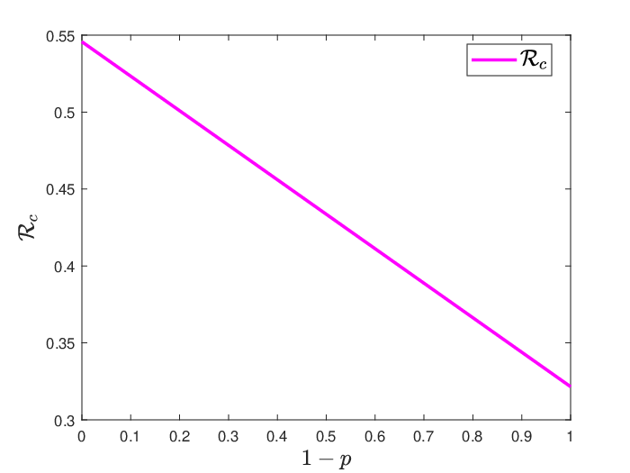
Now, we analyze the impact of asymptomatic transmission on COVID-19. Using the data of India in Tab. 2, we can observe that if $b\leq 0.28991$ , then $\mathcal{R}_{c}$ is negatively correlated with $1-p$ as shown in Fig. 12, while in case of $b>0.28991$ , $\mathcal{R}_{c}$ is positively correlated with $1-p$ as shown in Fig. 12. From Fig. 13, it can be seen intuitively that $\mathcal{R}_{c}$ can change from greater than 1 to less than 1 when both $1-p$ and $b$ are changed. This suggests that asymptomatic infections play a key role in the spread of COVID-19.

6.1.3 Sensitivity analysis

The sensitivity index [9] of $\mathcal{R}_{c}$ with respect to parameter $k$ is expressed as

\xi_{k}^{\mathcal{R}_{c}}=\frac{\partial\mathcal{R}_{c}}{\partial k}\cdot\frac{k}{\mathcal{R}_{c}}.

(17)

It can be seen from (3) that $\mathcal{R}_{c}$ is affected by the parameters $a$ , $\beta$ , $p$ , $c$ , $b$ , $d$ , $q_{1}$ , $q_{2}$ , $r_{1}$ , $r_{2}$ . The values of parameters $p$ , $c$ and $d$ are difficult to be changed by artificial measures, so that they are fixed in the spread of COVID-19. We will analyze the remaining seven parameters. According to (3) and (17), we can obtain

	$\displaystyle\xi_{a}^{\mathcal{R}_{c}}$	$\displaystyle=\frac{\beta}{c+d}\cdot\frac{a}{\mathcal{R}_{c}}=\frac{aB_{1}B_{2}}{aB_{1}B_{2}+pcB_{2}+bc(1-p)B_{1}},$
	$\displaystyle\xi_{\beta}^{\mathcal{R}_{c}}$	$\displaystyle=\left[\frac{a}{c+d}+\frac{pc}{(c+d)B_{1}}+\frac{bc(1-p)}{(c+d)B_{2}}\right]\cdot\frac{\beta}{\mathcal{R}_{c}}=1,$
	$\displaystyle\xi_{b}^{\mathcal{R}_{c}}$	$\displaystyle=\frac{\beta c(1-p)}{(c+d)B_{2}}\cdot\frac{b}{\mathcal{R}_{c}}=\frac{cb(1-p)B_{1}}{aB_{1}B_{2}+pcB_{2}+cb(1-p)B_{1}},$
	$\displaystyle\xi_{q_{1}}^{\mathcal{R}_{c}}$	$\displaystyle=-\frac{pc\beta}{(c+d)B_{1}^{2}}\cdot\frac{q_{1}}{\mathcal{R}_{c}}=-\frac{pcq_{1}B_{2}}{B_{1}\left[aB_{1}B_{2}+pcB_{2}+cb(1-p)B_{1}\right]},$
	$\displaystyle\xi_{q_{2}}^{\mathcal{R}_{c}}$	$\displaystyle=-\frac{bc\beta(1-p)}{(c+d)B_{2}^{2}}\cdot\frac{q_{2}}{\mathcal{R}_{c}}=-\frac{bc(1-p)q_{2}B_{1}}{B_{2}\left[aB_{1}B_{2}+pcB_{2}+cb(1-p)B_{1}\right]},$
	$\displaystyle\xi_{r_{1}}^{\mathcal{R}_{c}}$	$\displaystyle=-\frac{pc\beta}{(c+d)B_{1}^{2}}\cdot\frac{r_{1}}{\mathcal{R}_{c}}=-\frac{pcr_{1}B_{2}}{B_{1}\left[aB_{1}B_{2}+pcB_{2}+cb(1-p)B_{1}\right]},$
	$\displaystyle\xi_{r_{2}}^{\mathcal{R}_{c}}$	$\displaystyle=-\frac{bc\beta(1-p)}{(c+d)B_{2}^{2}}\cdot\frac{r_{2}}{\mathcal{R}_{c}}=-\frac{bc(1-p)r_{2}B_{1}}{B_{2}\left[aB_{1}B_{2}+pcB_{2}+cb(1-p)B_{1}\right]}.$

By substituting the data of India in Tab. 2, the sensitivity index can be obtained as shown in Tab. 4.

Table 4: Sensitivity index of

\mathcal{R}_{c}

with respect to parameters.

Parameter	Sensitivity index $\xi_{k}^{\mathcal{R}_{c}}$ of $\mathcal{R}_{c}$
$\beta$	+1
$b$	+0.5863
$q_{2}$	-0.3626
$r_{2}$	-0.2237
$a$	+0.1910
$q_{1}$	-0.1701
$r_{1}$	-0.0526

The control reproduction number $\mathcal{R}_{c}$ is the most sensitive to transmission rate $\beta$ and the least sensitive to recovery rate $r_{1}$ of symptomatic infections. Additionally, $\mathcal{R}_{c}$ is positively correlated with $a$ , $\beta$ , $b$ , and negatively correlated with $q_{1}$ , $q_{2}$ , $r_{1}$ , $r_{2}$ . Theoretically, the most effective measures to control COVID-19 in India are to increase the quarantine rate $q_{2}$ of asymptomatic infections, reduce the transmission rate $\beta$ and $b$ of infected individuals, and enhance the cure rate $r_{2}$ of asymptomatic infections.

6.2 Case study in short-term COVID-19 model

Nanjing Bureau of Statistics reported [26] on 24 May 2021 that population of Nanjing is $\mathcal{N}=9314685$ . We collected the number of daily new COVID-19 cases and cumulative confirmed COVID-19 cases from [25]. Furthermore, we collated and processed the data in [25] and we considered all patients with positive nucleic acid to be infected. Nanjing showed a sudden surge of daily new COVID-19 cases on July 25-27, 2021 since mass nucleic acid testing of Nanjing in the second round [24]. Consequently, to get good fitting parameter results, we selected the daily new case data after July 27, 2021, and estimated some parameter values of Nanjing, see Tab. 5.

Table 5: Parameter estimates of COVID-19 model (13).

Parameter	Parameter value of Nanjing	Source
$\beta$	$0.0020$	Estimated
$a$	0.0168	Estimated
$b$	0.0090	Estimated
$c$	$\frac{1}{5.2}$	[18]
$p$	0.8702	[12]
$q_{1}$	0.0757	Estimated
$q_{2}$	0.1701	Estimated
$r_{1}$	0.1621	Estimated
$r_{2}$	$\frac{1}{12.5}$	[22]
$r_{3}$	$\frac{1}{10}$	[31]
$S(0)$	$9.3144\times 10^{6}$	Estimated
$E(0)$	9.9246	Estimated
$I(0)$	$1.3604\times 10^{2}$	Estimated
$A(0)$	39.423	Estimated
$Q(0)$	71.140	Estimated
$R(0)$	9.7078	Estimated

The daily new cases and the final size in Nanjing were further fitted (blue part) and compared with the statistical data (red part) as shown in Figs. 15 and 15. The COVID-19 in Nanjing broke out on July 20, 2021 and disappeared on August 13, 2021.

As shown in Fig. 15, the statistical value of the final size is 235, while the ultimately fitted value is about 238, and the relative error is about $1.28\%$ , which indicates that our model is applicable.

The control reproduction number $\mathcal{R}_{c}$ in Nanjing can be calculated to be $0.0073<1$ . From Figs. 17 and 17, we can see that exposed individuals, symptomatically infected individuals, asymptomatically infected individuals and quarantined individuals will eventually tend to zero, which means that the COVID-19 will eventually disappear, see Theorems 5.1 and 5.3.

6.2.1 The impact of quarantine measures on COVID-19

From Fig. 18, we find that as the values of $q_{1}$ and $q_{2}$ increase, the value of $\mathcal{R}_{c}$ decreases. And it is more sensitive to change in $q_{1}$ than that of $q_{2}$ , which is consistent with our discussion in Section 6.2.3. Therefore, for COVID-19 in Nanjing at that time, strengthening quarantine measure of symptomatically infected individuals is more necessary.

In Figs. 20 and 22, the value of $q_{1}$ is changed while other parameters are fixed. We find that with the increase in $q_{1}$ , $I(t)$ tends to zero faster, as shown in Fig. 20, and the cumulative confirmed symptomatic infections also decrease (see Fig. 22). In Figs. 20 and 22, only the value of $q_{2}$ changes. As the value of $q_{2}$ increases, the time when $A(t)$ approaches zero is shorter and the cumulative number of asymptomatic infections shows a downward trend, as shown in Fig. 20 and Fig. 22, respectively. This suggests that the stronger the quarantine measures, the less harm COVID-19 will cause to human beings.

6.2.2 The impact of asymptomatic infections on COVID-19

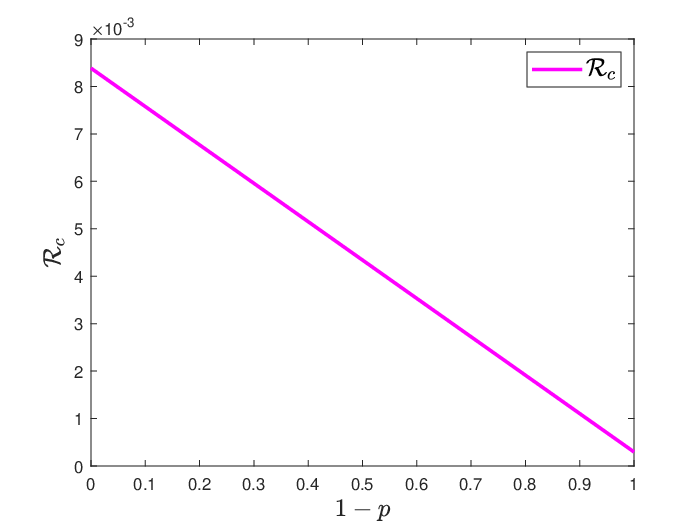
In the outbreak of COVID-19 in Nanjing, asymptomatic infections accounted for a small proportion of the total infections [25]. Nonetheless, asymptomatic transmission had played a non-negligible role in that outbreak. According to the data in Tab. 5, it can be calculated that the critical value of $b$ is about 1.0517. Hence, when $b\leq 1.0517$ , $\mathcal{R}_{c}$ is negatively correlated with $1-p$ , as shown in Fig. 24; when $b>1.0517$ , $\mathcal{R}_{c}$ is positively correlated with $1-p$ , as shown in Fig. 24. Meanwhile, Fig. 25 visually shows the effect of changes in $1-p$ and $b$ on $\mathcal{R}_{c}$ .

6.2.3 Sensitivity analysis

From (14) and (17), we can obtain the sensitivity index expressions of $\mathcal{R}_{c}$ with respect to seven parameters, respectively. The sensitivity index can be obtained by using the data in Tab. 5, as shown in Tab. 6. The parameters in the table are arranged from the most sensitive to the least sensitive.

	$\displaystyle\xi_{a}^{\mathcal{R}_{c}}$	$\displaystyle=\frac{\beta}{c}\cdot\frac{a}{\mathcal{R}_{c}}=\frac{a(q_{1}+r_{1})(q_{2}+r_{2})}{a(q_{1}+r_{1})(q_{2}+r_{2})+pc(q_{2}+r_{2})+bc(1-p)(q_{1}+r_{1})},$
	$\displaystyle\xi_{\beta}^{\mathcal{R}_{c}}$	$\displaystyle=\left(\frac{a}{c}+\frac{p}{q_{1}+r_{1}}+\frac{b(1-p)}{q_{2}+r_{2}}\right)\cdot\frac{\beta}{\mathcal{R}_{c}}=1,$
	$\displaystyle\xi_{b}^{\mathcal{R}_{c}}$	$\displaystyle=\frac{\beta(1-p)}{q_{2}+r_{2}}\cdot\frac{b}{\mathcal{R}_{c}}=\frac{cb(1-p)(q_{1}+r_{1})}{a(q_{1}+r_{1})(q_{2}+r_{2})+pc(q_{2}+r_{2})+cb(1-p)(q_{1}+r_{1})},$
	$\displaystyle\xi_{q_{1}}^{\mathcal{R}_{c}}$	$\displaystyle=-\frac{p\beta}{(q_{1}+r_{1})^{2}}\cdot\frac{q_{1}}{\mathcal{R}_{c}}=-\frac{pcq_{1}(q_{2}+r_{2})}{(q_{1}+r_{1})\left[a(q_{1}+r_{1})(q_{2}+r_{2})+pc(q_{2}+r_{2})+cb(1-p)(q_{1}+r_{1})\right]},$
	$\displaystyle\xi_{q_{2}}^{\mathcal{R}_{c}}$	$\displaystyle=-\frac{b\beta(1-p)}{(q_{2}+r_{2})^{2}}\cdot\frac{q_{2}}{\mathcal{R}_{c}}=-\frac{bc(1-p)q_{2}(q_{1}+r_{1})}{(q_{2}+r_{2})\left[a(q_{1}+r_{1})(q_{2}+r_{2})+pc(q_{2}+r_{2})+cb(1-p)(q_{1}+r_{1})\right]},$
	$\displaystyle\xi_{r_{1}}^{\mathcal{R}_{c}}$	$\displaystyle=-\frac{p\beta}{(q_{1}+r_{1})^{2}}\cdot\frac{r_{1}}{\mathcal{R}_{c}}=-\frac{pcr_{1}(q_{2}+r_{2})}{(q_{1}+r_{1})\left[a(q_{1}+r_{1})(q_{2}+r_{2})+pc(q_{2}+r_{2})+cb(1-p)(q_{1}+r_{1})\right]},$
	$\displaystyle\xi_{r_{2}}^{\mathcal{R}_{c}}$	$\displaystyle=-\frac{b\beta(1-p)}{(q_{2}+r_{2})^{2}}\cdot\frac{r_{2}}{\mathcal{R}_{c}}=-\frac{bc(1-p)r_{2}(q_{1}+r_{1})}{(q_{2}+r_{2})\left[a(q_{1}+r_{1})(q_{2}+r_{2})+pc(q_{2}+r_{2})+cb(1-p)(q_{1}+r_{1})\right]}.$

Table 6: Sensitivity index of

\mathcal{R}_{c}

with respect to parameters.

Parameter	Sensitivity index $\xi_{k}^{\mathcal{R}_{c}}$ of short-term model $\mathcal{R}_{c}$
$\beta$	+1
$r_{1}$	-0.6648
$q_{1}$	-0.3106
$a$	+0.0233
$b$	+0.0012
$q_{2}$	-0.0008
$r_{2}$	-0.0004

Similar to the conclusion in Tab. 4, the spread of the pandemic can be controlled by reducing transmission rates $a$ , $\beta$ , $b$ , strengthening quarantine measures $q_{1}$ , $q_{2}$ , and enhancing recovery rates $r_{1}$ , $r_{2}$ . The most effective measures for Nanjing were to reduce the transmission of symptomatically infected individuals and enhance the recovery rate of symptomatic infections and quarantine measures.

7 Conclusions

This paper not only analyzes the global stability of the COVID-19-free equilibrium $V^{0}$ and the COVID-19 equilibrium $V^{\ast}$ of model (1), but also solves the left problems in [16]. For the local stability of the COVID-19 equilibrium $V^{\ast}$ , it is difficult to use the Routh-Hurwitz criterion. To this end, we make use of proof by contradiction and the properties of complex modulus with some novel techniques and less computation. It is well known that the persistence result of model (1) is essential for the global attractivity of $V^{\ast}$ , and hence we prove weak persistence of model (1). To obtain the global stability results of $V^{0}$ and $V^{\ast}$ , we adopt the limit system of model (1) and Lyapunov function method. Specifically, $V^{0}$ is globally asymptotically stable for $\mathcal{R}_{c}<1$ and globally attractive for $\mathcal{R}_{c}=1$ in $\mathbb{R}_{+}^{6}$ , which implies that COVID-19 will disappear; $V^{\ast}$ is globally asymptotically stable for $\mathcal{R}_{c}>1$ in $\Omega$ , which indicates that COVID-19 will persist.

Although COVID-19 is in long-term development around the world since December 2019, COVID-19 disappeared in a short term on account of the strong prevention and control measures in some areas. For this reason, we propose a short-term COVID-19 model (13) based on model (1). It is sure that model (13) has no COVID-19 equilibrium. We work out the stability of the multiple COVID-19-free equilibria and the expression of the final size.

A retrospective study was conducted on the transmission of COVID-19 in India and Nanjing. We apply the long-term and the short-term models with publicly available official statistics to numerically demonstrate different transmission characteristics of COVID-19 in India and Nanjing, respectively. These numerical simulations validate the theoretical results of Theorems 4.1, 4.2, 5.1 and 5.3. The long-term model can well predict the spread of COVID-19 in India, and the short-term model perfectly fits the final size of Nanjing. Particularly, the relationship between the proportion of asymptomatic infected individuals and $\mathcal{R}_{c}$ is related to the transmission ability of asymptomatic infected individuals. As for India, case study shows that enhanced quarantine measures can not only prevent COVID-19 transmission but also reduce the peak value of infected individuals and cumulative confirmed cases. Asymptomatic transmission played a key role in the outbreak in India. For Nanjing, compared with asymptomatic infections, strengthening the quarantine measures for symptomatic infections is more conducive to controlling the spread of the COVID-19 at that time. With the strengthening of quarantine measures, infected individuals will tend to zero faster and the final COVID-19 size will decrease. It can be found that, although there are a few asymptomatic infections of the COVID-19 in Nanjing, the impact of asymptomatic transmission cannot be ignored, otherwise it will lead to inaccurate calculation of control reproduction number in Nanjing. As shown in Tabs. 4 and 6, the spread of COVID-19 can be reduced by vaccination, wearing masks, mass nucleic acid testing and strengthening quarantine measures, and so on. In addition, some measures to speed up the recovery rate of patients are also beneficial to control the COVID-19 pandemic.

Acknowledgements

This work is partially supported by the National NSF of China (Nos. 11901027, 11871093, 11671382, 11971273 and 12126426), the Major Program of the National NSF of China (No. 12090014), the State Key Program of the National NSF of China (No. 12031020), the NSF of Shandong Province (No. ZR2018MA004), and the China Postdoctoral Science Foundation (No. 2021M703426), the Pyramid Talent Training Project of BUCEA (No. JDYC20200327), and the BUCEA Post Graduate Innovation Project (No. PG2022143). The authors would like to thank Prof. Jing-An Cui and Dr. Liping Sun for their helpful suggestions.

References

[1] A. Alshorman, X. Wang, M. J. Meyer, et al., Analysis of HIV models with two time delays, J. Biol. Dynam., 11 (S1) (2017) 40–64.
[2] Y. Althobaity, J. Wu, M. J. Tildesley, A comparative analysis of epidemiological characteristics of MERS-CoV and SARS-CoV-2 in Saudi Arabia, Infect Dis. Model., 7 (3) (2022) 473–485.
[3] Y. Bai, X. Wang, S. Guo, Global stability of a mumps transmission model with quarantine measure, Acta Math. Appl. Sin.-E., 37 (4) (2021) 665–672.
[4] B. E. Bassey, J. U. Atsu, Global stability analysis of the role of multi-therapies and non-pharmaceutical treatment protocols for COVID-19 pandemic, Chaos Soliton. Fract., 143 (2020) 110574.
[5] S. Basu, R. P. Kumar, P. K. Santra, et al., Preventive control strategy on second wave of Covid-19 pandemic model incorporating lock-down effect, Alex. Eng. J., 61 (9) (2022) 7265–7276.
[6] S. C. Briand, M. Cinelli, T. Nguyen, et al., Infodemics: A new challenge for public health, Cell, 184 (25) (2021) 6010–6014.
[7] G. Butler, H. I. Freedman, P. Waltman, Uniformly persistent systems, Proc. Amer. Math. Soc., 96 (1986) 425–530.
[8] T. Chen, J. Rui, Q. Wang, et al., A mathematical model for simulating the phase-based transmissibility of a novel coronavirus, Infect. Dis. Poverty, 9 (1) (2020) 18–25.
[9] N. Chitnis, J. M. Hyman, J. M. Cushing, Determining important parameters in the spread of malaria through the sensitivity analysis of a mathematical model, Bull. Math. Biol., 70 (5) (2008) 1272–1296.
[10] J.-A. Cui, J. Lv, S. Guo, et al., Dynamical model of emerging infectious diseases–applied to COVID-19 transmission, Acta Math. Appl. Sin., 43 (2) (2020) 147–155. (in Chinese)
[11] P. van den Driessche, J. Watmough, Reproduction numbers and sub-threshold endemic equilibria for compartmental models of disease transmission, Math. Biosci., 180 (2002) 29–48.
[12] X. Gao, W. Chen, L. Guo, et al., Asymptomatic infection of COVID-19 and its challenge to epidemic prevention and control , Chin. J. Epidemiol., 41 (12) (2020) 1985–1988. (in Chinese)
[13] G. Giordano, F. Blanchini, R. Bruno, et al., Modelling the COVID-19 epidemic and implementation of population-wide interventions in Italy, Nat. Med., 26 (6) (2020) 855–860.
[14] S. Guo, W. Ma, Global behavior for delay differential equations model of HIV infection with apoptosis, Discrete Contin. Dyn. Syst.-Ser. B, 21 (1) (2016) 103–119.
[15] S. Guo, W. Ma, Remarks on a variant of Lyapunov-LaSalle theorem, Math. Biosci. Eng., 16(2) (2019) 1056–1066.
[16] S. Guo, Y. Xue, X. Li, Z. Zheng, A novel analysis approach of uniform persistence for a COVID-19 model with quarantine and standard incidence rate, arXiv:2205.15560, 2022.
[17] A. A. Kamara, L. N. Mouanguissa, G. O. Barasa, Mathematical modelling of the COVID-19 pandemic with demographic effects, J. Egypt. Math. Soc., 29 (2021) 8.
[18] Q. Li, X. Guan, P. Wu, et al., Early transmission dynamics in Wuhan, China, of novel coronavirus-infected pneumonia, N. Engl. J. Med., 382 (2020) 1199–1207.
[19] X.-X. Liu, S. J. Fong, N. Dey, et al., A new SEAIRD pandemic prediction model with clinical and epidemiological data analysis on COVID-19 outbreak, Appl. Intell., 51 (7) (2021) 4162–4198.
[20] J. Lv, S. Guo, J.-A. Cui, et al., Asymptomatic transmission shifts epidemic dynamics, Math. Biosci. Eng., 18 (1) (2020) 92–111.
[21] H. McCallum, N. Barlow, J. Hone, How should pathogen transmission be modelled?, Trends Ecol. Evol., 16 (6) (2001) 295–300.
[22] W.-K. Ming, J. Huang, C. J. P. Zhang, Breaking down of the healthcare system: Mathematical modelling for controlling the novel coronavirus (2019-nCoV) outbreak in Wuhan, China, Doi: 10.1101/2020.01.27.922443, 2020.
[23] B. Mizrahi, S. Shilo, H. Rossman, et al., Longitudinal symptom dynamics of COVID-19 infection, Nat. Commun., 11 (1) (2020) 6208.
[24] Nanjing Municipal Health Commission, Notice on carrying out the second round of nucleic acid testing for Nanjing city (No.5), http://wjw.nanjing.gov.cn/njswshjhsywyh/202107/t20210725_3084394.html, 25 July 2021. (in Chinese)
[25] Nanjing Municipal Health Commission, The latest situation of COVID-19 in Nanjing from 0:00 to 24:00 on 21 August, http://wjw.nanjing.gov.cn/njswshjhsywyh/202108/t20210822_3108683.html, 22 August 2021. (in Chinese)
[26] Nanjing Bureau of Statistics, Communiqué of the Seventh National Population Census of Nanjing, http://tjj.nanjing.gov.cn/njstjj/202105/t20210524_2945781.html, 24 May 2021. (in Chinese)
[27] Z. M. Nia, A. Ahmadi, N. L. Bragazzi, et al., A cross-country analysis of macroeconomic responses to COVID-19 pandemic using Twitter sentiments, PLoS One., 17 (8) (2022) e0272208.
[28] W. C. Roda, M. B. Varughese, D. L. Han, et al., Why is it difficult to accurately predict the COVID-19 epidemic?, Infect Dis. Model., 5 (2020) 271–281.
[29] S. Ruan, Likelihood of survival of coronavirus disease 2019, Lancet Infect. Dis., 20 (6) (2020) 630–631.
[30] A. M. Salman, I. Ahmed, M. H. Mohd, et al., Scenario analysis of COVID-19 transmission dynamics in Malaysia with the possibility of reinfection and limited medical resources scenarios, Comput. Biol. Med., 133 (2021) 104372.
[31] P. Shao, Y. Shan, Beware of asymptomatic transmission: Study on 2019-nCoV prevention and control measures based on extended SEIR model, Doi: 10.1101/2020.01.28.923169, 2020.
[32] B. Tang, W. Zhou, X. Wang, et al., Controlling Multiple COVID-19 Epidemic Waves: An Insight from a Multi-scale Model Linking the Behaviour Change Dynamics to the Disease Transmission Dynamics, Bull. Math. Biol., 84 (10) (2022) 106.
[33] H.R. Thieme, Convergence results and a Poincaré-Bendixson trichotomy for asymptotically autonomous differential equations, J. Math. Biol. 30 (7) (1992) 755–763.
[34] World Health Organization, Transmission of SARS-CoV-2: implications for infection prevention precautions: scientific brief, https://www.who.int/news-room/commentaries/detail/ transmission-of-sars-cov-2-implications-for-infection-prevention-precautions, 9 July 2020.
[35] World Health Organization, Considerations for implementing and adjusting public health and social measures in the context of COVID-19, https://apps.who.int/iris/rest/bitstreams/1351572/retrieve, 14 June 2021.
[36] World Health Organization, WHO coronavirus (COVID-19) dashboard, https://covid19.who.int, 31 October 2022.
[37] Worldometer, Coronavirus, https://www.worldometers.info/coronavirus/country/india, 26 September 2022.
[38] X. Xu, P. Chen, J. Wang, et al., Evolution of the novel coronavirus from the ongoing Wuhan outbreak and modeling of its spike protein for risk of human transmission, Sci. China Life Sci., 63 (3) (2020) 457–460.
[39] P. Yuan, E. Aruffo, Y. Tan, et al., Projections of the transmission of the Omicron variant for Toronto, Ontario, and Canada using surveillance data following recent changes in testing policies. Infect Dis. Model., 7 (2) (2022) 83–93.
[40] R. Yuan, Y. Ma, C. Shen, et al., Global dynamics of COVID-19 epidemic model with recessive infection and isolation, Math. Biosci. Eng., 18 (2) (2021) 1833–1844.
[41] M. Zamir, K. Shah, F. Nadeem, et al., Threshold conditions for global stability of disease free state of COVID-19, Results Phys., 21 (2021) 103784.
[42] X. Zhang, Y. Song, S. Tang, et al., Models to assess imported cases on the rebound of COVID-19 and design a long-term border control strategy in Heilongjiang Province, China, Math. Biosci. Eng., 19 (1) (2022) 1–33.

Dynamics of COVID-19 models with asymptomatic infections and quarantine measures

Abstract

Keywords:

2020 MSC

1 Introduction

2 Local stability of the COVID-19 equilibrium

Theorem 2.1.

Proof.

3 Weak persistence

Lemma 3.1.

Proof.

Lemma 3.1′.

Proof.

Theorem 3.1.

Proof.

Corollary 3.1.

4 Global stability

Theorem 4.1.

Proof.

Theorem 4.2.

Proof.

5 Dynamics of short-term COVID-19 model

5.1 Stability analysis

Theorem 5.1.

Proof.

Theorem 5.2.

Proof.

Theorem 5.3.

Proof.

5.2 The final COVID-19 size

6 Case study

6.1 Case study in long-term COVID-19 model

6.1.1 The impact of quarantine measures on COVID-19

6.1.2 The impact of asymptomatic infections on COVID-19

6.1.3 Sensitivity analysis

6.2 Case study in short-term COVID-19 model

6.2.1 The impact of quarantine measures on COVID-19

6.2.2 The impact of asymptomatic infections on COVID-19

6.2.3 Sensitivity analysis

7 Conclusions

Acknowledgements

References

References

Lemma 3.1^′.