Prototypical few-shot segmentation for cross-institution male pelvic structures with spatial registrationJournal: Medical Image Analysis
Abstract
The prowess that makes few-shot learning desirable in medical image analysis is the efficient use of the support image data, which are labelled to classify or segment new classes, a task that otherwise requires substantially more training images and expert annotations. This work describes a fully 3D prototypical few-shot segmentation algorithm, such that the trained networks can be effectively adapted to clinically interesting structures that are absent in training, using only a few labelled images from a different institute. First, to compensate for the widely recognised spatial variability between institutions in episodic adaptation of novel classes, a novel spatial registration mechanism is integrated into prototypical learning, consisting of a segmentation head and an spatial alignment module. Second, to assist the training with observed imperfect alignment, support mask conditioning module is proposed to further utilise the annotation available from the support images. Extensive experiments are presented in an application of segmenting eight anatomical structures important for interventional planning, using a data set of 589 pelvic T2-weighted MR images, acquired at seven institutes. The results demonstrate the efficacy in each of the 3D formulation, the spatial registration, and the support mask conditioning, all of which made positive contributions independently or collectively. Compared with the previously proposed 2D alternatives, the few-shot segmentation performance was improved with statistical significance, regardless whether the support data come from the same or different institutes.
Keywords:
\KWDfew-shot learning, multi-class segmentation, image registration, pelvic MRI1 Introduction
Multi-structure segmentation is one of the fundamental computing tasks in medical imaging applications, found in diagnosis, treatment, and monitoring, and remains a research interest. Diagnosis of varieties of diseases can be assisted by quantifying the morphology, or its change, of multiple structures. For example, brain disorders, including Alzheimer’s disease [34] and Parkinson [21], associates with abnormal volumes or shapes of neurological regions. Identifying brain structures is the key to many quantitative studies, such as functional activation mapping and brain development analysis [14]. Minimally invasive treatments often benefit from careful planning of both interventional instruments and guidance imaging, with respect to segmented patient-specific anatomical structures. In endoscopic pancreatobiliary procedures, as previously reported, image guidance that displays registered anatomical models outside the endoscopic field of view helps the surgeon during targeting and navigation [18].
This work is primarily concerned with segmenting multiple organs and urologically interesting structures on T2-weighted MR images from prostate cancer patients, to plan targeted biopsy, focal therapy, and, increasingly, other therapeutic procedures such as radiotherapy. Accurate segmentation of these structures help with targeting suspected cancerous regions found in multiparametric MR imaging with respect to the prostate gland and avoiding vulnerable surrounding structures, such as rectum, bladder and neurovascular bundles, for minimising risks in infection, impotence and other potential injury and complications [37].
The data-driven representation learning enabled by deep neural networks has led to promising segmentation results in multi-structure segmentation tasks, for example, in neuroimaging [16] and abdominal organs [49]. Automating this task reduces the current requirement of manual segmentation which is often associated with costs in expertise and intra- and inter-observer variations [9]. However, recent supervised segmentation methods mostly rely on large data sets with full annotations, subject to the similar limitations in labelling, albeit only with training. On the other hand, few-shot image learning aims to classify unseen classes using only a few labelled examples [41, 44]. For medical image segmentation, such novel classes may represent new types of organ or anatomical regions, whose expert annotations are not available for large training data sets. Using our intended interventional planning application as an example, different biopsy or therapy procedures may require different anatomical structures and pathological regions to be annotated during the planning stage. Prostate zonal structures, if not routinely segmented for MR-planning of radiotherapy, may provide more precise target localisation in registration-assisted ultrasound-guided focal ablation or a new therapy.
The now well-recognised performance loss in cross-institute generalisation of deep learning models [11] has motivated a body of research such as domain adaptation [35, 30] and federated learning [24]. This work focuses on few-shot segmentation with the practically important cross-institution context (as shown in Fig. 1), which aims to segment a novel class from a query image, given only a few support images and their binary masks of the novel class, from a novel institution where the limited labelled data are available. In other words, the model should be able to simultaneously adapt to both novel classes and novel institutions.
To improve the inter-class and inter-institute generalisation, this work first examines the manifestation of the performance-reducing inter-institute variability in prototypical few-shot image segmentation algorithms. In particular, we investigate the impact of spatial alignment, or the lack thereof, between support and query data from different institutes, a key component in such prototypical learning paradigm, on the few-shot segmentation accuracy.
First, addressing one of the previously identified challenges of spatial inconsistency [46], also found in medical image applications [12, 43], we develop a spatial registration mechanism to align the support and query images prior to the comparison between the two. This spatial registration mechanism consists of a segmentation head and a spatial alignment module, trained end-to-end, and is motivated by medical-image-specific observations of the difference between intra- and inter-institution data characteristics, due to different scanners and local imaging protocols, discussed further in Section 4.4.
Second, we propose an additional support mask conditioning module, also trained end-to-end, to enforce the conditioning on the available novel class labels. The conditioning module is empirically designed to work together with the spatial registration mechanism, to maximise utilisation of the few and prized support masks.
In addition to the evaluation of efficacy due to each proposed component, this work also demonstrates the benefit of the proposed 3D formulation, replacing existing 2D neural network-based few-shot segmentation approaches [8, 32, 38, 1, 12, 45, 52, 43].
One widely identified problem in both developing and evaluating multi-structure segmentation algorithms is the lack of a sizable labelled data set. To the date of submission of this paper, there were no multi-structure annotations publicly available for pelvic MR images. Through this work, all of our manual labels from open data sets have been made available at https://zenodo.org/record/7013610, for aiding the reproducibility of this work and, potentially, for other urologic or radiologic tasks concerning multiple pelvic anatomical structures.
Our preliminary results were recently presented [26], contributions from this paper include 1) a more detailed description and discussion of the spatial registration mechanism, 2) a new support mask conditioning module, 3) a substantially larger and fully labelled data set, and 4) more ablation comparison experiments. These are also summarised as follows.
- 1.
We introduced the cross-institution few-shot segmentation task to address the data scarcity problem specifically faced in medical applications.
- 2.
We first proposed to extend prototypical neural network to 3D for few-shot multi-class segmentation, which requires fewer parameters while achieving similar performance to its 2D counterpart.
- 3.
We developed an spatial registration mechanism and a support mask conditioning module, directly addressing the observed limitations in medical image few-shot segmentation, for improving generalisation across data from different institutions.
- 4.
We presented extensive ablation studies to investigate the impact of the proposed individual components, the increasing number of support data, the varying size of the training set, and the permutations in the available institutes.
- 5.
We published all expert annotations based on public image data sets at https://zenodo.org/record/7013610, which includes full segmentation of eight distinctive male lower pelvic structures on 589 3D MR images (including 178 3D MR images from our preliminary work [26]).
- 6.
The code implementing the proposed algorithms has also been made publicly available at https://github.com/kate-sann5100/CrossInstitutionFewShotSegmentation.
2 Related Work
2.1 Few-shot segmentation
The few-shot segmentation task was first introduced in computer vision applications [39] where the goal is to segment the novel class in a query image in the presence of a few support images having the same class labelled. Using episodic training which takes both query and support images as input, [39] demonstrated a better performance compared to the common fine-tuning methods, which fine-tunes the models on the support images per novel class. In 2018, Dong and Xing 2018 proposed prototypical episode learning that represents the novel class in the support image with a single prototype vector and compares it with query features to perform segmentation. This strategy was later adopted in many further research works [53, 29, 25].
Due to the common challenges in data collection, few-shot segmentation was also adapted to different medical images, including CT [38], MRI [31], ultrasound [12], etc. The early methods applied fine-tuning strategy and addressed the over-fitting on support images with multi-tasking [31, 5] and data augmentation [54, 15, 48]. Roy et al. 2020 was one of the first that adopted prototypical learning in medical imaging, reporting promising performance. [32] and [52] extracted multiple prototype vectors and performed a location-guided comparison, with the assumption of similar spatial layouts between the query and support images. However, in cross-institution scenarios, regions of interest may be located differently between queries and supports, as shown in Fig. 9. In this work, we proposed an integrated spatial registration mechanism to address such inconsistency.
In addition to data scarcity, higher-dimensional data in medical imaging often poses practical challenges in neural network training. Roy et al. 2020 proposed to use 2D neural networks, that pre-trained on large data sets such as ImageNet, and performed slice-by-slice inference when applied to 3D medical images. This strategy was also adopted by most of the follow-up prototypical methods [8, 32, 1, 12, 45, 52, 43]. Kim et al. 2021 integrated a bidirectional gated recurrent unit to process 2D features extracted from adjacent slices. Zhou et al. 2021 proposed 3D pyramid reasoning modules (PRMs) to model the anatomical correlation between query features at each location and all support features at neighbouring corresponding locations. To reduce computational cost, a relatively small number of channels were used for each convolutional kernel. The proposed method, in contrast, reduced the number of comparisons by extracting a single prototype vector for each spatial window.
To the best of our knowledge, there has been no prior work that successfully deployed 3D neural networks that receive and output 3D image volumes directly, using prototypical training for few-shot segmentation in medical imaging applications. Investigating the 3D formulation is not only technically interesting, but may also lead to potentially superior performance and/or efficiency in this inherently 3D segmentation task.
2.2 Cross-institution learning
The proposed cross-institution few-shot segmentation task aims to segment a novel class in images from a novel institution, with support images and labels from the same novel or other non-novel institutions. Although the objective is also to generalise on novel data, it differs from federated learning and domain adaptation due to their constraints on data privacy, accessibility, and availability. However, an optimal gain in efficient use of labelled data could be achieved by combining these methods with few-shot learning.
Federated learning is a learning paradigm that targets the problem of data governance and privacy by training algorithms collaboratively without the need for physically exchanging the data themselves, sometimes requiring the compliance of varying access policy [36]. It has been used in different medical imaging applications [24], but the focus is mainly on improving performance in trained classes without the need for generalisation in a novel class.
There exist three different domain adaptation methods: supervised, unsupervised, and semi-supervised. While sharing the same overarching objective, i.e. generalising to new domains such as novel classes, the supervised domain adaptation [17] does not explicitly focus on the data scarcity as few-shot learning. Unsupervised methods [33], on the other hand, often assume large-scale data set from the novel institution but without labels, thus paying a different attention from that of cross-institution few-shot learning. Combining both techniques, semi-supervised methods [10, 50] can leverage labelled and unlabelled data sets more efficiently.
Despite the distinct focuses, techniques and methodologies from federated learning and domain adaptation have indeed been considered in developing our cross-institute few-shot segmentation approach. For example, the spatial normalisation and divergence between features have commonly been adopted in federated learning [23] and feature-level domain adaptation [47], respectively.

3 The Cross-Institution Few-Shot Segmentation Task
Consider a set of classes and institutions, and , respectively. For each institution , denotes the set of all images. All classes have been segmented for each image: given a class , represents the corresponding mask for the image from the institution .
The classes and the institutions are split into disjoint sets and , respectively. The images of each institution are also separated into disjoint training and test subsets and . A base data set is formed with training images and the corresponding labels of the base classes from all the base institutions.
| (1) |
Similarly, test images and the corresponding labels of novel classes from all base institutions form another data set,
| (2) |
together with the data set of images from the novel institutions and the novel classes’ labels,
| (3) |
a novel data set is built focusing on novel classes:
| (4) |
Therefore, the cross-institution segmentation task aims to train a model on the base data set and generalise to the novel data set which contains novel classes on both base and novel institutions. Specifically, following the few-shot setting described in [38] and [32], the model is tasked to segment a novel class in a query image acquired from a novel institution with only support examples from the same or different institutions. The predicted query mask is compared with the label with a segmentation metric such as the Dice score [42]. Such evaluation procedure is named an episode with -shot, which is also detailed in Algorithm 1.
for do
for do
Denote the mask of in as
Predict
Evaluate
Update
Update
Update
Update
end for
for do
Denote the mask of in as
Predict
Evaluate
Update
Update
Update
Update
end for
Compute
Compute
4 Method
4.1 Episodic Few-shot Training
This work adopts the common episodic training paradigm (detailed in Algorithm 2) that simulates the few-shot task during training. Each episode consists of query and support image-label pairs, for a base class sampled from . In this work, during training and the model is trained to predict the query mask given the query image and one support image-label pair, denoted as .
Sample , such that
Denote the mask of in as
Denote the mask of in as
Predict
Compute loss:
Update model parameters: end while
4.2 Prototypical Network
A prototypical network [7] first defines a prototype feature vector per class, extracted from the embedded features of the labelled voxels, in the support image, corresponding to the class. The feature vector is then compared with the query image voxel-wise in the embedded feature space for segmentation prediction.
Specifically, the query and support images, denoted by and respectively, are encoded by a shared feature extractor into support and query feature maps of the same shape, and , respectively. The class prototype and the background prototype are then derived by averaging over voxels of the class (where label equals ) and background (where label equals ), respectively, i.e., and , where
| (5) |
with iterating over all voxels in along x, y and z axes.
The similarity between each query voxel and class (or background) is calculated through cosine similarity between the voxel feature map and the class prototype feature vector (or for background):
| (6) |
where represents the class or background, and represents the dot product between vectors.
4.3 Local Prototypical Network
To extract location-sensitive local prototypes [52], images of spatial size are partitioned into overlapping windows of size with the equidistant spacing between window centres being half of the window size. As shown in Fig. 2, for each window , two local prototype feature vectors and are calculated via Eq. (5) by iterating over the voxels inside the window : and , where
| (7) |
For each query voxel , denotes the set of all windows that contains the voxel: . The local similarity between this voxel and the class (or background) is then calculated using the maximum cosine similarity over windows with the corresponding local prototype feature vectors and :
| (8) |
with representing the class or background. The foreground/background probability map is derived by:
| (9) |
with representing the class and background. The model is trained to minimise the Dice loss between the predicted and ground-truth mask:
| (10) |
where
4.4 Spatial Registration Mechanism

As discussed in Section 1, the differences in intra- and inter-institution variations pose challenges in the local prototypical network due to the varying image sizes, orientations, and voxel dimensions of the acquiring institution. The target structure in the query and support images can be distant (as in Fig. 9). Therefore, they may not be included inside of the same or even adjacent windows, and this results in erroneous comparison between the query voxels of the structure, thus irrelevant prototype vectors. However, while the absolute locations of target structures varies among images, the relative position between different structures remains consistent. This observation motivated spatial alignment of the query and the support images, and , illustrated in Fig. 2, before extracting the local prototype feature vectors. This spatial registration process is conjectured to alleviate the discrepancy between different institutions and therefore reduce the amount of cross-institution training data required for generalisation.
In this work, we consider an affine transformation to account for the above-discussed spatial difference with potentially uncertainties due to variable imaging positioning, signal sampling and scanner calibration, although higher-degree transformation will also be of interest. Furthermore, to avoid repeated feature map extraction, we propose to apply the transformation directly on feature maps ( and ), rather than on images ( and ).
The affine transformation prediction consists of two stages. Firstly, a shared base class segmentation head segments all base classes from the query and support feature maps, and , respectively. The multi-class predictions are denoted as and , for the query and support images, respectively. During evaluation, these predictions are concatenated and passed into the spatial alignment module, illustrated in Fig. 2, which predicts an affine transformation matrix of degrees of freedom. During training, as illustrated in Fig. 3, base classes segmentation masks and are used for alignment prediction. Secondly, alignment is applied to the support feature map and the label , to obtain the aligned support feature map and the aligned support label for all base classes , respectively. These aligned feature maps are then used to generate the local prototypes (as detailed in Section 4.3) for segmentation.
Two losses are defined for training the spatial registration mechanism. First, a Dice loss is defined for the multi-class segmentation:
| (11) |
where the multi-class Dice loss is defined as:
| (12) |
with and representing the ground truth and the predicted probability of a base class or background at .
The second loss aims to optimise alignment by minimising the Dice loss between the query label and the aligned support label of all base classes:
| (13) |
In theory, the transformation could be applied the other way around, i.e. by applying the reverse alignment to the query feature map resulting in the aligned query feature map , to achieve spatial alignment between query and support features. A cycle-consistent two-way registration may also apply. However, once the aligned query mask is predicted, it needs to be inverted, in order to obtain the mask of the original query image . The mechanism was adopted in this work for its computational efficiency without additional resampling in practice.
4.5 Support Mask Conditioning Module
During the prototype feature vector extraction using the novel class mask in the support image, the voxel-wise information may be made invariant to the transformation during the aggregation in Eq. (5) and (7), which is designed for “normalising” cross-institution data, but may also result in large spatial variability in the prediction. Therefore, a simple yet effective support mask conditioning module is proposed.
The support mask conditioning module takes as input a concatenation of the class similarity , the background similarity and the aligned mask of the class in the support image , for the final prediction . Unlike the multiplication of support mask to support features for prototype calculation (in Eq. (5) and (7)), the direct use of support mask here provides a more direct route for the novel class information to the final segmentation task, similar to commonly designed shortcut layers for skipping networks.
Different from 3D medical segmentation algorithms using mask predicted from downsampled image to provide context information for high-resolution patches, the proposed method uses the segmentation of query image with location and shape information of the support mask.
4.6 Loss
Both the spatial registration mechanism and support mask conditioning module are trained with the original local prototypical network, with an overall training loss function used in this study as follows:
| (14) |
4.7 Multiple-shot Evaluation
Due to memory limitation, the training was carried out in one-shot paradigm, i.e. . During the evaluation, for the query image and each of the support images , the base class segmentation is predicted from the base class segmentation head, denoted by and , respectively. Among the support images, only the support image that is the most similar to the query image in terms of the cosine similarity on base class segmentation prediction, denoted by , is chosen to calculate the local prototypes in (7). Precisely,
| (15) |
where the dot product and norm are calculated on the flattened predictions. The local prototypes are then calculated using the selected support example, and for each window .
5 Experiments
5.1 Data Set
| institution | ||||||||
|---|---|---|---|---|---|---|---|---|
| 1 | 2 | 3 | 4 | 5 | 6 | 7 | total | |
| # of images | 321 | 45 | 74 | 82 | 24 | 24 | 19 | 589 |
The data set includes 589 T2-weighted images acquired from the same number of patients collected by seven studies, INDEX [6], the SmartTarget Biopsy Trial [13], PICTURE [40], TCIA Prostate3T [27], Promise12 [28], TCIA ProstateDx (Diagnosis) [2] and the Prostate MR Image Database [4]. Further details are reported in the respective study references.
These images were divided into seven subsets based on the acquiring institution. The number of images acquired from each institution is anonymously summarised in Table 1. The cross-institution imaging protocols contain multiple scanners (two manufacturers with a mixed 1.5 and 3T field strengths), varying field-of-view and anisotropic voxels, in-plane voxel dimensions ranging between 0.3 and 1.0 mm and out-of-plane spacing between 1.8 and 5.4 mm.
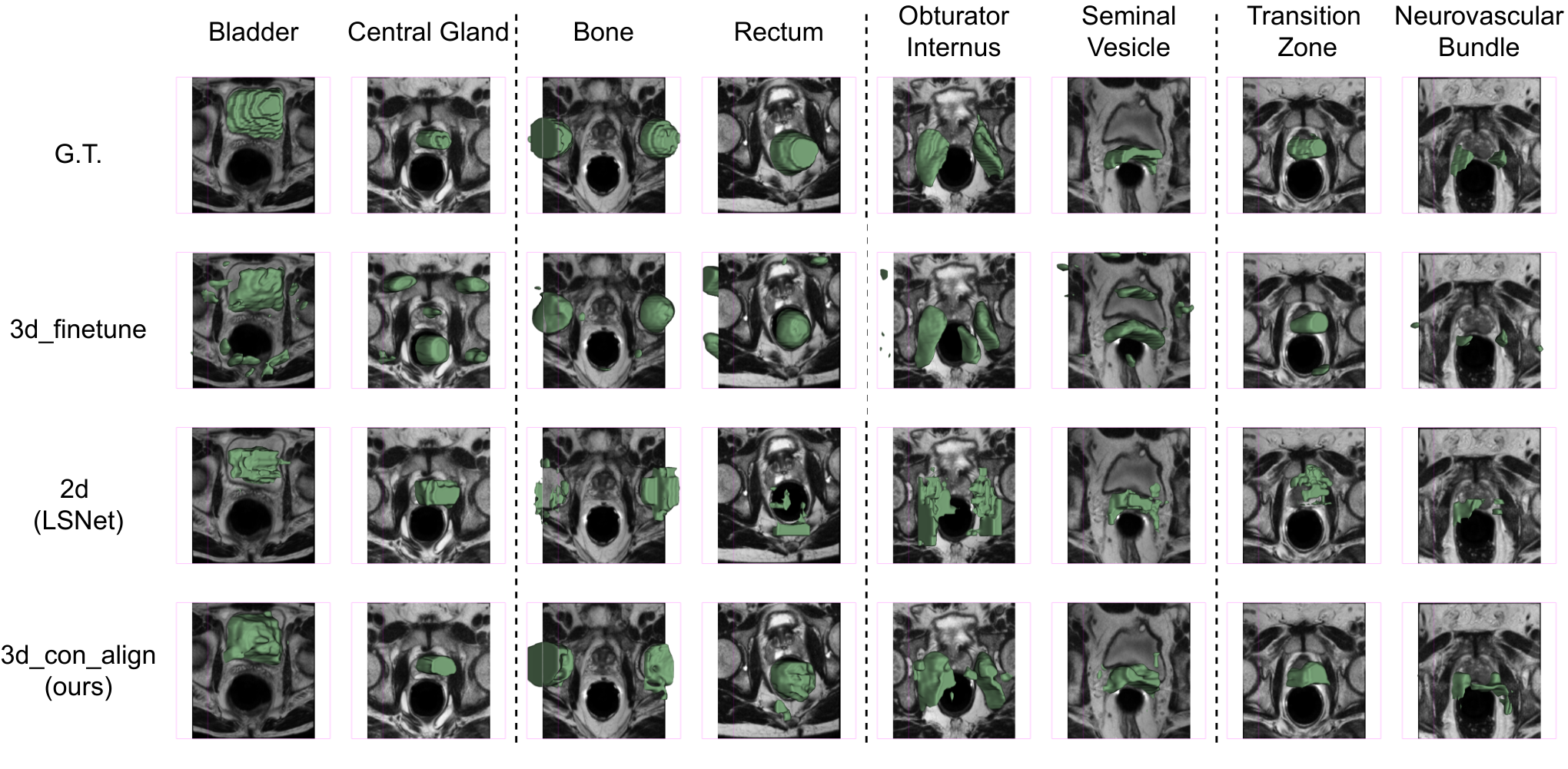
For each image, eight anatomical structures of planning interest, including bladder, bone, central gland, neurovascular bundle, obturator internus, rectum, seminal vesicle, transition zone were labelled (as shown in Fig.4). All segmentations were manually annotated by eight biomedical imaging researchers, with experience ranging from 2 to 10 years in the annotation of medical image data, each annotating a mixed-institution subset using an institution-stratified sampling. Each annotation has been reviewed at least once.
The full segmentation masks and the derived intensity arrays from T2-weighted sequences, after pre-processing, used to produce the results in this study, are available at https://zenodo.org/record/7013610.
The eight lower-pelvic structures were randomly divided into four folds as shown in Table 2. In a cross-validation experiment, the classes contained in each fold were considered as novel classes, the other three folds representing base classes. The images of each institution were then randomly sampled into training and testing subsets in a 3:1 ratio. A further validation set was formed with 12 images, 2 from each institution, randomly chosen from the novel data set . Those images were excluded from the testing. Unless otherwise specified, the same data partitioning was used for all the results presented. All statistical conclusions are reported using paired Student’s t-tests at the significance level of = 0.05.
| structures | |
|---|---|
| fold 1 | bladder, central gland |
| fold 2 | bone, rectum |
| fold 3 | obturator internus, seminal vesicle |
| fold 4 | transition zone, neurovascular bundle |
5.2 Implementation Details


All images were normalised, resampled and centre-cropped to an image size of , with a voxel dimension of during pre-processing. Random rotation, translation and scaling were adopted for data augmentation during training.
The best training episode was chosen based on the performance on the validation sets. During evaluation, all images from the novel institution were considered query images for evaluation for each of the fold-specified novel classes. A binary Dice score for this novel class was calculated for each query image based on a sampled support image from each of the seven institutions, excluding the query. As described in Algorithm 1, the results were reported when support images from 1) all institutions, 2) base institutions, and 3) novel institutions. The institution where the support image comes from is denoted as ‘support ins’.
A 3D UNet was adopted as the feature extractor, whose architecture is detailed in Fig. 5. and were selected for local prototypical comparison as detailed in Section 4.3. As shown in Fig. 6, the support mask conditioning module was made up of two convolutional layers. For the spatial registration mechanism, the base class segmentation head was a single convolutional layer, and the spatial alignment module was a GlobalNet [19] as specified in Fig. 7. The models were trained using an Adam optimiser starting at a learning rate of with a minibatch size of 1. The implementation code has been released at https://github.com/kate-sann5100/CrossInstitutionFewShotSegmentation.
5.3 Compared Baseline Networks
For comparison, we report the results of the following baseline networks.
- 1.
The ‘3d_finetune’ network - The ‘3d_finetune’ baseline implemented the same UNet as the feature extractor. It was pre-trained on the base data set to segment all base classes for epochs using an Adam optimiser starting at a learning rate of . During evaluation, for each query, the pre-trained model is fine-tuned on the support images for iterations before testing. This baseline provides a reference as a “lower-bound” performance, using a simple transfer learning strategy.
- 2.
The ‘2d’ network - LSNet [52] was adopted as the 2D episodic baseline. It adopted the same local-prototype comparison approach as detailed in Section 4.3 but using a 2D backbone based on ResNet-50 pre-trained on ImageNet, instead of 3D networks. To the best of our knowledge, this is the prototypical network closest to our work that has been proposed for medical image segmentation.
- 3.
BiGRU [22] - Another recent few-shot medical segmentation method with a UNet-like network for 2D slice prediction and a bidirectional gated recurrent unit (GRU) for adjacent slices consistency.
- 4.
The ‘localnet (unsupervised)’ network for multi-atlas segmentation - A non-rigid registration network, LocalNet [20], trained on the base data set images with no organ label supervision. Given a support-query pair, the model is trained to predict a dense displacement field that warps the support towards the query. For n-shot evaluation, dense displacement fields are predicted, each registering a support example towards the query. query mask predictions are derived by warping each support mask using the corresponding predicted dense displacement field. The final prediction is made through majority voting by the query mask predictions. The implementation was based on the open-source repository MONAI [3].
- 5.
The ‘localnet (supervised)’ network for multi-atlas segmentation - A non-rigid registration network, LocalNet [20], trained on the base data set with masks from all classes including novel classes. Similar to the ‘localnet(unsupervised)’ network, the query mask is the warped support mask using the registration-predicted support-to-query dense displacement field. The implementation was based on the open-source repository MONAI [3].
- 6.
The ‘3d_supervised’ network - A fully supervised 3D model was trained on the base data set images with masks from all classes. The results on the novel institution images are reported as an “upper-bound” performance.
| model | support | Dice (%) | 95% Hausdorff distance (mm) | #param | ||||||||
| ins | fold1 | fold2 | fold3 | fold4 | mean | fold1 | fold2 | fold3 | fold4 | mean | (million) | |
| 3d_finetune | all | 48.07 | 44.78 | 43.92 | 29.25 | 41.50 | 61.47 | 69.78 | 60.33 | 57.02 | 62.15 | 5.75 |
| base | 45.74 | 39.81 | 41.69 | 26.02 | 38.32 | 63.22 | 73.42 | 62.33 | 59.24 | 64.55 | ||
| novel | 62.03 | 74.56 | 57.31 | 48.63 | 60.63 | 50.98 | 47.96 | 48.32 | 43.72 | 47.74 | ||
| 26.26% | 46.60% | 27.25% | 46.48% | 36.80% | -24.02% | -53.09% | -28.99% | -35.51% | -35.21% | |||
| BiGRU | all | 44.05 | 43.08 | 29.61 | 20.97 | 34.43 | 23.70 | 33.67 | 23.60 | 22.83 | 25.95 | 38.85 |
| base | 44.05 | 42.74 | 29.21 | 20.62 | 34.15 | 23.73 | 34.06 | 23.85 | 23.20 | 26.21 | ||
| novel | 44.03 | 45.11 | 32.01 | 23.12 | 36.07 | 23.49 | 31.30 | 22.12 | 20.60 | 24.38 | ||
| -0.06% | 5.26% | 8.75% | 10.80% | 5.30% | -1.04% | -8.82% | -7.83% | -12.59% | -7.52% | |||
| 2d | all | 49.23 | 44.51 | 36.34 | 27.44 | 39.38 | 24.03 | 30.86 | 29.51 | 30.77 | 28.79 | 23.63 |
| base | 48.80 | 42.92 | 35.52 | 26.83 | 38.52 | 24.12 | 31.93 | 30.30 | 31.54 | 29.47 | ||
| novel | 51.80 | 54.07 | 41.28 | 31.08 | 44.56 | 23.52 | 24.39 | 24.83 | 26.13 | 24.72 | ||
| 5.80% | 20.62% | 13.94% | 13.68% | 13.55% | -2.54% | -30.92% | -22.03% | -20.72% | -19.24% | |||
| 3d | all | 47.79 | 52.06 | 34.81 | 26.16 | 40.20 | 31.60 | 30.68 | 32.95 | 31.71 | 31.73 | 5.75 |
| base | 47.89 | 51.07 | 34.12 | 25.44 | 39.63 | 31.69 | 31.03 | 33.35 | 32.19 | 32.07 | ||
| novel | 47.22 | 58.00 | 38.96 | 30.49 | 43.67 | 31.07 | 28.54 | 30.54 | 28.81 | 29.74 | ||
| -1.42% | 11.94% | 12.44% | 16.58% | 9.25% | -2.00% | -8.73% | -9.20% | -11.73% | -7.82% | |||
| 3d_con | all | 58.34 | 46.11 | 40.43 | 30.94 | 43.96 | 27.31 | 27.15 | 27.33 | 26.38 | 27.04 | 5.75 |
| base | 58.25 | 43.58 | 39.87 | 29.80 | 42.88 | 27.69 | 28.34 | 28.03 | 27.06 | 27.78 | ||
| novel | 58.84 | 61.30 | 43.81 | 37.78 | 50.43 | 25.04 | 20.02 | 23.14 | 22.30 | 22.63 | ||
| 1.00% | 28.91% | 8.99% | 21.12% | 14.98% | -10.56% | -41.54% | -21.12% | -21.31% | -22.76% | |||
| 3d_align | all | 50.80 | 51.56 | 32.39 | 30.89 | 41.41 | 27.33 | 36.29 | 32.63 | 29.93 | 31.55 | 27.34 |
| base | 50.60 | 51.17 | 31.25 | 30.82 | 40.96 | 27.35 | 36.82 | 33.01 | 30.42 | 31.90 | ||
| novel | 51.97 | 53.88 | 39.22 | 31.33 | 44.10 | 27.20 | 33.15 | 30.34 | 26.96 | 29.41 | ||
| 2.64% | 5.04% | 20.31% | 1.62% | 7.12% | -0.55% | -11.08% | -8.78% | -12.84% | -8.46% | |||
| 3d_con_align | all | 59.36 | 60.38 | 45.73 | 37.60 | 50.77 | 22.66 | 29.63 | 27.92 | 26.41 | 26.66 | 27.35 |
| base | 59.11 | 59.80 | 45.06 | 37.28 | 50.31 | 22.69 | 30.30 | 28.38 | 26.89 | 27.06 | ||
| novel | 60.86 | 63.87 | 49.77 | 39.54 | 53.51 | 22.49 | 25.63 | 25.19 | 23.54 | 24.21 | ||
| 2.89% | 6.37% | 9.47% | 5.70% | 5.98% | -0.91% | -18.21% | -12.65% | -14.26% | -11.79% | |||
| localnet | all | 25.64 | 38.99 | 21.83 | 11.20 | 24.42 | 28.74 | 27.21 | 24.78 | 26.97 | 26.93 | 5.94 |
| base | 24.16 | 36.43 | 21.03 | 10.35 | 22.99 | 29.43 | 28.48 | 25.39 | 27.89 | 27.80 | ||
| (unsupervised) | novel | 34.52 | 54.37 | 26.61 | 16.34 | 32.96 | 24.60 | 19.55 | 21.10 | 21.47 | 21.68 | |
| 30.01% | 33.00% | 20.98% | 36.67% | 30.25% | -19.63% | -45.70% | -20.32% | -29.93% | -28.22% | |||
| localnet | all | 72.70 | 72.14 | 52.84 | 42.65 | 60.08 | 19.36 | 22.81 | 21.78 | 24.00 | 21.99 | 5.94 |
| base | 71.80 | 70.11 | 51.21 | 41.65 | 58.69 | 20.29 | 24.69 | 23.07 | 25.11 | 23.29 | ||
| (supervised) | novel | 78.11 | 84.33 | 62.61 | 48.61 | 68.42 | 13.77 | 11.57 | 14.03 | 17.29 | 14.17 | |
| 8.09% | 16.86% | 18.20% | 14.31% | 14.21% | -47.33% | -113.31% | -64.37% | -45.26% | -64.39% | |||
| 3d_supervised | N/A | 89.01 | 91.68 | 81.44 | 70.30 | 83.11 | 4.73 | 5.14 | 5.91 | 6.83 | 5.65 | 5.75 |
| model | support | Dice (%) | 95% Hausdorff distance (mm) | ||||||||
|---|---|---|---|---|---|---|---|---|---|---|---|
| ins | fold1 | fold2 | fold3 | fold4 | mean | fold1 | fold2 | fold3 | fold4 | mean | |
| 3d_finetune | all | 37.61 | 29.23 | 33.06 | 20.25 | 30.04 | 59.83 | 71.87 | 50.66 | 51.62 | 58.49 |
| base | 36.72 | 28.33 | 31.11 | 20.02 | 29.05 | 60.77 | 73.85 | 52.09 | 52.02 | 59.68 | |
| novel | 42.96 | 34.63 | 44.73 | 21.63 | 35.99 | 54.16 | 59.97 | 42.09 | 49.20 | 51.36 | |
| 14.53% | 18.17% | 30.45% | 7.43% | 19.29% | -12.21% | -23.13% | -23.75% | -5.74% | -16.22% | ||
| 2d | all | 42.09 | 29.00 | 32.49 | 24.46 | 32.01 | 29.52 | 42.65 | 28.04 | 31.97 | 33.05 |
| base | 41.83 | 28.51 | 32.09 | 24.47 | 31.73 | 29.62 | 42.39 | 28.08 | 31.93 | 33.01 | |
| novel | 43.64 | 31.92 | 34.85 | 24.41 | 33.71 | 28.90 | 44.18 | 27.80 | 32.19 | 33.27 | |
| 4.14% | 10.68% | 7.92% | -0.26% | 5.87% | -2.50% | 4.05% | -1.00% | 0.80% | 0.79% | ||
| 3d_con_align | all | 57.58 | 37.42 | 37.42 | 30.18 | 40.65 | 23.02 | 37.56 | 30.22 | 28.52 | 29.83 |
| base | 57.71 | 36.74 | 36.70 | 29.97 | 40.28 | 22.90 | 38.37 | 30.74 | 28.52 | 30.13 | |
| novel | 56.83 | 41.46 | 41.70 | 31.40 | 42.85 | 23.75 | 32.72 | 27.12 | 28.51 | 28.02 | |
| -1.54% | 11.39% | 11.99% | 4.56% | 6.00% | 3.58% | -17.26% | -13.36% | -0.04% | -7.52% | ||
| 3d_supervised | N/A | 88.31 | 88.44 | 80.49 | 70.78 | 82.00 | 5.14 | 7.72 | 6.49 | 6.71 | 6.51 |
| model | support | Dice(%) | #param | ||||||
|---|---|---|---|---|---|---|---|---|---|
| ins | query institution | (million) | |||||||
| ins1 | ins2 | ins4 | ins5 | ins6 | ins7 | mean | |||
| BiGRU | same | 41.67 | 45.03 | 34.16 | 38.25 | 36.63 | 27.43 | 37.20 | 38.85 |
| diff | 35.40 | 34.00 | 31.60 | 34.09 | 36.77 | 25.76 | 32.94 | ||
| all | 36.18 | 35.38 | 31.92 | 34.61 | 36.75 | 25.97 | 33.47 | ||
| 15.06% | 24.49% | 7.49% | 10.88% | -0.37% | 6.09% | 11.45% | |||
| 2d | same | 48.41 | 49.15 | 39.00 | 53.49 | 44.33 | 34.52 | 44.82 | 23.63 |
| diff | 39.14 | 37.89 | 33.15 | 38.74 | 38.83 | 30.94 | 36.45 | ||
| all | 40.30 | 39.30 | 33.88 | 40.58 | 39.51 | 31.38 | 37.49 | ||
| 19.15% | 22.91% | 15.02% | 27.58% | 12.42% | 10.38% | 18.68% | |||
| 3d_con_align | same | 53.76 | 57.74 | 50.73 | 61.14 | 52.02 | 49.85 | 54.21 | 27.35 |
| diff | 49.55 | 50.39 | 47.64 | 53.73 | 51.38 | 46.22 | 49.82 | ||
| all | 50.08 | 51.30 | 48.03 | 54.65 | 51.46 | 46.67 | 50.37 | ||
| 7.83% | 12.73% | 6.08% | 12.12% | 1.23% | 7.29% | 8.10% | |||
| localnet | same | 36.42 | 48.05 | 27.66 | 39.53 | 26.51 | 19.94 | 33.02 | 5.94 |
| diff | 27.50 | 30.88 | 21.77 | 20.28 | 29.00 | 20.88 | 25.05 | ||
| (unsupervised) | all | 28.62 | 33.03 | 22.50 | 22.69 | 28.69 | 20.76 | 26.05 | |
| 24.49% | 35.73% | 21.30% | 48.69% | -9.37% | -4.68% | 24.13% | |||
| localnet | same | 73.05 | 64.65 | 41.41 | 73.38 | 68.87 | 40.44 | 60.30 | 5.94 |
| diff | 62.48 | 58.76 | 50.72 | 61.92 | 60.79 | 51.28 | 57.66 | ||
| (supervised) | all | 63.80 | 59.50 | 49.56 | 63.35 | 61.80 | 49.92 | 57.99 | |
| 14.47% | 9.11% | -22.49% | 15.62% | 11.74% | -26.81% | 4.38% | |||
| 3d_supervised | N/A | 86.77 | 84.08 | 80.75 | 86.36 | 80.16 | 80.69 | 83.14 | 5.75 |
baseline_2d_cross_ins.tex
2d
| s_ins | std | mean | p-value | ||||||||
|---|---|---|---|---|---|---|---|---|---|---|---|
| ins1 | ins2 | ins3 | ins4 | ins5 | ins6 | ins7 | |||||
| q_ins | ins1 | 53.76 | 53.31 | 50.63 | 46.46 | 50.77 | 47.78 | 47.83 | 2.62 | 50.08 | 1.06e-15 |
| ins2 | 54.26 | 57.74 | 50.07 | 44.42 | 51.97 | 52.05 | 48.62 | 3.91 | 51.30 | 0.08 | |
| ins3 | 51.11 | 50.17 | 53.51 | 49.41 | 52.25 | 47.25 | 51.67 | 1.90 | 50.77 | 2.04e-16 | |
| ins4 | 48.23 | 44.70 | 49.95 | 50.73 | 47.09 | 44.02 | 51.47 | 2.70 | 48.03 | 1.40e-05 | |
| ins5 | 54.70 | 52.88 | 54.38 | 54.14 | 61.14 | 50.56 | 54.77 | 2.98 | 54.65 | 0.15 | |
| ins6 | 52.10 | 55.89 | 51.69 | 44.23 | 52.70 | 52.02 | 51.61 | 3.26 | 51.46 | 9.47e-03 | |
| ins7 | 46.46 | 45.81 | 48.77 | 48.78 | 45.45 | 41.57 | 49.85 | 2.60 | 46.67 | 0.20 | |
| training | s_ins | Dice (%) | 95% Hausdorff distance (mm) | ||||||||
|---|---|---|---|---|---|---|---|---|---|---|---|
| data | fold1 | fold2 | fold3 | fold4 | mean | fold1 | fold2 | fold3 | fold4 | mean | |
| whole | all | 59.36 | 60.38 | 45.73 | 37.60 | 50.77 | 22.66 | 29.63 | 27.92 | 26.41 | 26.66 |
| base | 59.11 | 59.80 | 45.06 | 37.28 | 50.31 | 22.69 | 30.30 | 28.38 | 26.89 | 27.06 | |
| novel | 60.86 | 63.87 | 49.77 | 39.54 | 53.51 | 22.49 | 25.63 | 25.19 | 23.54 | 24.21 | |
| 2.89% | 6.37% | 9.47% | 5.70% | 5.98% | -0.91% | -18.21% | -12.65% | -14.26% | -11.79% | ||
| half | all | 55.38 | 57.16 | 42.54 | 34.14 | 47.30 | 25.98 | 29.37 | 31.65 | 29.00 | 29.00 |
| base | 55.08 | 55.49 | 41.82 | 33.75 | 46.54 | 26.04 | 30.13 | 32.17 | 29.37 | 29.43 | |
| novel | 57.16 | 67.17 | 46.88 | 36.46 | 51.91 | 25.56 | 24.81 | 28.52 | 26.84 | 26.43 | |
| 3.63% | 17.38% | 10.79% | 7.41% | 10.36% | -1.91% | -21.45% | -12.82% | -9.43% | -11.35% | ||
| half_single_ins | all | 52.85 | 57.46 | 31.31 | 20.39 | 40.50 | 26.84 | 29.38 | 35.41 | 33.89 | 31.38 |
| base | 52.17 | 56.06 | 30.55 | 19.63 | 39.60 | 26.93 | 29.93 | 36.04 | 34.41 | 31.83 | |
| novel | 56.90 | 65.87 | 35.85 | 24.93 | 45.89 | 26.29 | 26.10 | 31.65 | 30.75 | 28.70 | |
| 8.32% | 14.89% | 14.79% | 21.24% | 13.69% | -2.44% | -14.63% | -13.88% | -11.89% | -10.90% | ||
| quarter | all | 50.90 | 55.87 | 44.78 | 31.98 | 45.88 | 27.90 | 29.61 | 28.87 | 29.48 | 28.96 |
| base | 50.35 | 54.54 | 43.64 | 31.61 | 45.03 | 27.90 | 30.22 | 29.43 | 29.84 | 29.35 | |
| novel | 54.24 | 63.86 | 51.61 | 34.17 | 50.97 | 27.88 | 25.92 | 25.50 | 27.27 | 26.64 | |
| 7.17% | 14.60% | 15.45% | 7.49% | 11.65% | -0.05% | -16.60% | -15.41% | -9.43% | -10.15% | ||
| shot | # of shot | support | Dice (%) | 95% Hausdorff distance (mm) | ||||||||
|---|---|---|---|---|---|---|---|---|---|---|---|---|
| ins | fold1 | fold2 | fold3 | fold4 | mean | fold1 | fold2 | fold3 | fold4 | mean | ||
| 1 | 3d_finetune | all | 48.07 | 44.78 | 43.92 | 29.25 | 41.50 | 61.47 | 69.78 | 60.33 | 57.02 | 62.15 |
| base | 45.74 | 39.81 | 41.69 | 26.02 | 38.32 | 63.22 | 73.42 | 62.33 | 59.24 | 64.55 | ||
| novel | 62.03 | 74.56 | 57.31 | 48.63 | 60.63 | 50.98 | 47.96 | 48.32 | 43.72 | 47.74 | ||
| 26.26% | 46.60% | 27.25% | 46.48% | 36.80% | -24.02% | -53.09% | -28.99% | -35.51% | -35.21% | |||
| 3d_con_align | all | 59.36 | 60.38 | 45.73 | 37.60 | 50.77 | 22.66 | 29.63 | 27.92 | 26.41 | 26.66 | |
| base | 59.11 | 59.80 | 45.06 | 37.28 | 50.31 | 22.69 | 30.30 | 28.38 | 26.89 | 27.06 | ||
| novel | 60.86 | 63.87 | 49.77 | 39.54 | 53.51 | 22.49 | 25.63 | 25.19 | 23.54 | 24.21 | ||
| 2.89% | 6.37% | 9.47% | 5.70% | 5.98% | -0.91% | -18.21% | -12.65% | -14.26% | -11.79% | |||
| localnet | all | 72.70 | 72.14 | 52.84 | 42.65 | 60.08 | 19.36 | 22.81 | 21.78 | 24.00 | 21.99 | |
| base | 71.80 | 70.11 | 51.21 | 41.65 | 58.69 | 20.29 | 24.69 | 23.07 | 25.11 | 23.29 | ||
| (supervised) | novel | 78.11 | 84.33 | 62.61 | 48.61 | 68.42 | 13.77 | 11.57 | 14.03 | 17.29 | 14.17 | |
| 8.09% | 16.86% | 18.20% | 14.31% | 14.21% | -47.33% | -113.31% | -64.37% | -45.26% | -64.39% | |||
| 2 | 3d_finetune | all | 52.58 | 57.19 | 45.20 | 35.41 | 47.59 | 52.90 | 55.99 | 44.63 | 49.53 | 50.77 |
| base | 49.94 | 52.74 | 43.50 | 32.35 | 44.63 | 55.69 | 60.55 | 47.35 | 53.64 | 54.31 | ||
| novel | 68.42 | 83.86 | 55.43 | 53.81 | 65.38 | 36.18 | 28.60 | 28.30 | 24.88 | 29.49 | ||
| 27.01% | 37.11% | 21.53% | 39.89% | 31.74% | -53.91% | -111.71% | -67.33% | -115.65% | -84.16% | |||
| 3d_con_align | all | 60.64 | 60.41 | 47.82 | 38.91 | 51.95 | 21.63 | 29.19 | 27.08 | 25.66 | 25.89 | |
| base | 60.03 | 59.82 | 47.02 | 38.54 | 51.35 | 21.80 | 29.89 | 27.55 | 26.07 | 26.33 | ||
| novel | 64.28 | 63.94 | 52.66 | 41.12 | 55.50 | 20.59 | 24.99 | 24.27 | 23.22 | 23.27 | ||
| 6.61% | 6.44% | 10.71% | 6.27% | 7.47% | -5.88% | -19.59% | -13.52% | -12.26% | -13.15% | |||
| localnet | all | 71.93 | 71.47 | 50.99 | 43.23 | 59.40 | 10.93 | 21.92 | 15.91 | 16.36 | 16.28 | |
| base | 70.64 | 68.98 | 48.68 | 41.90 | 57.55 | 11.42 | 24.53 | 16.81 | 17.05 | 17.45 | ||
| (supervised) | novel | 79.66 | 86.41 | 64.84 | 51.21 | 70.53 | 7.99 | 6.25 | 10.48 | 12.23 | 9.24 | |
| 11.32% | 20.18% | 24.92% | 18.19% | 18.41% | -42.99% | -292.69% | -60.36% | -39.35% | -88.93% | |||
| 3 | 3d_finetune | all | 53.92 | 60.16 | 47.94 | 36.24 | 49.57 | 52.14 | 52.74 | 40.64 | 49.66 | 48.80 |
| base | 51.61 | 56.12 | 46.51 | 33.30 | 46.88 | 54.27 | 57.69 | 43.23 | 52.82 | 52.00 | ||
| novel | 67.80 | 84.38 | 56.56 | 53.90 | 65.66 | 39.34 | 23.04 | 25.12 | 30.69 | 29.54 | ||
| 23.88% | 33.50% | 17.77% | 38.23% | 28.60% | -37.96% | -150.45% | -72.11% | -72.12% | -76.02% | |||
| 3d_con_align | all | 61.36 | 60.93 | 48.53 | 38.55 | 52.34 | 21.59 | 28.81 | 26.66 | 25.66 | 25.68 | |
| base | 61.06 | 60.27 | 47.99 | 38.25 | 51.89 | 21.64 | 29.42 | 26.87 | 26.06 | 26.00 | ||
| novel | 63.13 | 64.88 | 51.80 | 40.33 | 55.03 | 21.33 | 25.15 | 25.42 | 23.28 | 23.80 | ||
| 3.28% | 7.10% | 7.35% | 5.16% | 5.71% | -1.43% | -16.96% | -5.68% | -11.93% | -9.24% | |||
| localnet | all | 78.07 | 74.86 | 56.98 | 47.94 | 64.46 | 12.73 | 16.10 | 16.97 | 19.12 | 16.23 | |
| base | 77.57 | 73.08 | 55.73 | 47.09 | 63.37 | 13.50 | 17.41 | 17.89 | 19.98 | 17.19 | ||
| (supervised) | novel | 81.09 | 85.53 | 64.48 | 53.06 | 71.04 | 8.11 | 8.23 | 11.46 | 13.98 | 10.45 | |
| 4.35% | 14.55% | 13.57% | 11.24% | 10.80% | -66.36% | -111.55% | -56.08% | -42.92% | -64.60% | |||
| 4 | 3d_finetune | all | 55.53 | 61.34 | 48.17 | 36.85 | 50.47 | 50.70 | 49.19 | 39.65 | 47.11 | 46.66 |
| base | 52.93 | 56.80 | 46.32 | 33.40 | 47.36 | 53.41 | 54.70 | 43.12 | 51.48 | 50.68 | ||
| novel | 68.50 | 84.07 | 57.37 | 54.06 | 66.00 | 37.17 | 21.62 | 22.29 | 25.30 | 26.60 | ||
| 22.73% | 32.44% | 19.25% | 38.21% | 28.24% | -43.66% | -153.05% | -93.42% | -103.48% | -90.54% | |||
| 3d_con_align | all | 61.33 | 60.63 | 49.52 | 38.16 | 52.41 | 21.46 | 29.59 | 26.14 | 26.32 | 25.88 | |
| base | 60.69 | 59.91 | 49.01 | 37.56 | 51.79 | 21.64 | 30.34 | 26.64 | 27.06 | 26.42 | ||
| novel | 64.52 | 64.23 | 52.08 | 41.19 | 55.50 | 20.57 | 25.80 | 23.64 | 22.63 | 23.16 | ||
| 5.94% | 6.73% | 5.90% | 8.81% | 6.69% | -5.19% | -17.63% | -12.69% | -19.57% | -14.08% | |||
| localnet | all | 77.64 | 81.89 | 60.06 | 51.96 | 67.89 | 8.95 | 9.62 | 12.77 | 13.38 | 11.18 | |
| base | 76.73 | 81.04 | 58.84 | 51.44 | 67.01 | 9.50 | 10.28 | 13.32 | 13.75 | 11.71 | ||
| (supervised) | novel | 82.14 | 86.15 | 66.18 | 54.57 | 72.26 | 6.23 | 6.33 | 10.02 | 11.54 | 8.53 | |
| 6.58% | 5.94% | 11.09% | 5.73% | 7.26% | -52.50% | -62.41% | -32.94% | -19.22% | -37.34% | |||
5.4 Ablation Studies
Ablation on different modules To assess the effectiveness of different modules in the proposed method, we report the results of the following variations.
- 1.
- 2.
- 3.
The ‘3d_align’ network - The ‘3d’ version of the proposed network (detailed in 8) with the spatial registration mechanism, without the support mask conditioning.
- 4.
The ‘3d_con_align’ network - The “complete” version of the proposed network with both the support mask conditioning module and the spatial registration mechanism, as shown in Fig. 2.
Ablation study on the number of shots We report model performance when different number of support trios available in each episode.
Ablation on varying training data availability To investigate the dependency of our proposed method on the training set, we report the performance of the proposed model (3d_con_align) trained on various availability in training sets. The ‘half’ and ‘quarter’ experiments respectively includes and of the training subset for each base institutions , in order to test the impact of the training data set size on the few-shot segmentation performance. The same ratio between institutions was maintained in these experiments. Additionally, the ‘half_single_ins’ experiment tests the same number of images as the ‘half’ experiment, but all the images are sampled from the same institution (Institution 1).
To assess and compare the intra- and inter-institution generlisation, results are also reported when all the institutions, only the base institutions and only the novel institutions were used as support institutions, denoted as ‘all’, ‘base’ and ‘novel’, respectively.
6 Results
The Dice score and 95% Hausdorff distance achieved by variations of our proposed method as well as the baseline networks are presented for comparison. Table 3 and 4 summarise the network performances, with respect to different folds and the mean of all folds using institution 3 and 4 as the novel institution, respectively. Other institutions were not used as novel institution as they have either too many or too few samples such that the training or test set size will be too small. When Institution 3 is used as the novel institution (Table 3), the proposed method with both support mask conditioning module and spatial registration mechanism (‘3d_con_align’) outperformed ‘BiGRU’ by 16.34%, 16.16% and 17.44%, and outperformed the ‘2d’ baseline by 11.39%, 11.79% and 8.95% in absolute Dice improvement when support images came from all, base and novel institutions, respectively. While the ‘3d_finetune’ baseline achieved higher Dice than the ‘2d’ baseline, its 95% Hausdorff distance is more than double of the ‘2d’ baseline. This could be related to the commonly appearing false positive predictions as shown in Fig. 4. Dice may still have small yet distant false positive predictions which caused higher Hausdorff distance. We refer the reader to our recent study for a discussion on this particular issue [51]. Similar improvements have also been observed when Institution 4 was adopted as the novel institution. , and absolute Dice improvements over the ‘2d’ baseline were achieved by the proposed method, as support images came from all, base and novel institutions, respectively (Table 4). The relative difference between performances when support images come from base and novel institutions, denoted as performance gap , are also summarised in Table 3 and Table 4. While achieving better performance overall, the proposed method reported smaller performance gap.


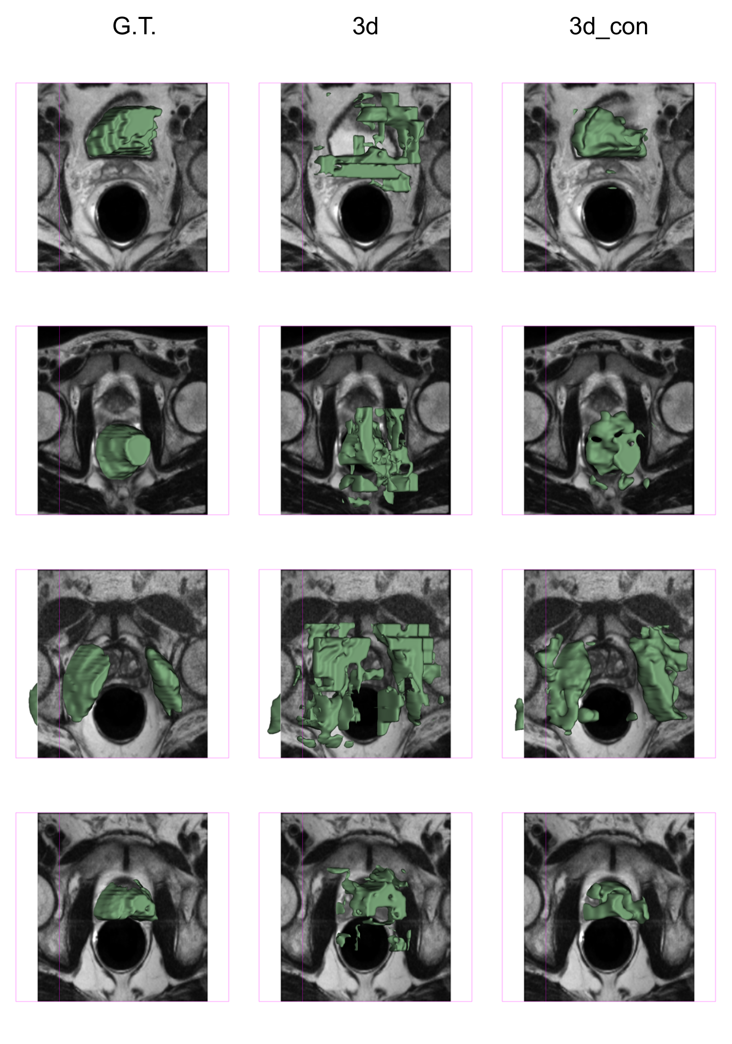
Adding support mask conditioning module alone (‘3d_con’) led , and absolute increase in Dice score comparing to ‘3d’, when support images came from all, base and novel institutions, respectively. Qualitatively, it predicted more “compact” segmentation with smoother boundary as shown in Fig. 9. However, it also resulted in a higher - a greater improvement was achieved when support and query came from the same institution, possibly because of its sensitivity to support-query (mis)alignment.
This was mitigated by the spatial registration mechanism which not only further improved the Dice score by but also reduced by . Fig. 10 shows an example where the target structure of the query and support were misaligned, resulting in segmentation failure. Aligning the support towards query, the spatial registration mechanism considerably improved the performance.
Interestingly, when spatial alignment mechanism was available, the support mask conditioning module led to a further improvement - , and absolute increase in Dice score from ‘3d_align’ to ‘3d_con_align’ when support images came from all, base and novel institutions, respectively.
It is also important to report that the proposed 3D network ‘3d’ without the support mask conditioning module and the spatial registration mechanism contained million parameters. It achieved comparable performance to the ‘2d’ baseline with million parameters, resulted in around reduction in number of parameters. For reference, the complete version of our proposed method ‘3d_con_align’ had contained 27.3 million parameters ( more parameters compared with ‘2d’), had achieved of relative Dice improvement over ‘2d’.
Furthermore, Table 6 and Table 7 report the mean Dice score achieved by ‘2d’ and ‘3d_con_align’ from different support-query institution combinations, when institution 3 is the novel institution. Better performance was often achieved by both methods when support images come from the query institution. A two tailed t-test is performed per query institution between the Dice scores where support institution equals query institution and the maximum Dice scores achieved when support institution differs from the query institution. Such observation is consistent with the hypothesis that the domain shift is smaller between support-query pairs within the same institution, leading to better performance.
Table 5 reports the performance of the proposed model (‘3d_con_align’) and baseline methods on novel classes, when both query and support come from base institutions while institution 3 is used as the novel institution. We report results when support come from the same institution as query, a different institution from query, and over all base institutions. The proposed method outperformed all baseline methods in few-shot setting, including two state-of-the-art methods - BiGRU [22] by 17.01%, 16.88% and 16.9% and LSNet [52] (which is adopted as our ‘2d’ baseline) by 9.39%, 13.37% and 12.88% absolute Dice, when support come from the same institution as query, different institution from query and all base institutions respectively, proving its efficacy even when no novel institution is involved during evaluation. Moreover, better performance was achieved when query and support came from the same institution than different institutions, with the performance gap reported as . The proposed method achieved smaller mean compare to baseline few-shot methods, suggesting its ability to mitigate domain shifts from cross-institution query and support data.
Table 8 reports the performance achieved by the proposed method (‘3d_con_align’) as training set varies. The performance dropped as the number of images inside the training set reduced. Notably, model trained on ‘half_single_ins’ performed worse than model trained on ‘quarter’, which had only half the size of ‘half_single_ins’. This suggests that the cross-institution few-shot task can be sensitive to the number of institutions available in the training set. To quantify this sensitivity is an interesting future research question.
Table 9 reports the performance of the proposed method ‘3d_con_align’ and ‘3d_finetune’ baseline, using 1 to 4 support examples (denoted as # shot). Performance improved for both methods, as the number of support examples increased. While ‘3d_finetune’ is more sensitive to the number of support examples, the proposed method still outperformed ‘3d_finetune’ using 1 to 4 support examples.
7 Discussion
While both the spatial registration mechanism and the support mask conditioning were motivated by the observation on multiple structure types found in the multi-institution data set used in this study, they may be promising to be beneficial for wider image types and anatomical regions as similar challenges were found in the few-shot segmentation of other types of non-medical data.
The labels used in this study were annotated by a mixture of clinicians and experienced medical imaging researchers. The estimated time for completing this task was more than one thousand observer-hours, a practically challenging task for most local hospitals if an alternative supervised learning was adopted for adopting or validating a segmentation tool. This further justifies the clinical relevance for the proposed few-shot segmentation approach.
It is noteworthy that the reported segmentation performance results were based on as few as 1 - 4 labelled training examples of the regions of interest, which had not been labelled in the model training stage.
Though challenging, cross-institutional few-shot segmentation could benefit situations when limited number of annotated data are available. Potential applications, although not investigated in this study due to relevant data availability, include specific pathology detection and segmentation with rare instances without previously observed occurrence in training institutions and longitudinal analysis with available within-subject data from individual patients.
Research questions remain for future research include the achievability or conditions to fill the gap to the upper-bound performance from supervised learning. For example, whether other types of data variance, such as scanner, imaging protocol and intensity in addition to the spatial domain studied in this work, need to be considered to improve cross-institution generalisability. Future work should aim to address these challenges for better performance, which we believe is very much plausible. These may yet be crucial in achieving clinically required accuracy for potential adoption in specific applications.
8 Conclusion
This paper described the first 3D prototypical learning algorithm for medical image segmentation, applied on multiple structures on pelvic MR images from different institutes. Substantial validation was based on clinical data from patients, with full segmentation of eight anatomical classes made available to the scientific community. The demonstrated novelty, efficacy, and clinical applicability of the proposed algorithm suggested an interesting direction for addressing the cost of expert labelling and cross-institute generalisation of current deep learning-based segmentation applications.
Acknowledgments
This work was supported by the International Alliance for Cancer Early Detection, a partnership between Cancer Research UK [C28070/A30912; C73666/A31378], Canary Center at Stanford University, the University of Cambridge, OHSU Knight Cancer Institute, University College London and the University of Manchester. This work was also supported by the Wellcome/EPSRC Centre for Interventional and Surgical Sciences [203145Z/16/Z], and EPSRC [EP/T029404/1, EP/S021930/1].
References
- Abdel-Basset et al. [2021] Abdel-Basset, M., Chang, V., Hawash, H., Chakrabortty, R.K., Ryan, M., 2021. Fss-2019-ncov: A deep learning architecture for semi-supervised few-shot segmentation of covid-19 infection. Knowledge-Based Systems 212, 106647.
- Bloch et al. [2015] Bloch, B.N., Jain, A., Jaffe, C.C., 2015. Data from prostate-diagnosis. The Cancer Imaging Archive doi:10.7937/K9/TCIA.2015.FOQEUJVT.
- Cardoso et al. [2022] Cardoso, M.J., Li, W., Brown, R., Ma, N., Kerfoot, E., Wang, Y., Murrey, B., Myronenko, A., Zhao, C., Yang, D., et al., 2022. Monai: An open-source framework for deep learning in healthcare. arXiv preprint arXiv:2211.02701 .
- Choyke et al. [2016] Choyke, P., Turkbey, B., Pinto, P., Merino, M., Wood, B., 2016. Data from prostate-mri. The Cancer Imaging Archive doi:10.7937/K9/TCIA.2016.6046GUDv.
- Cui et al. [2020] Cui, H., Wei, D., Ma, K., Gu, S., Zheng, Y., 2020. A unified framework for generalized low-shot medical image segmentation with scarce data. IEEE Transactions on Medical Imaging 40, 2656–2671.
- Dickinson et al. [2013] Dickinson, L., Ahmed, H.U., Kirkham, A., Allen, C., Freeman, A., Barber, J., Hindley, R.G., Leslie, T., Ogden, C., Persad, R., et al., 2013. A multi-centre prospective development study evaluating focal therapy using high intensity focused ultrasound for localised prostate cancer: the index study. Contemporary clinical trials 36, 68–80.
- Dong and Xing [2018] Dong, N., Xing, E.P., 2018. Few-shot semantic segmentation with prototype learning., in: BMVC.
- Feyjie et al. [2020] Feyjie, A.R., Azad, R., Pedersoli, M., Kauffman, C., Ayed, I.B., Dolz, J., 2020. Semi-supervised few-shot learning for medical image segmentation. arXiv preprint arXiv:2003.08462 .
- Fiorino et al. [1998] Fiorino, C., Reni, M., Bolognesi, A., Cattaneo, G.M., Calandrino, R., 1998. Intra-and inter-observer variability in contouring prostate and seminal vesicles: implications for conformal treatment planning. Radiotherapy and oncology 47, 285–292.
- Fu et al. [2019] Fu, Y., Robu, M.R., Koo, B., Schneider, C., Laarhoven, S.v., Stoyanov, D., Davidson, B., Clarkson, M.J., Hu, Y., 2019. More unlabelled data or label more data? a study on semi-supervised laparoscopic image segmentation, in: Domain Adaptation and Representation Transfer and Medical Image Learning with Less Labels and Imperfect Data. Springer, pp. 173–180.
- Gibson et al. [2018] Gibson, E., Hu, Y., Ghavami, N., et al., 2018. Inter-site variability in prostate segmentation accuracy using deep learning, in: International Conference on Medical Image Computing and Computer-Assisted Intervention, Springer. pp. 506–514.
- Guo et al. [2021] Guo, S., Xu, L., Feng, C., Xiong, H., Gao, Z., Zhang, H., 2021. Multi-level semantic adaptation for few-shot segmentation on cardiac image sequences. Medical Image Analysis 73, 102170.
- Hamid et al. [2019] Hamid, S., Donaldson, I.A., Hu, Y., et al., 2019. The smarttarget biopsy trial: a prospective, within-person randomised, blinded trial comparing the accuracy of visual-registration and magnetic resonance imaging/ultrasound image-fusion targeted biopsies for prostate cancer risk stratification. European urology 75, 733–740.
- Han and Fischl [2007] Han, X., Fischl, B., 2007. Atlas renormalization for improved brain mr image segmentation across scanner platforms. IEEE transactions on medical imaging 26, 479–486.
- He et al. [2020] He, Y., Li, T., Yang, G., Kong, Y., Chen, Y., Shu, H., Coatrieux, J.L., Dillenseger, J.L., Li, S., 2020. Deep complementary joint model for complex scene registration and few-shot segmentation on medical images, in: European Conference on Computer Vision, Springer. pp. 770–786.
- Henschel et al. [2020] Henschel, L., Conjeti, S., Estrada, S., Diers, K., Fischl, B., Reuter, M., 2020. Fastsurfer-a fast and accurate deep learning based neuroimaging pipeline. NeuroImage 219, 117012.
- Hosseini-Asl et al. [2016] Hosseini-Asl, E., Keynton, R., El-Baz, A., 2016. Alzheimer’s disease diagnostics by adaptation of 3d convolutional network, in: 2016 IEEE international conference on image processing (ICIP), IEEE. pp. 126–130.
- Howe and Matsuoka [1999] Howe, R.D., Matsuoka, Y., 1999. Robotics for surgery. Annual review of biomedical engineering 1, 211–240.
- Hu et al. [2018a] Hu, Y., Modat, M., Gibson, E., Ghavami, N., Bonmati, E., Moore, C.M., Emberton, M., Noble, J.A., Barratt, D.C., Vercauteren, T., 2018a. Label-driven weakly-supervised learning for multimodal deformable image registration, in: 2018 IEEE 15th International Symposium on Biomedical Imaging (ISBI 2018), IEEE. pp. 1070–1074.
- Hu et al. [2018b] Hu, Y., Modat, M., Gibson, E., Li, W., Ghavami, N., Bonmati, E., Wang, G., Bandula, S., Moore, C.M., Emberton, M., et al., 2018b. Weakly-supervised convolutional neural networks for multimodal image registration. Medical image analysis 49, 1–13.
- Hutchinson and Raff [2000] Hutchinson, M., Raff, U., 2000. Structural changes of the substantia nigra in parkinson’s disease as revealed by mr imaging. American journal of neuroradiology 21, 697–701.
- Kim et al. [2021] Kim, S., An, S., Chikontwe, P., Park, S.H., 2021. Bidirectional rnn-based few shot learning for 3d medical image segmentation, in: Proceedings of the AAAI Conference on Artificial Intelligence, pp. 1808–1816.
- Li et al. [2020] Li, A., Wang, S., Li, W., Liu, S., Zhang, S., 2020. Predicting human mobility with federated learning, in: Proceedings of the 28th International Conference on Advances in Geographic Information Systems, pp. 441–444.
- Li et al. [2021a] Li, X., Jiang, M., Zhang, X., Kamp, M., Dou, Q., 2021a. Fedbn: Federated learning on non-iid features via local batch normalization. arXiv preprint arXiv:2102.07623 .
- Li et al. [2021b] Li, Y., Data, G.W.P., Fu, Y., Hu, Y., Prisacariu, V.A., 2021b. Few-shot semantic segmentation with self-supervision from pseudo-classes. arXiv preprint arXiv:2110.11742 .
- Li et al. [2022] Li, Y., Fu, Y., Yang, Q., Min, Z., Yan, W., Huisman, H., Barratt, D., Prisacariu, V.A., Hu, Y., 2022. Few-shot image segmentation for cross-institution male pelvic organs using registration-assisted prototypical learning, in: 2022 IEEE 19th International Symposium on Biomedical Imaging (ISBI), IEEE. pp. 1–5.
- Litjens et al. [2015] Litjens, G., Futterer, J., Huisman, H., 2015. Data from prostate-3t. The Cancer Imaging Archive doi:10.7937/K9/TCIA.2015.QJTV5IL5.
- Litjens et al. [2014] Litjens, G., Toth, R., van de Ven, W., et al., 2014. Evaluation of prostate segmentation algorithms for mri: the promise12 challenge. Medical image analysis 18, 359–373.
- Liu et al. [2020] Liu, Y., Zhang, X., Zhang, S., He, X., 2020. Part-aware prototype network for few-shot semantic segmentation, in: European Conference on Computer Vision, Springer. pp. 142–158.
- Meyer et al. [2021] Meyer, A., Mehrtash, A., Rak, M., Bashkanov, O., Langbein, B., Ziaei, A., Kibel, A.S., Tempany, C.M., Hansen, C., Tokuda, J., 2021. Domain adaptation for segmentation of critical structures for prostate cancer therapy. Scientific reports 11, 1–14.
- Mondal et al. [2018] Mondal, A.K., Dolz, J., Desrosiers, C., 2018. Few-shot 3d multi-modal medical image segmentation using generative adversarial learning. arXiv preprint arXiv:1810.12241 .
- Ouyang et al. [2020] Ouyang, C., Biffi, C., Chen, C., et al., 2020. Self-supervision with superpixels: Training few-shot medical image segmentation without annotation, in: European Conference on Computer Vision, Springer. pp. 762–780.
- Perone et al. [2019] Perone, C.S., Ballester, P., Barros, R.C., Cohen-Adad, J., 2019. Unsupervised domain adaptation for medical imaging segmentation with self-ensembling. NeuroImage 194, 1–11.
- Petrella et al. [2003] Petrella, J.R., Coleman, R.E., Doraiswamy, P.M., 2003. Neuroimaging and early diagnosis of alzheimer disease: a look to the future. Radiology 226, 315–336.
- Ren et al. [2018] Ren, J., Hacihaliloglu, I., Singer, E.A., Foran, D.J., Qi, X., 2018. Adversarial domain adaptation for classification of prostate histopathology whole-slide images, in: International conference on medical image computing and computer-assisted intervention, Springer. pp. 201–209.
- Rieke et al. [2020] Rieke, N., Hancox, J., Li, W., Milletari, F., Roth, H.R., Albarqouni, S., Bakas, S., Galtier, M.N., Landman, B.A., Maier-Hein, K., et al., 2020. The future of digital health with federated learning. NPJ digital medicine 3, 1–7.
- De la Rosette et al. [2010] De la Rosette, J., Ahmed, H., Barentsz, J., Johansen, T.B., Brausi, M., Emberton, M., Frauscher, F., Greene, D., Harisinghani, M., Haustermans, K., et al., 2010. Focal therapy in prostate cancer—report from a consensus panel. Journal of Endourology 24, 775–780.
- Roy et al. [2020] Roy, A.G., Siddiqui, S., Pölsterl, S., et al., 2020. ‘squeeze & excite’guided few-shot segmentation of volumetric images. Medical image analysis 59, 101587.
- Shaban et al. [2017] Shaban, A., Bansal, S., Liu, Z., et al., 2017. One-shot learning for semantic segmentation. arXiv preprint arXiv:1709.03410 .
- Simmons et al. [2014] Simmons, L.A., Ahmed, H.U., Moore, C.M., Punwani, S., Freeman, A., Hu, Y., Barratt, D., Charman, S.C., Van der Meulen, J., Emberton, M., 2014. The picture study—prostate imaging (multi-parametric mri and prostate histoscanning™) compared to transperineal ultrasound guided biopsy for significant prostate cancer risk evaluation. Contemporary clinical trials 37, 69–83.
- Snell et al. [2017] Snell, J., Swersky, K., Zemel, R., 2017. Prototypical networks for few-shot learning. Advances in neural information processing systems 30.
- Sudre et al. [2017] Sudre, C.H., Li, W., Vercauteren, T., Ourselin, S., Jorge Cardoso, M., 2017. Generalised dice overlap as a deep learning loss function for highly unbalanced segmentations, in: Deep learning in medical image analysis and multimodal learning for clinical decision support. Springer, pp. 240–248.
- Sun et al. [2022] Sun, L., Li, C., Ding, X., Huang, Y., Chen, Z., Wang, G., Yu, Y., Paisley, J., 2022. Few-shot medical image segmentation using a global correlation network with discriminative embedding. Computers in biology and medicine 140, 105067.
- Sung et al. [2018] Sung, F., Yang, Y., Zhang, L., Xiang, T., Torr, P.H., Hospedales, T.M., 2018. Learning to compare: Relation network for few-shot learning, in: Proceedings of the IEEE conference on computer vision and pattern recognition, pp. 1199–1208.
- Tang et al. [2021] Tang, H., Liu, X., Sun, S., Yan, X., Xie, X., 2021. Recurrent mask refinement for few-shot medical image segmentation, in: Proceedings of the IEEE/CVF International Conference on Computer Vision, pp. 3918–3928.
- Tian et al. [2020] Tian, Z., Zhao, H., Shu, M., Yang, Z., Li, R., Jia, J., 2020. Prior guided feature enrichment network for few-shot segmentation. IEEE transactions on pattern analysis and machine intelligence .
- Tomar et al. [2021] Tomar, D., Lortkipanidze, M., Vray, G., Bozorgtabar, B., Thiran, J.P., 2021. Self-attentive spatial adaptive normalization for cross-modality domain adaptation. IEEE Transactions on Medical Imaging 40, 2926–2938.
- Wang et al. [2021] Wang, W., Xia, Q., Hu, Z., Yan, Z., Li, Z., Wu, Y., Huang, N., Gao, Y., Metaxas, D., Zhang, S., 2021. Few-shot learning by a cascaded framework with shape-constrained pseudo label assessment for whole heart segmentation. IEEE Transactions on Medical Imaging 40, 2629–2641.
- Weston et al. [2019] Weston, A.D., Korfiatis, P., Kline, T.L., Philbrick, K.A., Kostandy, P., Sakinis, T., Sugimoto, M., Takahashi, N., Erickson, B.J., 2019. Automated abdominal segmentation of ct scans for body composition analysis using deep learning. Radiology 290, 669–679.
- Xia et al. [2020] Xia, Y., Yang, D., Yu, Z., Liu, F., Cai, J., Yu, L., Zhu, Z., Xu, D., Yuille, A., Roth, H., 2020. Uncertainty-aware multi-view co-training for semi-supervised medical image segmentation and domain adaptation. Medical Image Analysis 65, 101766.
- Yan et al. [2022] Yan, W., Yang, Q., Syer, T., Min, Z., Punwani, S., Emberton, M., Barratt, D., Chiu, B., Hu, Y., 2022. The impact of using voxel-level segmentation metrics on evaluating multifocal prostate cancer localisation, in: Applications of Medical Artificial Intelligence: First International Workshop, AMAI 2022, Held in Conjunction with MICCAI 2022, Singapore, September 18, 2022, Proceedings, Springer. pp. 128–138.
- Yu et al. [2021] Yu, Q., Dang, K., Tajbakhsh, N., et al., 2021. A location-sensitive local prototype network for few-shot medical image segmentation, in: 2021 IEEE 18th International Symposium on Biomedical Imaging (ISBI), IEEE. pp. 262–266.
- Zhang et al. [2019] Zhang, C., Lin, G., Liu, F., Guo, J., Wu, Q., Yao, R., 2019. Pyramid graph networks with connection attentions for region-based one-shot semantic segmentation, in: Proceedings of the IEEE/CVF International Conference on Computer Vision.
- Zhao et al. [2019] Zhao, A., Balakrishnan, G., Durand, F., Guttag, J.V., Dalca, A.V., 2019. Data augmentation using learned transformations for one-shot medical image segmentation, in: Proceedings of the IEEE/CVF conference on computer vision and pattern recognition, pp. 8543–8553.
- Zhou et al. [2021] Zhou, H.Y., Liu, H., Cao, S., Wei, D., Lu, C., Yu, Y., Ma, K., Zheng, Y., 2021. Generalized organ segmentation by imitating one-shot reasoning using anatomical correlation, in: International Conference on Information Processing in Medical Imaging, Springer. pp. 452–464.