On the Optimization Landscape of Dynamic Output Feedback: A Case Study for Linear Quadratic Regulator
Abstract
The convergence of policy gradient algorithms in reinforcement learning hinges on the optimization landscape of the underlying optimal control problem. Theoretical insights into these algorithms can often be acquired from analyzing those of linear quadratic control. However, most of the existing literature only considers the optimization landscape for static full-state or output feedback policies (controllers). We investigate the more challenging case of dynamic output-feedback policies for linear quadratic regulation (abbreviated as dLQR), which is prevalent in practice but has a rather complicated optimization landscape. We first show how the dLQR cost varies with the coordinate transformation of the dynamic controller and then derive the optimal transformation for a given observable stabilizing controller. At the core of our results is the uniqueness of the stationary point of dLQR when it is observable, which is in a concise form of an observer-based controller with the optimal similarity transformation. These results shed light on designing efficient algorithms for general decision-making problems with partially observed information.
I Introduction
Reinforcement learning (RL) aims to directly learn optimal policies that minimize long-term cumulative costs through interacting with unknown environments. The past few years have witnessed great successes of RL in various domains, such as video games [1], robots control [2], nuclear fusion [3], and recommender systems [4]. Despite the impressive empirical performance of many policy gradient algorithms (such as DDPG [5], SAC [6], DSAC [7]), theoretical guarantees of their convergence, optimality, sample complexity, etc., remain unexplored and a big challenge.
As a case study, canonical optimal control of linear time-invariant (LTI) systems have been commonly analyzed to help reveal various theoretical properties of policy gradient methods [8, 9, 10, 11]. For example, recent investigations from the learning perspective show that the cost function of LQR enjoys an interesting property of gradient dominance [8, 10]. This enables a global linear convergence characterization for a variety of model-based and model-free gradient descent methods for solving LQR, such as policy gradient and actor-critic algorithms [8, 12], despite the non-convexity of optimizing the quadratic cost over the control gain. In addition, a series of subsequent studies examined the gradient dominance property for optimal control in different settings, including finite-horizon noisy LQR [13], LQR tracking [14], Markovian jump LQR [15], linear control with constraints [16], finite MDPs [17], and risk-constrained LQR [18].
The aforementioned literature mainly focuses on the case of static full state-feedback control. In many practical settings, the complete state information of the underlying system may not be directly available. Some recent works have studied static output-feedback (SOF) controllers to optimize a linear quadratic cost function [19, 20, 21, 22]. Different from the full state-feedback LQR, it is shown that policy gradient methods for solving optimal SOF controllers do not possess the gradient dominance property and thus are unlikely to find the globally optimal solution. In fact, the set of stabilizing SOF controllers is typically disconnected, and the stationary points can be local minima, saddle points, or even local maxima [20, 21]. Moreover, even finding a stabilizing SOF controller is a challenging task [23, 24].
This paper takes a step further to analyze the optimization landscape of the infinite-horizon dynamic output-feedback LQR (dLQR). From classical control theory, a stabilizing dynamic controller for dLQR can be found via designing separately a stable observer and a state-feedback controller thanks to the separation principle [25]. In the context of reinforcement learning, an observer-based dynamic controller can be learned through gradient descent optimization of the LQR cost. The very recent work [26] showed that gradient dominance condition does not hold for learning observer-based dynamic controller, and their analysis assumes complete knowledge of the system model. In contrast, we consider a model free setting, where we assume that a general full-order dynamic controller is learned directly from the LQR cost. The recent closely related work [27, 28] analyzed the structure of optimal dynamic controllers for the classical Linear Quadratic Gaussian (LQG) control problem. It was found that all stationary points that correspond to minimal controllers (i.e., whose state-space realization is reachable and observable) are globally optimal to LQG, and that these stationary points are identical up to coordinate (similarity) transformations. Different from LQG which considers stochastic linear systems and minimizes a limiting average cost (or the variance of the steady state), the dLQR seeks a dynamic controller that minimizes an infinite-horizon accumulated cost for a deterministic linear system. In the latter case, both the system transient dynamics induced by the initial system and controller states and the similarity transformation influence the cost, which suggests a more complicated optimization landscape. Notably, the existing analysis of LQG [27, 28, 26] does not extend to the dLQR directly. Indeed, little is known about the optimality of the converged solutions of policy gradient methods for dLQR.
In this paper, we provide a comprehensive analysis of the influence of similarity transformation and the structure of the stationary points. Specifically,
- 1.
We analyze the impact of similarity transformations on the dLQR cost and derive an explicit form of the unique optimal similarity transformation for a given observable stabilizing controller.
- 2.
We characterize the unique observable stationary point of the dLQR cost, which is in a concise form of an observer-based controller with the optimal similarity transformation.
The remainder of this paper is organized as follows. Section II presents the problem statement of the dLQR problem, and Section III derives an analytical form of the dLQR cost as a function of dynamic controller parameters. Section IV analyzes the impact of similarity transformations on the dLQR cost. Section V characterizes the structure of the observable stationary controller. The paper is concluded in Section VI.
Notation: We use to denote the set of natural numbers. Given a matrix , , , , and denote its spectral radius, trace, minimum eigenvalue, and Frobenius norm, respectively. (respectively, ) denotes the set of symmetric positive semidefinite (respectively, positive definite) matrices. Finally, denotes the set of invertible matrices, and denotes the identity matrix.
II Problem Statement
In this section, we start with the canonical linear quadratic optimal control problem, and then present the dynamic output-feedback Linear Quadratic Regulator (dLQR).
II-A Linear Quadratic Control
Consider a discrete-time linear time-invariant (LTI) system
| (1) | ||||
where , , are system matrices, and , , are the system state, input, and output measurements at time , respectively. The linear quadratic control seeks a sequence minimizing the infinite-horizon accumulated cost:
| (2) | ||||
where and are performance weights, the initial state is randomly distributed according to a given distribution , and the control input at time is allowed to depend on the historical outputs and inputs . The initial state distribution has been commonly introduced to model the randomness of initial states [8, 29, 11] in a data-driven learning setting. For problem (2), the following assumption is standard:
Assumption 1.
is controllable, and and are observable.
Without loss of generality, we assume has full row rank. The state-feedback LQR corresponds to . In this special case, the globally optimal controller is a static linear feedback , where can be obtained via solving a Riccati equation [30]. In general cases where , a static output-feedback (SOF) gain with is typically insufficient to obtain good control performance. In fact, the set of stabilizing SOF gains can be highly disconnected [21], and even finding a stabilizing SOF controller is generally a challenging task [23, 24]. Unlike SOF control, under Assumption 1, a stabilizing dynamic output controller always exists and can be found easily, thanks to the well-known separation principle [25].
II-B The dLQR Problem
More generally, we consider the class of full-order dynamic output-feedback controllers in the form of11 1 This is in the standard form of strictly proper dynamic controllers, where there is no direct feed-through of to [27, 28, 31].
| (4) | ||||
where is the internal state of the controller, and matrices , , are the controller parameters to be learned. The observer-based controller (3) is a special case of (4). Note that the controller parameterization in (4) does not explicitly rely on the knowledge of system parameters , , and , which allows for model-free policy learning.
In addition to , , and , the transient behavior induced by the initial controller state (or initial state estimate) also affects the accumulated cost. Let be the initial state estimate and suppose follows a joint distribution . The dynamic output-feedback LQR (dLQR) which aims to minimize the accumulated linear quadratic cost [32, 33, 34, 35] is given by
| (5) | ||||
III Optimization formulation of the dLQR Problem
In this section, we derive the analytical form of the cost function (5) in terms of the dynamic controller parameters, which is needed for analyzing its optimization landscape.
We start by combining (4) with (1) and get the closed-loop system
| (6) |
We further denote
and write the controller parameters in a compact form
Then (6) can be expressed as
| (7) |
The set of all stabilizing controllers is given by
| (8) |
It is known that is non-convex but has at most two disconnected components [27, 28]. Upon denoting
the dLQR problem (5) can be written as
| (9) | ||||
For the LTI system (7), the value function of state under a stabilizing controller takes a quadratic form as
where . Define the state correlation matrix under a stabilizing controller as
For each , with and , it is well known that the dLQR cost value in (9) can be computed in the following lemma [27, 8].
Lemma 1.
Given each , the dLQR cost value is
| (10) |
where and are the unique positive semidefinite solutions to the following Lyapunov equations
| (11a) | ||||
| (11b) | ||||
with .
Note that can be partitioned into four matrices:
| (12) |
Similarly, one has
| (13) |
Finally, we formulate the dLQR problem (5) into the following optimization form.
Note that the initial estimate is sampled from a fixed initial distribution, and thus the matrix in (11b) is independent of the parameters .
Next, we will characterize several important properties that delineate the optimization landscape (such as the influence of similarity transformation and structure of stationary points) of policy gradient methods for solving Problem 1. The detailed proofs are provided in the Appendix.
IV dLQR Cost under Different Similarity Transformations
For dynamic controllers, a widely used concept is the so-called similarity transformation [36]. It is well-known that similarity transformations do not change the control performance of the LQG problem [28, Lemma 4.1]. However, in this section, we will show that the dLQR cost varies with different similarity transformations due to the transient behavior induced by initial controller states, and thus the optimization landscape of dLQR is distinct from LQG.
IV-A Varying dLQR cost
Given a controller and an invertible matrix , we define the similarity transformation on by
| (14) |
It is not hard to verify that if and , we have ; see [28, Lemma 3.2] for further discussions.
Our first result reveals that the dLQR cost is not invariant w.r.t. the similarity transformation (14). Indeed, we have the following result.
Proposition 1.
Although any similarity transformation corresponds to the same transfer function in the frequency domain, Proposition 1 shows that the dLQR cost varies with different similarity transformations. This result is reasonable considering the facts that the initial controller state is assumed to follow a fixed distribution and that the similarity transformation implies a coordinate change of the internal controller state. If the controller coordinate changes while its initial state does not change, this essentially leads to a different dynamic controller (4), which naturally results in a different dLQR cost value.
IV-B Optimal similarity transformation
One natural consequence of Proposition 1 is that for each stabilizing controller , there might exist an optimal similarity transformation matrix in the sense that
| (16) |
In this case, we call the optimal similarity transformation matrix of .
In this paper, we refer to (4) as an observable controller if is observable. We denote the set of observable controllers as
Our next result characterizes the structure of the optimal similarity transformation for an observable stabilizing controller.
Theorem 1.
Theorem 1 identifies the form of the optimal similarity transformation, which is unique if it exists. This implies that if the optimal controller for Problem 1 is observable, it may be unique and be expressed as an optimal similarity transformation of a particular dynamic controller. However, the optimal similarity transformation may not always exist since can be singular. We give such an analytical example in Section -B.
We conclude this section by providing two examples to illustrate the impact of similarity transformation on the dLQR cost.
Example 1.
Consider an open-loop unstable dynamic system (1) with
According to [28, Theoerem D.4, Example 11], the set of stabilizing controllers for this system has two disconnected components. To define dLQR (5), we choose
| (18) |
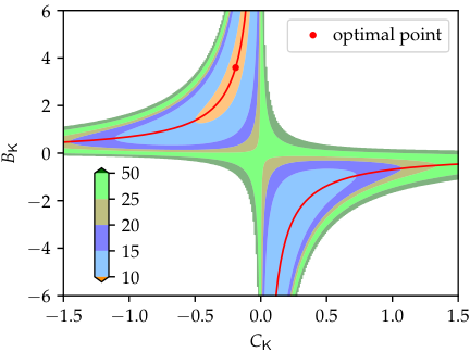
For each observable stabilizing controller , Theorem 1 implies that there exists an optimal transformation that leads to the lowest dLQR cost. Fig. 1a demonstrates this fact. In particular, the red line of Fig. 1a displays the orbit of the similarity transformation of controller
We can see that the dLQR cost changes with different similarity transformations, which also shows that finding the optimal similarity transformation (marked as the red point) can significantly improve the control performance.
Example 2.
Consider an open-loop stable dynamic system (1) with
According to [28, Theoerem D.4], the set of stabilizing controllers for this system is nonconvex but connected. To define dLQR (5), we choose as (18). Again, for each observable stabilizing controller , Theorem 1 implies that there exists an optimal transformation, shown in Fig. 1b, where the red line displays the orbit of the similarity transformation of controller
and the red point represents the optimal similarity transformation.

V Structure of Stationary Points
In this section, we characterize the stationary points of Problem 1 by letting the gradients of the dLQR cost be zero. Upon denoting the gradient of w.r.t. , , and as , , and , respectively, we define the set of stationary points as
We now look into the structure of , which is crucial for understanding the performance of policy gradient methods on dLQR problems.
Theorem 2.
Suppose has full row rank, , and Assumption 1 holds. If an observable stationary point, i.e., , to Problem 1 exists, it is unique and in the form of
| (19) |
where
| (20) |
is the optimal transformation matrix of given in (17) with , and
| (21) |
| (22) |
with and being the unique positive definite solutions to
| (23) |
| (24) |
In Theorem 2, is an elegant closed-form solution since it satisfies the optimal similarity transformation of a special observer-based controller . Note that of (20) is exactly the optimal control gain of the state-feedback LQR and is a stable observer gain. In classical control theory [25], the observer-based controller of Problem 1 can separate into a stable observer and a state-feedback LQR; however, the transient behavior induced by the initial state and estimate is not considered. As a comparison, both the observer gain and the optimal transformation matrix of the observable stationary point are uniquely determined according to the prior information of the initial distribution of system state and controller state .
Note that Theorem 2 does not discuss the theoretical optimality of the identified stationary point, which will be of interest for future work. In practical applications, if the optimal controller of a given system is known to be observable, then in (19) must be the globally optimal controller due to its uniqueness. For instance, the observable stationary points of Examples 1 and 2, i.e.,
are globally optimal by Theorem 2. They agree with the exhausted numerical grid search for the globally optimal points (marked as red points in Fig. 1) in Examples 1 and 2, respectively.
VI Conclusion
In this paper, we have analyzed the policy gradient optimization landscape of linear quadratic control problems using dynamic output-feedback policies. We have shown that the dLQR cost varies with similarity transformations, and identified the structure of the optimal similarity transformation of an observable stabilizing controller. More importantly, we characterized the stationary point of the policy gradient optimization and proved that the associated dynamic controller is unique if it is observable. Our work brings new insights for understanding the policy gradient algorithms for solving the partially observed control or decision-making problems.
-A Block-wise Lyapunov equations and useful lemmas
The block-wise Lyapunov equations in (11a) and (11b) will be used extensively in this paper. From (11a), we have
| (25a) | ||||
| (25b) | ||||
| (25c) | ||||
Similarly, we get
| (26a) | ||||
| (26b) | ||||
| (26c) | ||||
Standard Lyapunov theorems will be used throughout the paper. We summarize them below for completeness.
Lemma 2 (Lyapunov stability theorems [37, 29]).
- (a)
If and , the Lyapunov equation has a unique solution .
- (b)
Let . if and only if there exists a unique such that .
- (c)
Suppose is observable. if and only if there exists a unique such that .
Given an observable stabilizing controller, the following lemma is a discrete-time counterpart to [28, Lemma 4.5].
-B Non-existence of the optimal similarity transformation
We take a one-dimensional system as an example (i.e., and are scalars), to show the non-existence of the optimal similarity transformation if is singular. Under similarity transformation (14), we have
| (27) | ||||
Given an observable stabilizing controller , by (17) of Theorem 1, one has
| (28) |
Note that the cross-correlation value if the initial controller state is zero-mean and independent of the initial system state . Using (28) in (27), we can observe that the controller input tends to ignore the influence of by increasing in this one-dimensional instance. This is because that the initial controller state provides no information for the estimation of the initial system state if .
-C Proof of Proposition 1
-D Proof of Theorem 1
Proof.
By (15), can be expressed as
| (31) | ||||
For notational convenience, given a stabilizing controller , we denote the cost value w.r.t. similarity transformation as
It is clear that is twice differentiable w.r.t. . The gradient of w.r.t. can be derived as
| (32) |
By Lemma 3, the solution to (11a) is positive definite, which means is invertible. We also have that is invertible since . Let , we have
By , we now identify is in the form of (17). This also implies that if exists, both and must be invertible.
Next, we show that in (17) is the unique globally optimal similarity transformation matrix such that (16) holds. We analyze the Hessian of applied to a nonzero direction , which is
By (31), we can further show that
We extend the function to be defined on a convex superset of . It is immediate that is strongly convex over , which means the globally optimum of over is unique when it exists. By , then the globally optimum of is also unique over , thus (16) is satisfied for a unique . ∎
-E Policy Gradient Expression
Lemma 4 (Policy Gradient Expression).
For , the policy gradient of Problem 1 is
| (33a) | ||||
| (33b) | ||||
| (33c) | ||||
Proof.
The proof follows the similar lines as the state-feedback LQR case [8, Lemma 1]. By (11a), the value function of reads as
Taking the gradient of w.r.t. (note that has two terms: one with respect to in the subscript and one with respect to the input ), we have
where the last step uses recursion and that .
We can also derive the formulas of and through similar steps. Then, we can finally observe (33) by taking the expectation w.r.t. the initial distribution . ∎
-F Proof of Theorem 2
Proof.
Suppose an observable stationary point exists, denoted as . By Lemma 2(b) and Lemma 3, we know . By the Schur complement, it is obvious that
Throughout this proof, the subscript of the submatrices of and under observable stationary point will be omitted. Since (33) is linear in , , and , when , it is not hard to show that
| (34a) | ||||
| (34b) | ||||
| (34c) | ||||
where and are
Combining (25b), (25c), and (34), we prove that
| (35) |
which immediately leads to
| (36) |
We then define , and thus . Similarly, from (26b), (26c), and (34), (35) can be rewritten as
| (37) |
Combining (35) with (37) leads to
| (38) |
Combining (34), (36), and (38), we can observe that is in the form shown in (19).
It remains to show that
- •
is the optimal transformation matrix of given in (17) (i.e., );
- •
First, by (19) and (30) in Proposition 1, we have
From (37), it is not hard to show that
which directly leads to Therefore, by (17) of Theorem 1, one has
which is exactly the optimal transformation matrix of .
Then, we will derive (24). Multiplying (25c) by on the left and by on the right (or multiplying (25b) by on the right), we have
| (39) | ||||
Then, plugging (34b) in (25a) leads to
| (40) | ||||
Subtracting (39) from (40), we can finally see that satisfies the Riccati equation (24). Through similar steps, we can derive from (26) that satisfies the Riccati equation (23), which completes the proof. ∎
References
- [1] V. Mnih, K. Kavukcuoglu, D. Silver, A. A. Rusu, J. Veness, M. G. Bellemare, A. Graves, M. Riedmiller, A. K. Fidjeland, G. Ostrovski, et al., “Human-level control through deep reinforcement learning,” Nature, vol. 518, no. 7540, pp. 529–533, 2015.
- [2] H. Nguyen and H. La, “Review of deep reinforcement learning for robot manipulation,” in 2019 Third IEEE International Conference on Robotic Computing (IRC), pp. 590–595, IEEE, 2019.
- [3] J. Degrave, F. Felici, J. Buchli, M. Neunert, B. Tracey, F. Carpanese, T. Ewalds, R. Hafner, A. Abdolmaleki, D. de Las Casas, et al., “Magnetic control of tokamak plasmas through deep reinforcement learning,” Nature, vol. 602, no. 7897, pp. 414–419, 2022.
- [4] L. Zou, L. Xia, Z. Ding, J. Song, W. Liu, and D. Yin, “Reinforcement learning to optimize long-term user engagement in recommender systems,” in Proceedings of the 25th ACM SIGKDD International Conference on Knowledge Discovery & Data Mining, pp. 2810–2818, 2019.
- [5] T. P. Lillicrap, J. J. Hunt, A. Pritzel, N. Heess, T. Erez, Y. Tassa, D. Silver, and D. Wierstra, “Continuous control with deep reinforcement learning,” in 4th International Conference on Learning Representations (ICLR 2016), (San Juan, Puerto Rico), 2016.
- [6] T. Haarnoja, A. Zhou, P. Abbeel, and S. Levine, “Soft actor-critic: Off-policy maximum entropy deep reinforcement learning with a stochastic actor,” in Proceedings of the 35th International Conference on Machine Learning (ICML 2018), (Stockholmsmässan, Stockholm Sweden), pp. 1861–1870, PMLR, 2018.
- [7] J. Duan, Y. Guan, S. E. Li, Y. Ren, Q. Sun, and B. Cheng, “Distributional soft actor-critic: Off-policy reinforcement learning for addressing value estimation errors,” IEEE Transactions on Neural Networks and Learning Systems, 2021.
- [8] M. Fazel, R. Ge, S. Kakade, and M. Mesbahi, “Global convergence of policy gradient methods for the linear quadratic regulator,” in International Conference on Machine Learning, pp. 1467–1476, PMLR, 2018.
- [9] J. Bu, A. Mesbahi, M. Fazel, and M. Mesbahi, “LQR through the lens of first order methods: Discrete-time case,” arXiv preprint arXiv:1907.08921, 2019.
- [10] H. Mohammadi, A. Zare, M. Soltanolkotabi, and M. R. Jovanović, “Global exponential convergence of gradient methods over the nonconvex landscape of the linear quadratic regulator,” in 2019 IEEE 58th Conference on Decision and Control (CDC), pp. 7474–7479, IEEE, 2019.
- [11] D. Malik, A. Pananjady, K. Bhatia, K. Khamaru, P. Bartlett, and M. Wainwright, “Derivative-free methods for policy optimization: Guarantees for linear quadratic systems,” in The 22nd International Conference on Artificial Intelligence and Statistics, pp. 2916–2925, PMLR, 2019.
- [12] Z. Yang, Y. Chen, M. Hong, and Z. Wang, “Provably global convergence of actor-critic: A case for linear quadratic regulator with ergodic cost,” Advances in neural information processing systems, vol. 32, 2019.
- [13] B. M. Hambly, R. Xu, and H. Yang, “Policy gradient methods for the noisy linear quadratic regulator over a finite horizon,” Available at SSRN, 2020.
- [14] Z. Ren, A. Zhong, and N. Li, “LQR with tracking: A zeroth-order approach and its global convergence,” in 2021 American Control Conference (ACC), pp. 2562–2568, IEEE, 2021.
- [15] J. P. Jansch-Porto, B. Hu, and G. Dullerud, “Policy optimization for markovian jump linear quadratic control: Gradient-based methods and global convergence,” arXiv preprint arXiv:2011.11852, 2020.
- [16] K. Zhang, B. Hu, and T. Basar, “Policy optimization for linear control with robustness guarantee: Implicit regularization and global convergence,” in Learning for Dynamics and Control, pp. 179–190, PMLR, 2020.
- [17] J. Bhandari and D. Russo, “Global optimality guarantees for policy gradient methods,” arXiv preprint arXiv:1906.01786, 2019.
- [18] F. Zhao and K. You, “Primal-dual learning for the model-free risk-constrained linear quadratic regulator,” in Learning for Dynamics and Control, pp. 702–714, PMLR, 2021.
- [19] J. Duan, J. Li, S. E. Li, and L. Zhao, “Optimization landscape of gradient descent for discrete-time static output feedback,” in 2022 American Control Conference (ACC), (Atlanta, Georgia, USA), pp. 2932–2937, IEEE, 2022.
- [20] I. Fatkhullin and B. Polyak, “Optimizing static linear feedback: Gradient method,” SIAM Journal on Control and Optimization, vol. 59, no. 5, pp. 3887–3911, 2021.
- [21] H. Feng and J. Lavaei, “Connectivity properties of the set of stabilizing static decentralized controllers,” SIAM Journal on Control and Optimization, vol. 58, no. 5, pp. 2790–2820, 2020.
- [22] J. Bu, A. Mesbahi, and M. Mesbahi, “On topological and metrical properties of stabilizing feedback gains: the mimo case,” arXiv preprint arXiv:1904.02737, 2019.
- [23] V. Blondel and J. N. Tsitsiklis, “Np-hardness of some linear control design problems,” SIAM Journal on Control and Optimization, vol. 35, no. 6, pp. 2118–2127, 1997.
- [24] V. L. Syrmos, C. T. Abdallah, P. Dorato, and K. Grigoriadis, “Static output feedback—a survey,” Automatica, vol. 33, no. 2, pp. 125–137, 1997.
- [25] F. L. Lewis, D. Vrabie, and V. L. Syrmos, Optimal control. John Wiley & Sons, 2012.
- [26] H. Mohammadi, M. Soltanolkotabi, and M. R. Jovanovic, “On the lack of gradient domination for linear quadratic gaussian problems with incomplete state information,” pp. 2562–2568, 2021.
- [27] Y. Tang, Y. Zheng, and N. Li, “Analysis of the optimization landscape of linear quadratic gaussian (LQG) control,” in Learning for Dynamics and Control, pp. 599–610, PMLR, 2021.
- [28] Y. Zheng, Y. Tang, and N. Li, “Analysis of the optimization landscape of linear quadratic gaussian (LQG) control,” arXiv preprint arXiv:2102.04393, 2021.
- [29] D. Lee and J. Hu, “Primal-dual Q-learning framework for LQR design,” IEEE Transactions on Automatic Control, vol. 64, no. 9, pp. 3756–3763, 2018.
- [30] D. Bertsekas, Dynamic programming and optimal control: Volume I, 4th Edition. Athena scientific, 2017.
- [31] H. J. Van Waarde, J. Eising, H. L. Trentelman, and M. K. Camlibel, “Data informativity: a new perspective on data-driven analysis and control,” IEEE Transactions on Automatic Control, vol. 65, no. 11, pp. 4753–4768, 2020.
- [32] H. Modares, F. L. Lewis, and Z.-P. Jiang, “Optimal output-feedback control of unknown continuous-time linear systems using off-policy reinforcement learning,” IEEE Transactions on Cybernetics, vol. 46, no. 11, pp. 2401–2410, 2016.
- [33] S. A. A. Rizvi and Z. Lin, “Output feedback q-learning for discrete-time linear zero-sum games with application to the h-infinity control,” Automatica, vol. 95, pp. 213–221, 2018.
- [34] S. A. A. Rizvi and Z. Lin, “Reinforcement learning-based linear quadratic regulation of continuous-time systems using dynamic output feedback,” IEEE transactions on cybernetics, vol. 50, no. 11, pp. 4670–4679, 2019.
- [35] S. A. A. Rizvi and Z. Lin, “Output feedback adaptive dynamic programming for linear differential zero-sum games,” Automatica, vol. 122, p. 109272, 2020.
- [36] K. Zhou, J. C. Doyle, and K. Glover, “Robust and optimal control,” 1996.
- [37] G. Gu, Discrete-time linear systems: theory and design with applications. Springer Science & Business Media, 2012.