Multi-modal Streaming 3D Object Detection
Abstract
Modern autonomous vehicles rely heavily on mechanical LiDARs for perception. Current perception methods generally require point clouds, collected sequentially as the LiDAR scans the azimuth and acquires consecutive wedge-shaped slices. The acquisition latency of a full scan () may lead to outdated perception which is detrimental to safe operation. Recent streaming perception works proposed directly processing LiDAR slices and compensating for the narrow field of view (FOV) of a slice by reusing features from preceding slices. These works, however, are all based on a single modality and require past information which may be outdated. Meanwhile, images from high-frequency cameras can support streaming models as they provide a larger FoV compared to a LiDAR slice. However, this difference in FoV complicates sensor fusion. To address this research gap, we propose an innovative camera-LiDAR streaming 3D object detection framework that uses camera images instead of past LiDAR slices to provide an up-to-date, dense, and wide context for streaming perception. The proposed method outperforms prior streaming models on the challenging NuScenes benchmark. It also outperforms powerful full-scan detectors while being much faster. Our method is shown to be robust to missing camera images, narrow LiDAR slices, and small camera-LiDAR miscalibration.
Index Terms:
RGB-D Perception, sensor fusion, streaming 3D object detection.I INTRODUCTION
Safe navigation for autonomous vehicles (AVs) requires minimal latency in perception, especially in dynamic environments. Dominant LiDAR-based 3D object detectors often rely on rotational LiDARs to provide a point cloud of the scene around an AV [1, 2, 3]. A full LiDAR sweep is composed of a stream of slices/packets collected sequentially as the LiDAR scans the azimuth. These detectors must wait for a full LiDAR scan () before inference which presents a bottleneck for perception latency. This delay can lead to outdated detections which is detrimental to safe autonomous driving [4, 5], as shown in Fig. 1.

Instead of waiting for a full scan, [4] proposed directly taking a slice (once it arrives) as input for detection models. While processing LiDAR slices reduces latency, the narrow field of view (FoV) of a slice results in less available context for the model to learn and infer from, thus resulting in lower accuracy. This is especially problematic for objects close to the ego-vehicle (the most safety-critical). A slice may only contain a fragment of an object, as shown in Fig. 1. To tackle this problem, all prior work on streaming 3D detection [4, 5, 6] have utilized memory mechanisms and features from past slices to provide a global context.
The use of past features is not ideal (especially in dynamic scenes) since it expands the current context with outdated information. A vehicle with a speed of 60 km/h moves nearly 1.7 m during a single scan by a 10 Hz LiDAR. An object of interest in previous slices may no longer be in the same position when processing the current slice due to the fast movement of objects, sudden occlusion, or a multitude of different factors inherent in a dynamic environment. These are issues that simple ego-motion compensation cannot fix, since it does not address the motion of other objects and it can be error prone [7]. Errors resulting from using past LiDAR features will aggregate and affect downstream tasks.
This concern has not been addressed previously in streaming perception [4, 5, 6]. One reason could be that the artificial experimental setup of prior studies relied on relatively static LiDAR scans (discussed in Sec. II). Also, the use of features from past slices relies on two assumptions that may not hold in practice: 1) that slice inference time is shorter than the arrival rate of slices, and 2) that past slices truly represent the current world. If 1) fails, then a sequential bottleneck arises where arriving slices wait for prior slices to be processed. If 2) fails, then we get outdated or misinformed perception.

.
Meanwhile, cameras are widely deployed on AVs and usually acquire images at a high rate. Images also provide a wider FoV than a LiDAR slice, which makes them ideal in providing a global context for streaming detection. Dominant camera-LiDAR fusion methods [8, 9, 10, 3, 11] rely on point-wise operations and require a matching FoV between LiDAR and camera data. In our streaming setting however, the FoV overlap between a camera and a narrow LiDAR slice is small. Thus, existing fusion methods are not suited for our problem.
To bridge the above research gap, we propose a multi-modal streaming 3D object detection framework that utilizes camera images to provide a current global context to a LiDAR slice using an innovative fusion method. The difference in FoV between the two modalities is addressed by extracting the features of each modality (an image and a LiDAR slice) independently and in parallel. These features are then projected to a unified spatial Birds Eye View (BEV) representation. This representation is processed by convolutional neural networks (CNNs) and sent to a detection head for 3D bounding box prediction. We also propose a feature map cropping operation that significantly speeds up the forward pass while maintaining cross-modal spatial relations. Our contributions are as follows:
- 1.
We propose the first framework for multi-modal streaming detection that effectively uses camera images to complement narrow LiDAR slices.
- 2.
This framework outperforms prior streaming methods without relying on past LiDAR slices. It also outperforms representative single and multi-modal full-scan detectors while taking only a LiDAR slice as input.
- 3.
Our method encodes each modality separately and does not depend on past slices. This parallelism can be exploited by GPUs or FPGAs to further reduce latency.
- 4.
Experiments show the benefits of the proposed method and its robustness to small camera-LiDAR miscalibration, missing camera images, and very narrow LiDAR slices (see Fig. 1). We also discuss the runtime and computational cost of the proposed framework.
II RELATED WORK
LiDAR-Based 3D Detection
Processing a LiDAR point cloud for 3D object detection usually involves one of the following three representations: The 1st is voxelizing the input into 3D grids and extracting features using 3D CNNs or sparse convolutions [12, 13]. While accurate, these models are computationally expensive and depend on voxel resolution. The 2nd is processing the point cloud as a dense range image [14, 15]. This representation, while efficient, suffers from object overlap, and sizes varying with depth. The third and most popular is the top-down BEV which maintains constant object sizes, although it is much sparser than range images [2, 16]. This representation has shown great performance for 3D detection since it simplifies the localization task and utilizes 2D CNNs for efficiency.
LiDAR-Camera Fusion
Early fusion work relied on point-wise sampling of image features across multiple scales [8, 9]. However, these methods are complicated and often suffer from feature blurring. Recently, simpler and more effective methods proposed decorating each 3D point with image features [3] or segmentation scores [10]. Most prior work on fusion combines information from both modalities in a point-wise fashion and requires matching FoVs between the two modalities. Point-wise methods are thus not suited for our streaming problem where the camera images provide a wider FoV than the narrow LiDAR slices.
Moreover, point-wise fusion methods require extremely accurate camera-LiDAR calibration which can degrade with operation [17]. Yoo et al. [18] use auto-calibration to project image features to BEV and attention mechanisms to fuse multi-modal features during encoding and at the region refinement stage. Our method differs from prior work in that it is fully convolutional, designed specifically for streaming detection, avoids strict point-wise fusion, and significantly improves the LiDAR-only baseline.
Streaming 3D Object Detection
Streaming detection is a relatively new direction with limited prior work. Nonetheless, it was shown to be effective in replacing full sweeps for more latency-efficient perception. Han et al. [4] proposed modifying the meta-architecture of full-scan 3D detectors to facilitate operating on streaming LiDAR slices. They used recurrent neural networks to preserve features from past slices and pass them to the current slice, thus expanding the context and restoring the degraded accuracy due to streaming. Frossard et al. [5] proposed storing multi-scale feature maps from past slices and concatenating them with current slice features. Finally, Chen et al. [6] pointed that slices are better represented in polar coordinates. They used BEV “polar pillars” and padded past slice features to current features along the azimuth dimension.
Such past-aware solutions were able to compensate for most of the context lost due to the narrow streaming input. However, we argue that such good results are mainly a consequence of an unrealistic experimental setup. All prior streaming detection works simulate a streaming input by slicing a relatively static LiDAR scan (collected by slow vehicles) into slices. This makes the same false assumption (that LiDAR points are observed synchronously) as full-scan models; and therefore past features from many prior slices are sufficient to replenish the model. However in reality, a streaming input is dynamic and past features would represent an outdated state of the world as discussed in Sec. I. This is a main motivation behind our work: we replace past LiDAR slices with up-to-date images.
III Multi-modal Streaming 3D Detection
An overview of the proposed framework is shown in Fig. 2. It takes as input a LiDAR point cloud slice and camera images encompassing the slice and outputs detected objects within a slice. Each modality goes through a separate encoding pipeline for feature extraction (Sec. III-A). We present a novel method to project dense 2D image features to BEV using an intermediate 3D volumetric representation. The resulting multi-modal BEV representations are then fused, encoded, and sent through a detection head (Sec. III-B). Finally, to speed up inference, a feature map cropping method is proposed in Sec. III-C.
III-A Multi-modal Feature Extraction
Features from both input modalities are extracted independently and in parallel. The goal is to have these features in a common spatial (BEV) and feature space for fusion.
III-A1 Point Cloud Encoding
First, the 3D point cloud slice is transformed into a BEV feature map. A PointPillars [16] encoder is adopted as it well-balances accuracy and speed. Each point is represented with a vector where denote the 3D location, and denote reflectance and relative timestamp. We add the slice index to allow the model to learn slice-specific information. The scene is divided into a top-down BEV grid. Points within each pillar (grid pixel) are encoded using a PointNet [19]. This gives each pillar a feature vector of size . Overall, this stream produces a 2D BEV feature map .
III-A2 Camera Image Encoding
Let be the -th input image from images. A pre-trained ResNet-50 [20] backbone is used to extract multi-scale 2D feature maps from each image. Afterwards a feature pyramid network (FPN) [21] is used to aggregate these feature maps into . This stream produces semantically-rich 2D feature maps from images around a LiDAR slice.
III-A3 Discussion
Feature extraction for each modality is separate. This allows the fusion process to be independent of point-wise or sequential operations. This is motivated by three reasons: First, independent encoding allows for retaining the complementary information from both modalities. For example, image features are not simply appended to sparse and narrow point cloud slices [10] and thus losing their richness and density. This allows image features to provide needed context that is wider than the slice. Second, independent encoding boosts robustness to small camera-LiDAR miscalibration, missing points, or missing camera images as discussed in Sec. IV. Third, parallel encoding allows for better utilization of parallelization hardware.

III-B Multi-modal Fusion
III-B1 Projection and 3D Convolutions
To widen the 3D context around a LiDAR slice, 2D image features must be projected to a common spatial and feature space with the point cloud features. Given image feature maps , projection is done as follows: The scene is divided into a 3D grid . This is the same voxel size used to grid the point cloud input in the plane. However, instead of pillars there are multiple -high voxels along the z-axis. Projection is done using perspective mapping from the pinhole camera model, and the intrinsic and extrinsic matrices of each camera. To project an pixel to 3D voxels we use Eqn. 1. All voxels along a ray that passes through a pixel will be filled with its features. Voxels outside the FoV of a camera are padded with zeros. If multiple pixels project to the same 3D voxel (intersecting camera FoVs), their features are averaged. Now image features are in 3D space .
| (1) |
The projected image features are then transformed from the 3D volumetric representation to a BEV representation using a few modules shown in Fig. 3. First, batch norm is used to share statistics between mini-batches and stabilize the output from the image FPN. This benefits from the cropping and stacking operation discussed in Sec. III-C. To bridge the gap between the feature spaces of our two modalities, we use 1x1 convolutions as a projection layer from the image feature space to the point cloud feature space. Non-linear activation (ReLU) is also used to model complex projections in high dimensional space.
This is followed by a residual module consisting of a single 3D convolution with kernel size 3 followed by batch norm and ReLU. Afterwards, another 3D convolution (plus batch norm and ReLU) is used with stride 2 in the z-axis. This effectively halves the number of z-axis voxels and gives them a height of . Then, average pooling with stride 2 in the z-axis is used to obtain -high voxels. Two meters usually cover the height of common objects of interest (i.e. cars, or pedestrians). Finally, the max operator is used along the dimension to reduce it to 1, effectively obtaining a BEV feature map . We use very few 3D convolutions and rely on pooling to mitigate the computational cost.
III-B2 Fusion
The resulting image and point cloud representations are spatially-related in BEV. Fusion is then a concatenation of the BEV feature maps channel-wise. This contextually-rich combined 2D representation is then sent through a lightweight CNN-based BEV encoder. This encoder outputs 3 multi-scale feature maps which are then aggregated with an FPN [21] and sent to the detection head.
III-B3 Detection Head
We use a CenterPoint head [2], which is an anchor-free method to localize and regress 3D bounding boxes. This head utilizes heatmaps for object center regression, bounding box estimation and orientation prediction. While the original implementation uses separate heads each focused on classes of a common size, we follow [6] and use a single head for all classes. This significantly speeds up inference as discussed in Sec. V-C. It has also proven sufficient when coupled with per-class non-maximum suppression (NMS) for post-processing.
III-C Crop and Uncrop
As shown in Fig. 3, during the forward pass, most of the BEV feature map is empty. That is because narrow LiDAR slices do not take up much physical space. Similarly, when one or two cameras are used (total FoV ), most of the 3D volumetric representation is empty after projection. Convolutions on these empty regions wastes memory and compute. To save these resources and to facilitate convergence, we propose dividing a single BEV feature map into four quarters, discard the ones without a slice and stack the per-slice feature maps to process them as a mini-batch. The same cropping procedure is used with the volumetric representation (). This maintains the spatial correspondence between BEV feature maps from both modalities. It also speeds up projection and 3D convolutions.
Different slice feature maps within a batch are likely to share some information. This can be exploited using the batch norm operation [22] which has been shown to greatly stabilize and speed up training convergence. Cropping also reduces the size of the input space to our BEV encoder. Instead of learning to infer from the whole scene, the model needs to attend only to the smaller space around the slice. This can make the detection task more tractable.
During inference, cropping significantly reduces latency, especially for the 3D convolutions used in projection. Results on speed and FLOPs are reported empirically and discussed further in Sec. V-C. After fusion and processing of all BEV feature maps through the BEV encoder, the feature maps are ”uncropped” back into the original BEV map size by zero-padding. This restores the overall BEV map before processing by the detection head.
IV Experimental Setup
IV-A Streaming LiDAR Input
Most available LiDAR datasets provide full scans. To simulate a streaming LiDAR input, a full LiDAR sweep is divided into non-overlapping slices (with an angle of ). This slicing method follows prior work, however, our framework does not make any assumptions about past slices since it does not use them. For training, each slice is annotated with ground truth bounding boxes if a single corner or more are within the slice sector. This trains the network to adapt to cases where an object is heavily fragmented or even without points in a slice. The predefined FoVs of cameras are used to determine if a camera overlaps with a slice.
IV-B Dataset and Implementation Details
We evaluate on the popular large-scale NuScenes [1] dataset because it provides calibrated and synchronized LiDAR scans and camera images, which is essential for our problem of interest. The dataset contains 700 sequences (each 20s long) for training, 150 for validation and another 150 for testing. The dataset is built using a 32-beam LiDAR and 6 cameras with intersecting FoVs that cover all sides of an AV, each producing an image with a resolution of . Each camera covers an angle of except the back camera which covers . It also provides transformation matrices for LiDAR-to-Camera projection and vice versa.
The ResNet backbone is obtained from a hybrid task cascade model [23] that is pre-trained on 2D detection and segmentation for autonomous driving scenes [1].
The scene’s grid range is set to for the and axes, and for the axis. For the point cloud stream, the voxel size is set to , producing a feature map in BEV. For the volumetric representation of image features, the voxel size is set to , producing a volumetric representation for image features. After 3D convolutions, we obtain a BEV feature map of shape matching the point cloud BEV feature map. After cropping, the feature map is for both modalities.
For evaluation, the dataset uses the mean average precision (mAP) metric based on the accuracy of center detection within 4 thresholds: {0.5, 1, 2, 4}. The overall mAP metric is the average over classes and center thresholds.
Of the limited prior work on streaming detection, [4] used a public LiDAR dataset which does not provide camera images, [5] used an in-house dataset, and [6] used NuScenes and re-trained prior work [4, 5] on it. Thus, we evaluate and compare with prior work on the NuScenes benchmark.
IV-C Training and Inference Details
A pre-trained ResNet-50 backbone is used only for obtaining image features. No data augmentation is used due to the cross-modal nature of our work. However, we use the class-balanced sampling protocol proposed in [24] to address the class imbalance of NuScenes. At inference, the top 500 detections are gathered and then per-class NMS is performed within a slice. The dataset we use is not made for streaming detection or per-slice evaluation. For a fair comparison with other methods, detections are aggregated from previous slices in a scene as a post-processing step and then per-class NMS is performed to filter out duplicated detections between slices [4]. In general, NMS cannot help if a model does not produce accurate detections and post-processing depends on downstream tasks such as prediction.
Note on training speed: After multiple rounds of hyper-parameter tuning and using different optimization schemes, it was found that our model usually yields good results after 1 or 2 epochs and then it starts to overfit. This contrasts greatly with LiDAR-only models which usually require training for up to 20 epochs. We hypothesize that the dense and semantically-rich image features provide strong priors to the model. Moreover, the cropping operation limits the input space the model has to learn from. It also allows for sharing statistics between slices with batch norm [22], which has been shown to greatly facilitate convergence.
V Results and Discussion
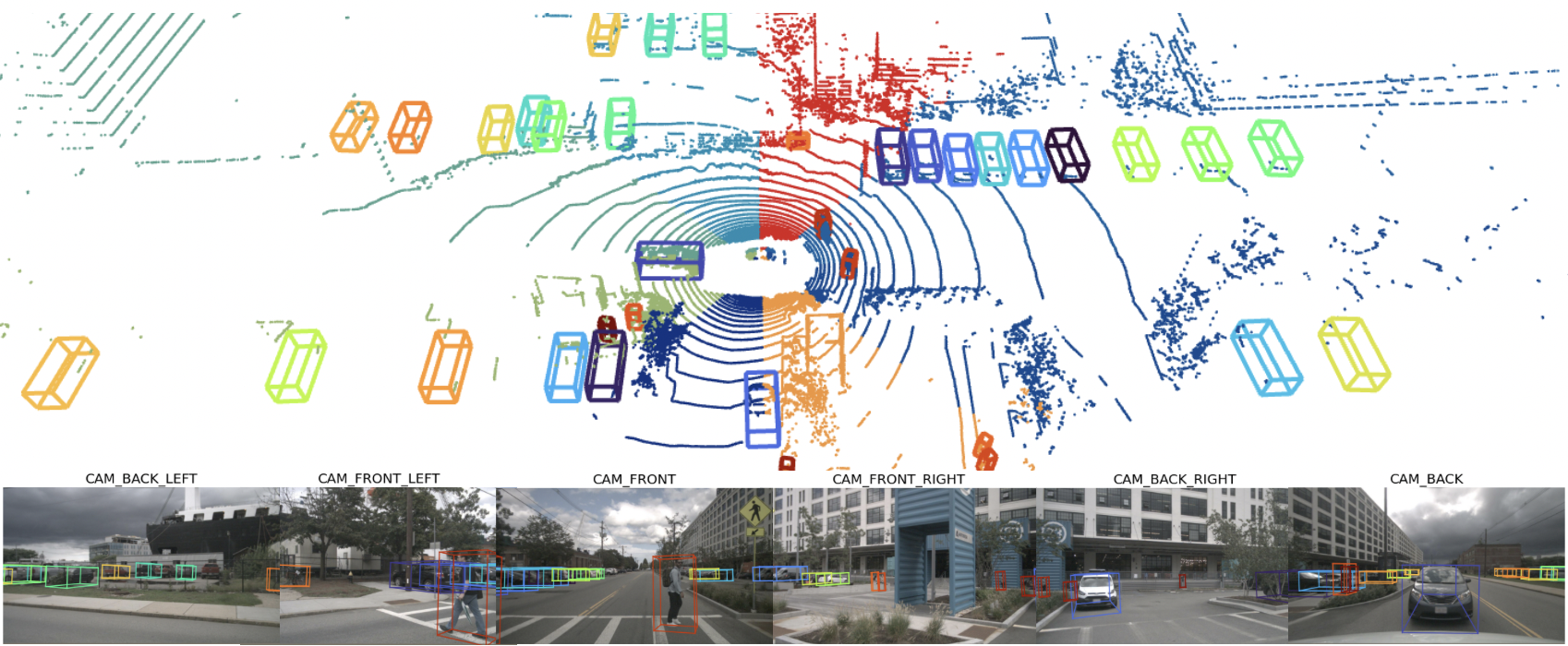
We compare the proposed model with both streaming and non-streaming models. These include LiDAR-only, camera-only, and fusion models. Moreover, the robustness of our model to missing camera images and camera-LiDAR miscalibration is studied and discussed. We also report ablation studies related to runtime, model design, and the effect of different image resolutions. Qualitative examples are demonstrated in Fig. 4 and 6.
V-A Detection Benchmark Results
Evaluated on the NuScenes test set, our 8-slice model achieves the state-of-the-art (SOTA) mAP for streaming models without using any past features (see Table I). This accuracy surpasses the 4-slice PolarStream [6] model, showing that even with more fragmentation and without access to past information, our model performs better for detection. For the test set, our model outperforms popular full-sweep detectors and baselines (both LiDAR-only and fusion-based ones). It is worthy noting that our results were obtained without using data augmentation in order to maintain cross-modal consistency. As shown in prior work [13, 2, 3], augmentation can significantly boost mAP.
| Model | Modality | Stream | mAP | Car | Ped | Bicycle |
| PointPillars [16] | PC | ✗ | 29.5 | 70.5 | 59.9 | 1.60 |
| ImVoxelNet [25] | RGB | ✗ | - | 51.8 | - | - |
| 3D-CVF [18] | PC+RGB | ✗ | 42.2 | 79.7 | 71.3 | - |
| MoCa [26] | PC+RGB | ✗ | 47.9 | 82.4 | 79.1 | 27.2 |
| CenterPointp [2] | PC | ✗ | 49.1 | 83.8 | 77.4 | 12.7 |
| Ours (all) | PC+RGB | ✗ | 57.6 | 83.8 | 80.9 | 51.6 |
| CenterPointp (8s) | PC | ✓ | 27.1 | 66.1 | 59.7 | 4.9 |
| Ours (8s) | PC+RGB | ✓ | 54.7 | 83.1 | 81.8 | 47.3 |
| Ours (16s) | PC+RGB | ✓ | 53.8 | 82.5 | 81.2 | 52.1 |
| Ours (32s) | PC+RGB | ✓ | 51.1 | 80.6 | 79.0 | 47.3 |
| Ours (8s) | PC+RGB | ✓ | 47.8 | 80.4 | 76.9 | 38.0 |
| pPillar-based. without the back camera image. | ||||||
V-A1 Comparisons with Streaming Models
As shown in Table II, our streaming mAP is on par or exceeds prior streaming methods without using memory mechanisms or features from past LiDAR slices. Current image features are able to effectively replace past LiDAR features and provide sufficient context for accurate streaming detection. Moreover, our 8-slice model performs better than models that take the whole scene or wider slices (4) as input. We believe 8-slice is generally a good middle ground between too few or too many slices. It is enough to reduce latency and still contains enough contextual information. As a baseline, we implement a streaming variant of a comparable and powerful LiDAR-only detector (Pillar-based CenterPointp [2]) by limiting its input to one slice during training and evaluation. As shown in Table II, our RGB representation was able to restore and surpass all lost accuracy due to streaming, when compared to the streaming CenterPointp. Even at detrimental heavy fragmentation (32 slices) our model increases mAP from 2.2 to 51.1. This 32-slice mAP exceeds that of the full-sweep CenterPointp shown in Table III. Also, our full-scan model was able to increase mAP for CenterPointp by 8.5, showing the benefit of our fusion mechanism even for full-scan models. Finally, maintaining mAP between all slicing scenarios shows that the image features provide valuable and stable context that can withstand point cloud fragmentation (see Fig. 1). Results of prior streaming models on NuScenes validation set were reported in [6].

V-A2 Comparisons with Non-streaming Models
Taking as input a fraction of the 3D scene, our model is able to detect objects even when heavily fragmented (for 8, 16, and 32 slices) with an accuracy higher than prior full-sweep models on 3D detection and a similar LiDAR-only detector (CenterPointp). As shown in Table III, without access to past information, mAP degrades significantly for the streaming CenterPoint. However, our proposed fusion method provides enough context to replenish an impoverished point cloud input. Most notable, our streaming models are able to improve the accuracy for small object detection, especially for the bicycle class. This is likely because: a) bicycles have a small point cloud footprint with inconsistent shapes compared to other objects like cars and pedestrians; and b) bicycle is a tail class on NuScenes [24]. For both reasons, it benefits greatly from semantically-rich image features.
V-A3 Robustness to missing images/few points
We experiment with training without the image from the back camera (which has a wider FoV than other cameras) and note that our mAP degrades only slightly for the critical car and pedestrian classes (the last row of Table III). This shows that our model is somewhat robust to missing camera images. This is shown qualitatively as well by visualizing accurate detections behind the ego-vehicle in Fig. 4. Moreover, at heavy fragmentation and with a limited number of points, our 32-slice model maintains high accuracy. These observations illustrate the benefit of decoupling the image and point streams for a robust complimentary multi-modal representation.
V-B On Calibration
Point-wise fusion models depend heavily on accurate camera-LiDAR calibration, which can be difficult to maintain during operation due to mechanical vibrations or thermal strains [17, 27]. This dependence comes from decorating points directly with image features or segmentation scores [10, 3, 28]. In contrast, our model’s decoupling of point/image encoding and its relatively sparse volumetric representation for image features lead to better robustness to small calibration errors. To study the effect of calibration error, we survey SOTA work on online self-calibration (traditional [29] and learning-based [27, 30, 31]) and find that they can bring the mean Euler angle error down to around and mean translation error to from the ground truth calibration depending on the level of noise.

To simulate the error, we follow prior work in self-calibration by uniformly sampling (within a range) a translation vector and Euler angles (producing a noisy rotation matrix). These noisy transformations are applied to the ground truth extrinsic matrix . We test on 4 thresholds within the expected error and on 2 worst case scenario errors at and . As shown in Fig. 5, even the calibration error can greatly change the pixel-point correspondence where small and critical objects like pedestrians are almost completely covered by road features. Such issues are exacerbated with distance. The work in [3] has shown that even with accurate calibration, false negatives in segmentation masks can be detrimental for models that use point-wise decoration with segmentation scores [10]. Point-wise features projected with noise would be deeply problematic. In contrast, our model shows robustness by maintaining strong performance at that noise level with only a 2.7 degradation in mAP. However, at very high noises, accuracy degrades indicating that image features do provide valuable context for streaming multi-modal detection. At all noise levels, our mAP performance remains higher than the full-scan LiDAR-only baseline [16].
| Module | GFLOPS | Runtime (ms) | Runtime/fp16 (ms) | mAP |
|---|---|---|---|---|
| Pts. + BEV Enc. + Multi-Head | 180.2 | 44.5 | 33.8 | 54.7 |
| Pts. + BEV Enc. + Single-Head | 161.6 | 27.4 | 18.2 | 54.7 |
| Above w/ cropping | 40.43 | 15.8 | 14.0 | 54.7 |
| 3D Convolutions | 715.7 | 157.6 | 61.6 | - |
| Above w/ cropping | 178.9 | 38.5 | 15.9 | - |
| Img Encoding (1600x900) | 126.5 | 28.9 | 14.8 | 54.7 |
| Above w/ (1200x675) | 71.6 | 17.2 | 11.7 | 53.9 |
| Above w/ (800x450) | 32.1 | 9.8 | 11.7 | 50.8 |
V-C On Parallelization
While prior streaming work can be more light-weight, our work facilitates faster runtimes by allowing better parallelization. This is accomplished by removing multiple sequential dependencies. First, in the proposed framework, point encoding does not depend on image features. Thus, encoding of both modalities can run in parallel. Second, our framework does not require past slice features which allows for processing slices in parallel as they arrive.
Considering the parallelism inherent in the proposed method and the fast frame rate of cameras, our streaming framework can be efficient in terms of the end-to-end runtime. For example, an AV can take advantage of this parallelism by maintaining our proposed 3D volumetric representation of the world and simply updating it as images arrive from cameras. In that case, the LiDAR-only stream only has to fetch the most up-to-date features from the image’s BEV representation. Thus the end-to-end runtime (starting from a point cloud slice in the input, and ending with detections in the output) of our 8-slice streaming model is only 15.8 ms with SOTA accuracy. Also, since our framework is fully convolutional, it benefits from the advances in neural network quantization and pruning [32]. Finally, this parallel streaming approach allows the computational burden of perception to be distributed along the scan instead of processing the whole scene at once, or in a sequence.
We study runtime and FLOPs of various components of our (8-slice) model on a Tesla V100 GPU and report the results in Table IV. A slice () can be covered by a single image based on the FoV of Nuscenes cameras () and contains about 30000 points. These values are used during runtime testing. Moreover, runtime is reported at full and half precision (fp16) since many latency-critical applications use fp16 to speed up inference and reduce storage requirements. Table IV shows the significant impact of our cropping operation on 3D convolutions (75% reduction in runtime and FLOPs) and on our LiDAR-only pipeline.
Our (8-slice) streaming framework is faster than all prior 8-slice streaming models. After adding for a 20 Hz LiDAR to collect a slice, prior work mostly runs at 37 frames per second (FPS) [6]. On the other hand, our framework runs at 45 Hz. If a slice arrives every , and processing by prior work takes about 20 ms [6], then the current slice has to wait until the previous one is processed. This is the pitfall of depending on past slices. In our case, multiple slices can be processed simultaneously, which can be exploited by accelerators like FPGAs or GPUs.
Our mAP gains are mainly from processing images. Image feature extraction is a process that is done anyway on most AV perception stacks. Image information is often indispensable, and we use a standard ResNet-50 backbone which is pre-trained on typical perception tasks. We study the effect of smaller image resolutions on the overall runtime. While images with smaller resolution lose some details, they still maintain high mAP at a much faster runtime, as shown in Table IV. Fp16 seems saturated at a certain low resolution. This implies that the overhead of operating at fp16 precision overcomes its benefits at lower resolutions.
VI Conclusion
This study proposes a multi-modal framework for 3D detection from streaming LiDAR point cloud data. To reduce latency in detection, our approach processes LiDAR slices as they come and expands their context using camera images. Parallel encoding and independence from past slices enable further reduction in latency using hardware accelerators, especially when coupled with our proposed cropping operation. The robustness of the proposed framework to small calibration errors, missing camera images, and heavily fragmented point clouds was studied and demonstrated. Our streaming framework is shown to outperform streaming as well as representative full-scan models in terms of detection accuracy on a challenging benchmark.
References
- [1] H. Caesar et al., “nuscenes: A multimodal dataset for autonomous driving,” in Proceedings of the IEEE/CVF conference on computer vision and pattern recognition, 2020, pp. 11 621–11 631.
- [2] T. Yin, X. Zhou, and P. Krahenbuhl, “Center-based 3d object detection and tracking,” in Proceedings of the IEEE/CVF Conference on Computer Vision and Pattern Recognition, 2021, pp. 11 784–11 793.
- [3] C. Wang et al., “Pointaugmenting: Cross-modal augmentation for 3d object detection,” in Proceedings of the IEEE/CVF Conference on Computer Vision and Pattern Recognition, 2021, pp. 11 794–11 803.
- [4] W. Han et al., “Streaming object detection for 3-d point clouds,” in European Conference on Computer Vision, 2020, pp. 423–441.
- [5] D. Frossard et al., “Strobe: Streaming object detection from lidar packets,” in Proceedings of the 2020 Conference on Robot Learning, ser. Proceedings of Machine Learning Research, vol. 155. PMLR, 16–18 Nov 2021, pp. 1174–1183.
- [6] Q. Chen, S. Vora, and O. Beijbom, “Polarstream: Streaming object detection and segmentation with polar pillars,” Advances in Neural Information Processing Systems, vol. 34, 2021.
- [7] Y. Sun et al., “Pointmoseg: Sparse tensor-based end-to-end moving-obstacle segmentation in 3-d lidar point clouds for autonomous driving,” IEEE Robotics and Automation Letters, vol. 6, no. 2, pp. 510–517, 2021.
- [8] M. Liang, B. Yang, S. Wang, and R. Urtasun, “Deep continuous fusion for multi-sensor 3d object detection,” in Proceedings of the European Conference on Computer Vision (ECCV), 2018, pp. 641–656.
- [9] T. Huang, Z. Liu, X. Chen, and X. Bai, “Epnet: Enhancing point features with image semantics for 3d object detection,” in European Conference on Computer Vision. Springer, 2020, pp. 35–52.
- [10] S. Vora et al., “Pointpainting: Sequential fusion for 3d object detection,” in Proceedings of the IEEE/CVF conference on computer vision and pattern recognition, 2020, pp. 4604–4612.
- [11] Z. Zhuang et al., “Perception-aware multi-sensor fusion for 3d lidar semantic segmentation,” in Proceedings of the IEEE/CVF International Conference on Computer Vision, 2021, pp. 16 280–16 290.
- [12] Y. Zhou and O. Tuzel, “Voxelnet: End-to-end learning for point cloud based 3d object detection,” in Proceedings of the IEEE conference on computer vision and pattern recognition, 2018, pp. 4490–4499.
- [13] Y. Yan, Y. Mao, and B. Li, “Second: Sparsely embedded convolutional detection,” Sensors, vol. 18, no. 10, p. 3337, 2018.
- [14] G. P. Meyer, A. Laddha, E. Kee, C. Vallespi-Gonzalez, and C. K. Wellington, “Lasernet: An efficient probabilistic 3d object detector for autonomous driving,” in Proceedings of the IEEE/CVF Conference on Computer Vision and Pattern Recognition, 2019, pp. 12 677–12 686.
- [15] L. Fan, X. Xiong, F. Wang, N. Wang, and Z. Zhang, “Rangedet: In defense of range view for lidar-based 3d object detection,” in Proceedings of the IEEE/CVF International Conference on Computer Vision, 2021, pp. 2918–2927.
- [16] A. H. Lang et al., “Pointpillars: Fast encoders for object detection from point clouds,” in Proceedings of the IEEE/CVF Conference on Computer Vision and Pattern Recognition, 2019, pp. 12 697–12 705.
- [17] Y. Cui et al., “Deep learning for image and point cloud fusion in autonomous driving: A review,” IEEE Transactions on Intelligent Transportation Systems, 2021.
- [18] J. H. Yoo et al., “3d-cvf: Generating joint camera and lidar features using cross-view spatial feature fusion for 3d object detection,” in European Conference on Computer Vision. Springer, 2020, pp. 720–736.
- [19] C. R. Qi, H. Su, K. Mo, and L. J. Guibas, “Pointnet: Deep learning on point sets for 3d classification and segmentation,” in Proceedings of the IEEE conference on computer vision and pattern recognition, 2017, pp. 652–660.
- [20] K. He, X. Zhang, S. Ren, and J. Sun, “Deep residual learning for image recognition,” in Proceedings of the IEEE conference on computer vision and pattern recognition, 2016, pp. 770–778.
- [21] T.-Y. Lin, P. Dollár, R. Girshick, K. He, B. Hariharan, and S. Belongie, “Feature pyramid networks for object detection,” in Proceedings of the IEEE conference on computer vision and pattern recognition, 2017, pp. 2117–2125.
- [22] S. Ioffe and C. Szegedy, “Batch normalization: Accelerating deep network training by reducing internal covariate shift,” in International conference on machine learning. PMLR, 2015, pp. 448–456.
- [23] K. Chen et al., “Hybrid task cascade for instance segmentation,” in Proceedings of the IEEE/CVF Conference on Computer Vision and Pattern Recognition, 2019, pp. 4974–4983.
- [24] B. Zhu, Z. Jiang, X. Zhou, Z. Li, and G. Yu, “Class-balanced grouping and sampling for point cloud 3d object detection,” arXiv preprint arXiv:1908.09492, 2019.
- [25] D. Rukhovich, A. Vorontsova, and A. Konushin, “Imvoxelnet: Image to voxels projection for monocular and multi-view general-purpose 3d object detection,” in Proceedings of the IEEE/CVF Winter Conference on Applications of Computer Vision, 2022, pp. 2397–2406.
- [26] W. Zhang et al., “Exploring data augmentation for multi-modality 3d object detection,” arXiv preprint arXiv:2012.12741, 2020.
- [27] K. Yuan, Z. Guo, and Z. J. Wang, “Rggnet: Tolerance aware lidar-camera online calibration with geometric deep learning and generative model,” IEEE Robotics and Automation Letters, vol. 5, no. 4, pp. 6956–6963, 2020.
- [28] V. A. Sindagi, Y. Zhou, and O. Tuzel, “Mvx-net: Multimodal voxelnet for 3d object detection,” in 2019 International Conference on Robotics and Automation (ICRA). IEEE, 2019, pp. 7276–7282.
- [29] Z. Taylor and J. Nieto, “Motion-based calibration of multimodal sensor extrinsics and timing offset estimation,” IEEE Transactions on Robotics, vol. 32, no. 5, pp. 1215–1229, 2016.
- [30] X. Lv et al., “Lccnet: Lidar and camera self-calibration using cost volume network,” in Proceedings of the IEEE/CVF Conference on Computer Vision and Pattern Recognition, 2021, pp. 2894–2901.
- [31] Z. Liu, H. Tang, S. Zhu, and S. Han, “Semalign: Annotation-free camera-lidar calibration with semantic alignment loss,” in 2021 IEEE/RSJ International Conference on Intelligent Robots and Systems (IROS). IEEE, 2021, pp. 8845–8851.
- [32] J. Martinez et al., “Permute, quantize, and fine-tune: Efficient compression of neural networks,” in Proceedings of the IEEE/CVF Conference on Computer Vision and Pattern Recognition, 2021, pp. 15 699–15 708.