Unsupervised Learning of 3D Scene Flow with 3D Odometry Assistance Thanks: *This work was supported in part by the Natural Science Foundation of China under Grant 62073222, Grant U21A20480, and Grant U1913204; in part by the Science and Technology Commission of Shanghai Municipality under Grant 21511101900; and in part by the Open Research Projects of Zhejiang Laboratory under Grant 2022NB0AB01. The first two authors contributed equally. Corresponding Author: Hesheng Wang.Thanks: G. Wang, Z. Feng, and H. Wang are with Department of Automation, Key Laboratory of System Control and Information Processing of Ministry of Education, Key Laboratory of Marine Intelligent Equipment and System of Ministry of Education, Shanghai Engineering Research Center of Intelligent Control and Management, Shanghai Jiao Tong University, Shanghai 200240, China. Thanks: C. Jiang is with Engineering Research Center of Intelligent Control for Underground Space, Ministry of Education, School of Information and Control Engineering, Advanced Robotics Research Center, China University of Mining and Technology, Xuzhou 221116, China.

Attentive cost volume is introduced in [8] for calculating the cost volume of two point clouds. The cost volume $CV_{self}(p_{i})$ obtained by this method is without occlusion perception between point cloud $P$ and point cloud $Q$.

First, the position information between $p_{i}$ and its $K_{1}$ nearest neighbors $q_{k}$ ($k=1,2,...,K_{1}$) in point cloud $Q$ is encoded by the Eq. (2):

Then, the encoded feature $f_{q2p}(p_{i,k})$ between $p_{i}$ and its $K_{1}$ nearest neighbors $q_{k}$ ($k=1,2,...,K_{1}$) is calculated by the Eq. (3):

where $f_{p_{i}}$ is the encoded feature of $p_{i}$, and $f_{q_{k}}$ is the encoded feature of $q_{k}$. For point $p_{i}$, when calculating the information of feature matching, both the distance and the feature similarity between $p_{i}$ and its $K_{1}$ nearest neighbors have influence on the aggregation weights. Therefore, the weights $w_{q2p}(i,k)$ for $f_{q2p}(p_{i,k})$ is calculated as follows:

The cost volume $cost_{self}(p_{i})$ between $p_{i}$ and its $K_{1}$ nearest neighbors in point cloud $Q$ is represented as:

where $\odot$ means dot product. $p_{k}$ is the $k$-th point in the $K_{1}$ nearest neighbors of $p_{i}$.

Next, the feature aggregation in point cloud $P$ is performed to expand the received fields of the cost volume [34]. The weights $w_{p2p}(i,k)$ of $p_{i}$ and its $K_{2}$ nearest neighbors $p_{k}$ ($k=1,2,...,K_{2}$) in $P$ is calculated by using the similar method shown as Eq. (4). Finally, the attentive cost volume $CV_{self}(p_{i})$ is calculated by the formula as follows:

The feature $f_{O}$ of the occlusion mask is calculated by using the attentive cost volume. $f_{O}$ is passed through an FC layer and sigmoid activation function to obtain the occlusion mask $O$. The mask is a weight matrix whose element value is from 0 to 1. The value represents the probability that the point is a non-occluded point. The formula is:

When a point $p_{i}$ is occluded, its cost volume $CV_{self}(p_{i})$ is unreliable. The cost volume of this point should be guided by its $K$ nearest neighbors. Therefore, the final cost volume $CV_{o}(p_{i})$ with occlusion perception is designed as:

where the $N(p_{i})$ are the $K$ nearest neighbors of point $p_{i}$. $O(p_{i})$ is the occlusion mask value of $p_{i}$. $CV_{local}(p_{i})$ is the cost volume guided by $N(p_{i})$. As shown in Eq. (9), we focus on that the $CV_{self}(p_{i})$ has a higher contribution for non-occluded points, while the $CV_{local}(p_{i})$ has a higher contribution for occluded points.

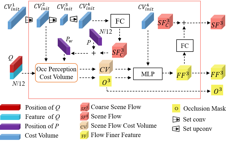
The initial cost volume $CV_{init}^{1}$ is sampled to get ${CV}_{init}^{2}$, ${CV}_{init}^{2}$ is sampled to get ${CV}_{init}^{3}$, and the ${CV}_{init}^{3}$ is up-sampled to get ${CV}_{init}^{4}$. An FC layer is used to generate ${SF}_{C}^{3}$ which is the initial estimation of the scene flow. The formula is:

The predicted point cloud $P_{w}$ is obtained by adding ${SF}_{C}^{3}$ to the point cloud $P$. The point cloud $Q$, the features of $Q$, $P_{w}$, and ${CV}_{init}^{2}$ are input into the occlusion perception cost volume to obtain the coarse estimated mask $O^{3}$ and the cost volume $CV$. The MLP is used to generate the coarse flow feature ${FF}^{3}$. The formula is:

Finally, the output coarse scene flow ${SF}^{3}$ is:

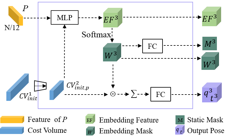
The initial cost volume $CV_{init}^{1}$ is sampled to get $CV_{init,p}^{2}=\{cv_{i,p}^{2}|cv_{i,p}^{2}\in\mathbb{R}^{c}\}$. The MLP is used to generate the embedding feature ${EF}^{3}$. For the odometry task, ego-motion is affected by moving objects in the real world. PWCLO-Net [29] proposes a embedding mask $W$ to weight the embedding features of dynamic and static points. Because the $w^{3}$ is on the feature dimension of the embedding feature, an FC layer is used to obtain the static mask $M^{3}$. The formula is:

We use $W^{3}$ as the weight to calculate the $feat_{qt}$ which is the feature that contains information about the pose transformation. The formual is:

Finally, the coarse estimation of quaternion $q^{3}$ and translation vector $t^{3}$ is:

Set upconv layer is adapted to propagate embedding features $EF^{l+1}=\{ef_{i}|ef_{i}\in\mathbb{R}^{c}\}_{i=1}^{N^{l+1}}$, flow feature $FF^{l+1}=\{ff_{i}|ff_{i}\in\mathbb{R}^{c}\}_{i=1}^{N^{l+1}}$, and embedding mask $W^{l+1}=\{w_{i}|w_{i}\in\mathbb{R}^{c}\}_{i=1}^{N^{l+1}}$ from ($l$+1)-th level to $l$-th level. $EF^{l}_{up}=\{ef_{i}|ef_{i}\in\mathbb{R}^{c}\}_{i=1}^{N^{l}}$, flow feature $FF^{l}_{up}=\{ff_{i}|ff_{i}\in\mathbb{R}^{c}\}_{i=1}^{N^{l}}$, and embedding mask $W^{l}_{up}=\{w_{i}|w_{i}\in\mathbb{R}^{c}\}_{i=1}^{N^{l}}$ are obtained by the set upconv layer.

Because the number of points in the ($l$+1)-th level is less than that in the $l$-th level. The interpolation up-sampling method based on three nearest neighbors (Three-NN) [33] is used to up-sample the static mask $M^{l+1}$, occlusion mask $O^{l+1}$, and scene flow $SF^{l+1}$ to obtain the mask $M^{l}_{up}$, $O^{l}_{up}$, and $SF^{l}_{up}$ of the $l$-th level.

In the classical coarse-to-fine scene flow estimation method, the warp operation is the key to scene flow refinement. To get more accurate predicited point clouds, the point cloud warping layer with occlusion and static mask shown in Fig. 6 is designed. The warp operation of point clouds means that scene flow or pose estimated at the ($l$+1)-th level are applied to warp source point cloud to generate predicted point cloud $P^{l}_{warp}$. $P^{l}_{w,pose}$ and $P^{l}_{w,sf}$ denote predicted point clouds obtained using pose estimation and scene flow estimation, respectively. The formula to calculate $P^{l}_{w,pose}$ and $P^{l}_{w,sf}$ is:

where Eq. (16) means quaternion $q^{l+1}$ and translation vector $t^{l+1}$ are applied to warp $P^{l}$ to generate $P^{l}_{w,pose}=\{p^{l}_{pose,i}|p^{l}_{pose,i}\in\mathbb{R}^{3}\}$. Eq. (17) means $SF^{l}_{up}=\{sf^{l}_{i,up}|sf^{l}_{i,up}\in\mathbb{R}^{3}\}$ is applied to warp $P^{l}$ to generate $P^{l}_{w,sf}=\{p^{l}_{sf,i}|p^{l}_{sf,i}\in\mathbb{R}^{3}\}$.

Static points are more accurate for pose estimation, while dynamic points or non-occluded points are more accurate for scene flow estimation. The mask $H^{l}_{w}=\{h^{l}_{i}|h^{l}_{i}\in\mathbb{R}^{1}\}$ used to calculate the weights of $P^{l}_{w,pose}$ and $P^{l}_{w,sf}$ is calculated as follows:

Finally, the predicted point cloud $P_{warp}^{l}$ at the $l$-th level is represented as:

$EF^{l}_{up}$, $CV_{self}$, and the feature of $P^{l}$ are concatenated and input into an MLP to produce refined $EF^{l}$. Then, $M^{l}_{up}$, $EF^{l}$, and the feature of $P^{l}$ are concatenated and input into an MLP to produce refined $W^{l}$. The $feat_{qt}^{l}$ which contains the residual information of pose transformation can be obtained from embedding feature $EF^{l}$ and embedding mask $W^{l}$ using the Eq. (14).

Then, the residual values $\Delta q$ and $\Delta t$ can be obtained from $feat_{qt}^{l}$ using the Eq. (15). In the pose estimation at the $l$-th level, the formula for calculating the refined $q^{l}$ and $t^{l}$ is:

Some objects are not continuously visible between consecutive frames due to occlusion. The occlusion mask $O$ is used to distinguish occluded points and non-occluded points in point clouds.

When estimating the scene flow, to weaken the influence of occluded points, the information of the occlusion mask is included in the formula for calculating flow feature $FF^{l}$:

where $F^{l}$ is the feature of point cloud $P^{l}$. Finally, the formulas for residual flow $\Delta SF^{l}$ and scene flow $SF^{l}$ estimation are:

The predicted scene flow $SF^{l}=\{sf^{l}_{i}|sf_{i}\in\mathbb{R}^{3}\}_{i=1}^{N^{l}}$ at the $l$-th level is added to point cloud $P^{l}$ of the first frame to get the warped point cloud $P_{w}^{l}=\{p_{w,i}^{l}|p_{w,i}^{l}\in\mathbb{R}^{3}\}_{i=1}^{N^{l}}$ which is expected as close to the target point cloud $Q^{l}=\{q_{i}^{l}|q_{i}^{l}\in\mathbb{R}^{3}\}_{i=1}^{N^{l}}$ as possible. The formula is:

where $||\cdot||_{2}$ means $l_{2}$ norm.

To ensure that the scene flow predicted in the local area is smooth, we need to introduce a smooth regularization constraint. The scene flow of the point $p_{i}^{l}$ can be constrained by the scene flow of its $K$ neighbors. The formula is:

where $N(p_{i}^{l})$ is $K$ nearest neighbors of $p_{i}$. $|N(p_{i}^{l})|$ is the the number of points in the local region $N(p_{i}^{l})$.

The shape characteristic of a certain point in a point cloud is represented by a Laplace vector as follows:

where the $v(p_{i})$ is the Laplacian characteristic of point $p_{i}$.

The predicted point cloud $P_{w}^{l}$ and the target point cloud $Q^{l}$ have similar local shape characteristics at corresponding points. The Eq. (26) is used to calculate the Laplacian characteristic $v(q_{i}^{l})$ of $q_{i}^{l}$ and the Laplacian characteristic $v(p_{w,i}^{l})$ of $p_{w,i}^{l}$. Then, is used to obtain the Laplacian characteristic $v(q_{inter}^{l})$ of $q_{inter}^{l}$ is obtained by the inverse distance-based interpolation from $q_{i}^{l}$. The $q_{inter}^{l}$ is the corresponding point of $p_{w,i}^{l}$ in $P_{w}^{l}$. The loss formula is:

In summary, the scene flow unsupervised loss formula is:

where $\alpha_{l}$ denotes the weight for each pyramid level. $\sigma_{C}$, $\sigma_{S}$, and $\sigma_{L}$ denote the weight for these three unsupervised losses, respectively.

The loss function of the network consists of two parts, the scene flow unsupervised loss and the pose supervised loss. In the scene flow unsupervised loss, the weights of each layer loss are ${\alpha_{0}}=0.02$, ${\alpha_{1}}=0.04$, ${\alpha_{2}}=0.08$, and ${\alpha_{3}}=0.16$. The weights for three scene flow unsupervised loss are $\sigma_{C}=1.0$, $\sigma_{S}=1.0$, and $\sigma_{L}=0.3$. In the pose supervised loss, the weights of each layer loss are ${\lambda_{0}}=0.2$, ${\lambda_{1}}=0.4$, ${\lambda_{2}}=0.8$, and ${\lambda_{3}}=1.6$. In the total loss, the weights are $\mu_{sf}=1$ and $\mu_{p}=1$. We divide the training process into three stages: training only the odometry network until convergence, training only the scene flow network until convergence, and training with both networks together until convergence.

As shown in Fig. 1, the number of the points input to the network is $4N=8192$. The number of downsampling point cloud in each layer are $N^{1}=N=2048$, $N^{2}=\frac{1}{2}N=1024$, $N^{3}=\frac{1}{8}N=256$, and $N^{4}=\frac{1}{32}N=64$ respectively.

The environment for the experimental configuration is GeForce RTX 3090 GPU with CUDA = 11.3 and PyTorch = 1.10.0. The optimizer is Adam [39] with ${\beta_{1}}=0.9$ and ${\beta_{2}}=0.999$. The initial learning rate is 0.001. The learning rate will decay exponentially with a decay step of 13 epochs and a decay rate of 0.7. The batch size is 8.

FlyingThings3D (FT3D) [12] dataset provides more than 20,000 pairs of synthesized point clouds and corresponding scene flow annotations. FT3D is often used to train scene flow estimation models due to its large data with scene flow annotations. However, there are significant differences between the synthesized dataset and the real-world dataset, which results in models trained on the synthesized dataset not being well adapted to the real-world scene. The KITTI Odometry (K-OD) dataset [40] is obtained by using Velodyne 64-beam LiDAR. It provides 11 sequences, each of which contains LiDAR point clouds and pose ground truth. The pose ground truth is used to supervise the odometry training. Our method learns 3D scene flow on continuous frames of LiDAR point clouds of sequences 00-06 in an unsupervised way. The ground points of each frame of point cloud are removed.

• $\bullet$

  K-SF-142. KITTI Scene Flow 2015 (K-SF) [41, 42] consists of 200 training scenes and 200 test scenes which are used for evaluations of RGB stereo-based methods. K-SF-142 consists of 142 pairs in K-SF training scenes. PointPWC-Net [11] selected these 142 pairs for evaluation. These point clouds and ground truth flow are generated by projecting annotated disparity maps and optical flow to 3D. We also choose these 142 pairs as our test dataset. The ground points are removed from the point clouds of evaluation datasets like previous methods [15, 11, 13, 35]. For the fine-tuning experiment, we divide them into 100 training samples and 42 test samples.

• $\bullet$

  lidarKITTI. lidarKITTI [43] is a real-world dataset collected by using a Velodyne 64-beam LiDAR. There are the same 142 pairs as K-SF-142. The dataset is obtained by projecting the point cloud onto the image plane and assigning it annotated 3D scene flow. In the dataset, the points of two input frames do not correspond directly and have a typical LiDAR sensor sampling pattern. For the fine-tuning experiment, we use 100 pairs for fine-tuning training and 42 pairs for testing.

Because the K-SF-142 dataset is synthesised from optical flow and disparity map, the points in the point clouds of two consecutive frames correspond point by point in the K-SF-142 dataset. The previous method selects 8192 points at random in each of the two frames so that the selected points do not correspond point by point. The lidarKITTI is the raw LiDAR point cloud dataset, where the points in the point clouds do not correspond point by point, and the data suffers noise from the LiDAR sensor. Therefore, the lidarKITTI dataset is more challenging.

References

- [1] A. Behl, O. Hosseini Jafari, S. Karthik Mustikovela, H. Abu Alhaija, C. Rother, and A. Geiger, “Bounding boxes, segmentations and object coordinates: How important is recognition for 3d scene flow estimation in autonomous driving scenarios?” in Proc. IEEE Int. Conf. Comput. Vis. (ICCV), 2017, pp. 2574–2583.
- [2] Z. Cao, A. Kar, C. Hane, and J. Malik, “Learning independent object motion from unlabelled stereoscopic videos,” in Proc. IEEE Conf. Comput. Vis. Pattern Recognit. (CVPR), 2019, pp. 5594–5603.
- [3] S. Wang, Y. Sun, C. Liu, and M. Liu, “Pointtracknet: An end-to-end network for 3-d object detection and tracking from point clouds,” IEEE Robot. Autom., vol. 5, no. 2, pp. 3206–3212, 2020.
- [4] G. Wang, C. Peng, J. Zhang, and H. Wang, “Interactive multi-scale fusion of 2d and 3d features for multi-object tracking,” arXiv preprint arXiv:2203.16268, 2022.
- [5] X. Liu, M. Yan, and J. Bohg, “Meteornet: Deep learning on dynamic 3d point cloud sequences,” in Proc. IEEE Int. Conf. Comput. Vis. (ICCV), 2019, pp. 9246–9255.
- [6] Z. Lv, K. Kim, A. Troccoli, D. Sun, J. M. Rehg, and J. Kautz, “Learning rigidity in dynamic scenes with a moving camera for 3d motion field estimation,” in Proc. Eur. Conf. Comput. Vis. (ECCV), 2018, pp. 468–484.
- [7] W.-C. Ma, S. Wang, R. Hu, Y. Xiong, and R. Urtasun, “Deep rigid instance scene flow,” in Proc. IEEE Conf. Comput. Vis. Pattern Recognit. (CVPR), 2019, pp. 3614–3622.
- [8] G. Wang, X. Wu, Z. Liu, and H. Wang, “Hierarchical attention learning of scene flow in 3d point clouds,” IEEE Trans. Image Process., vol. 30, pp. 5168–5181, 2021.
- [9] X. Gu, Y. Wang, C. Wu, Y. J. Lee, and P. Wang, “Hplflownet: Hierarchical permutohedral lattice flownet for scene flow estimation on large-scale point clouds,” in Proc. IEEE Conf. Comput. Vis. Pattern Recognit. (CVPR), 2019, pp. 3254–3263.
- [10] X. Liu, C. R. Qi, and L. J. Guibas, “Flownet3d: Learning scene flow in 3d point clouds,” in Proc. IEEE Conf. Comput. Vis. Pattern Recognit. (CVPR), 2019, pp. 529–537.
- [11] W. Wu, Z. Y. Wang, Z. Li, W. Liu, and L. Fuxin, “Pointpwc-net: Cost volume on point clouds for (self-)supervised scene flow estimation,” in Proc. Eur. Conf. Comput. Vis. (ECCV). Springer, 2020, pp. 88–107.
- [12] N. Mayer, E. Ilg, P. Hausser, P. Fischer, D. Cremers, A. Dosovitskiy, and T. Brox, “A large dataset to train convolutional networks for disparity, optical flow, and scene flow estimation,” in Proc. IEEE Conf. Comput. Vis. Pattern Recognit. (CVPR), June 2016.
- [13] H. Mittal, B. Okorn, and D. Held, “Just go with the flow: Self-supervised scene flow estimation,” in Proc. IEEE Conf. Comput. Vis. Pattern Recognit. (CVPR), 2020, pp. 11 177–11 185.
- [14] G. Wang, C. Jiang, Z. Shen, Y. Miao, and H. Wang, “Sfgan: Unsupervised generative adversarial learning of 3d scene flow from the 3d scene self,” Adv. Intell. Syst., p. 2100197, 2021.
- [15] I. Tishchenko, S. Lombardi, M. R. Oswald, and M. Pollefeys, “Self-Supervised Learning of Non-Rigid Residual Flow and Ego-Motion,” in Int. Conf. 3D Vis. (3DV), 2020, pp. 150–159.
- [16] S. A. Baur, D. J. Emmerichs, F. Moosmann, P. Pinggera, B. Ommer, and A. Geiger, “Slim: Self-supervised lidar scene flow and motion segmentation,” in Proc. IEEE Conf. Comput. Vis. Pattern Recognit. (CVPR), 2021, pp. 13 126–13 136.
- [17] Z. Teed and J. Deng, “Raft: Recurrent all-pairs field transforms for optical flow,” in Proc. Eur. Conf. Comput. Vis. (ECCV). Springer, 2020, pp. 402–419.
- [18] X. Liu, C. R. Qi, and L. J. Guibas, “Flownet3d: Learning scene flow in 3d point clouds,” in Proc. IEEE Conf. Comput. Vis. Pattern Recognit. (CVPR), 2019, pp. 529–537.
- [19] G. Puy, A. Boulch, and R. Marlet, “Flot: Scene flow on point clouds guided by optimal transport,” in Proc. Eur. Conf. Comput. Vis. (ECCV). Springer, 2020, pp. 527–544.
- [20] G. Wang, Y. Hu, X. Wu, and H. Wang, “Residual 3d scene flow learning with context-aware feature extraction,” arXiv preprint arXiv:2109.04685, 2021.
- [21] Z. Gojcic, O. Litany, A. Wieser, L. J. Guibas, and T. Birdal, “Weakly supervised learning of rigid 3d scene flow,” in Proc. IEEE Conf. Comput. Vis. Pattern Recognit. (CVPR), June 2021, pp. 5692–5703.
- [22] B. Ouyang and D. Raviv, “Occlusion guided self-supervised scene flow estimation on 3d point clouds,” in Int. Conf. 3D Vis. (3DV). IEEE, 2021, pp. 782–791.
- [23] Z. Jin, Y. Lei, N. Akhtar, H. Li, and M. Hayat, “Deformation and correspondence aware unsupervised synthetic-to-real scene flow estimation for point clouds,” in Proc. IEEE Conf. Comput. Vis. Pattern Recognit. (CVPR), 2022, pp. 7233–7243.
- [24] G. Wang, Y. Hu, Z. Liu, Y. Zhou, M. Tomizuka, W. Zhan, and H. Wang, “What matters for 3d scene flow network,” Proc. Eur. Conf. Comput. Vis. (ECCV), 2022.
- [25] C. Zheng, Y. Lyu, M. Li, and Z. Zhang, “Lodonet: A deep neural network with 2d keypoint matching for 3d lidar odometry estimation,” in Proc. ACM Int. Conf. Multimed., 2020, pp. 2391–2399.
- [26] W. Wang, M. R. U. Saputra, P. Zhao, P. Gusmao, B. Yang, C. Chen, A. Markham, and N. Trigoni, “Deeppco: End-to-end point cloud odometry through deep parallel neural network,” in IEEE/RSJ Int. Conf. Intell. Robots. Syst. (IROS), 2019, pp. 3248–3254.
- [27] Q. Li, S. Chen, C. Wang, X. Li, C. Wen, M. Cheng, and J. Li, “Lo-net: Deep real-time lidar odometry,” in Proc. IEEE Conf. Comput. Vis. Pattern Recognit. (CVPR), 2019, pp. 8473–8482.
- [28] M. Velas, M. Spanel, M. Hradis, and A. Herout, “Cnn for imu assisted odometry estimation using velodyne lidar,” in IEEE Int. Conf. Auton. Robot Syst. Competitions. (ICARSC), 2018, pp. 71–77.
- [29] G. Wang, X. Wu, Z. Liu, and H. Wang, “Pwclo-net: Deep lidar odometry in 3d point clouds using hierarchical embedding mask optimization,” in Proc. IEEE Conf. Comput. Vis. Pattern Recognit. (CVPR), 2021, pp. 15 910–15 919.
- [30] G. Wang, X. Wu, S. Jiang, Z. Liu, and H. Wang, “Efficient 3d deep lidar odometry,” arXiv preprint arXiv:2111.02135, 2021.
- [31] K. Fischer, M. Simon, F. Olsner, S. Milz, H.-M. Groß, and P. Mader, “Stickypillars: Robust and efficient feature matching on point clouds using graph neural networks,” in Proc. IEEE Conf. Comput. Vis. Pattern Recognit. (CVPR), 2021, pp. 313–323.
- [32] S. Chopra, R. Hadsell, and Y. LeCun, “Learning a similarity metric discriminatively, with application to face verification,” in Proc. IEEE Conf. Comput. Vis. Pattern Recognit. (CVPR), vol. 1, 2005, pp. 539–546.
- [33] C. R. Qi, L. Yi, H. Su, and L. J. Guibas, “Pointnet++: Deep hierarchical feature learning on point sets in a metric space,” Proc. Adv. Neural Inf. Process. Syst., vol. 30, 2017.
- [34] Q. Hu, B. Yang, L. Xie, S. Rosa, Y. Guo, Z. Wang, N. Trigoni, and A. Markham, “Randla-net: Efficient semantic segmentation of large-scale point clouds,” in Proc. IEEE Conf. Comput. Vis. Pattern Recognit. (CVPR), 2020, pp. 11 108–11 117.
- [35] J. K. Pontes, J. Hays, and S. Lucey, “Scene flow from point clouds with or without learning,” in Int. Conf. 3D Vis. (3DV). IEEE, 2020, pp. 261–270.
- [36] P. J. Besl and N. D. McKay, “Method for registration of 3-d shapes,” in Sensor fusion IV: control paradigms and data structures, vol. 1611, 1992, pp. 586–606.
- [37] Q.-Y. Zhou, J. Park, and V. Koltun, “Fast global registration,” in Proc. Eur. Conf. Comput. Vis. (ECCV). Springer, 2016, pp. 766–782.
- [38] A. Myronenko and X. Song, “Point set registration: Coherent point drift,” IEEE Trans. Pattern Anal. Mach. Intell. (PAMI), vol. 32, no. 12, pp. 2262–2275, 2010.
- [39] D. P. Kingma and J. Ba, “Adam: A method for stochastic optimization,” arXiv preprint arXiv:1412.6980, 2014.
- [40] A. Geiger, P. Lenz, C. Stiller, and R. Urtasun, “Vision meets robotics: The kitti dataset,” Int. J. Robot. Res., vol. 32, no. 11, pp. 1231–1237, 2013.
- [41] M. Menze, C. Heipke, and A. Geiger, “Joint 3d estimation of vehicles and scene flow,” ISPRS Workshop on Image Sequence Analysis (ISA)., pp. 427–434, 2015.
- [42] M. Menze, C. Heipke, and A. Geiger, “Object scene flow,” ISPRS J. Photogram. Remote Sens. (JPRS), vol. 140, pp. 60–76, 2018.
- [43] A. Geiger, P. Lenz, and R. Urtasun, “Are we ready for autonomous driving? the kitti vision benchmark suite,” in Proc. IEEE Conf. Comput. Vis. Pattern Recognit. (CVPR), 2012, pp. 3354–3361.
![[Uncaptioned image]](2209.04945v1/Guangming.png) |
Guangming Wang received the B.S. degree from Department of Automation from Central South University, Changsha, China, in 2018. He is currently pursuing the Ph.D. degree in Control Science and Engineering with Shanghai Jiao Tong University. His current research interests include SLAM and computer vision, in particular, 3D scene flow estimation and LiDAR odometry. |
![[Uncaptioned image]](2209.04945v1/work_fzh2.jpg) |
Zhiheng Feng received the B.S. degree from Department of Automation from Shanghai Jiao Tong University, Shanghai, China, in 2022. His current research interests include SLAM and computer vision, in particular, 3D scene flow estimation and LiDAR odometry. |
![[Uncaptioned image]](2209.04945v1/jck_monochrome.jpg) |
Chaokang Jiang received the B.S. degree from the Department of Engineering, Jingdezhen Ceramic Institute College of Technology and Art, Jingdezhen, China, in 2020. He is currently pursuing the M.E. degree in control science and engineering with China University of Mining and Technology. His current research interests include SLAM and computer vision. |
![[Uncaptioned image]](2209.04945v1/hesheng.png) |
Hesheng Wang (SM’15) received the B.Eng. degree in electrical engineering from the Harbin Institute of Technology, Harbin, China, in 2002, and the M.Phil. and Ph.D. degrees in automation and computer-aided engineering from The Chinese University of Hong Kong, Hong Kong, in 2004 and 2007, respectively. He is currently a Professor with the Department of Automation, Shanghai Jiao Tong University, Shanghai, China. His current research interests include visual servoing, service robot, computer vision, and autonomous driving. Dr. Wang is an Associate Editor of IEEE Transactions on Automation Science and Engineering, IEEE Robotics and Automation Letters, Assembly Automation and the International Journal of Humanoid Robotics, a Technical Editor of the IEEE/ASME Transactions on Mechatronics, an Editor of Conference Editorial Board (CEB) of IEEE Robotics and Automation Society. He served as an Associate Editor of the IEEE Transactions on Robotics from 2015 to 2019. He was the General Chair of IEEE ROBIO 2022 and IEEE RCAR 2016, and the Program Chair of the IEEE ROBIO 2014 and IEEE/ASME AIM 2019. He will be the General Chair of IEEE/RSJ IROS 2025. |