Revisiting second-order optimality conditions for equality-constrained minimization problem

We consider the optimization problem with equality constraints :

defined by the objective function $f$ and the vector function $g=(g_{1},\cdots,g_{m}),\,m\leq n,$ for the constraints. We suppose that $f$ and $g$ are $C^{2}$ differentiable functions defined on $\mathbb{R}^{n}.$ ¹¹ 1 In the same way, we could consider that the functions $f$ and $g$ are defined on an open set $\Omega\subset\mathbb{R}^{n},\,\Omega\neq\emptyset.$

We suppose that $0\in\mathbb{R}^{m}$ is a regular value of $g$, i.e. the Jacobian $Jg(x)$ is full rank for every $x\in g^{-1}(\{0\}).$ Thus, $\mathcal{M}_{g}=g^{-1}(\{0\})=\{x\in\mathbb{R}^{n}\,|\,g(x)=0\}$ is a closed embedded $(n-m)$-dimensional submanifold of $\mathbb{R}^{n},$ and we know that, for every $x\in\mathcal{M}_{g},$ the tangent space $T_{x}\mathcal{M}_{g}$ at $x$ to $\mathcal{M}_{g}$ is equal to $\textrm{Ker}(Jg(x)).$

We recall the classical first-order and second-order optimality conditions for the problem (1) (see  [3] and  [4]).

If the point $x^{*}\in\mathcal{M}_{g}$ is a local minimum of (1), the first-order necessary conditions are given by

where $\nabla f(x^{*}),\nabla g_{i}(x^{*}),i=1,\ldots,m,$ are the gradients of $f$ and $g_{i}$ at $x^{*}$, $Jg(x^{*})$ the Jacobian matrix of $g$ at $x^{*},$ and $\lambda^{*}=(\lambda_{1}^{*},\cdots,\lambda_{m}^{*})\in\mathbb{R}^{m}$ the Lagrange multipliers vector.

Equation (2) says that the orthogonal of the tangent spaces $T_{x^{*}}\mathcal{M}_{f,x^{*}}$ and $T_{x^{*}}\mathcal{M}_{g}$ at $x^{*}$ satisfy the inclusion

or equivalently

Notice that for $m=1,$ the tangent spaces at $x^{*}$ are equal.

By introducing the Lagrangian function $L(x,\lambda)$ associated to the constrained optimization problem (1)

the conditions (2) are given by

where $\nabla_{x}$ is the gradient of $L$ with respect to $x.$

The second-order necessary conditions are the following (see  [3] and  [4]) :

with $\nabla^{2}f(x^{*})$ and $\nabla^{2}g_{i}(x^{*})$ the Hessian matrices of $f$ and $g_{i}$ at $x^{*},$ and supposing that first-order conditions (2) are verified.

Again, the Lagrangian function $L$ allows to formulate concisely conditions (3) :

where $\nabla^{2}_{xx}L$ is the Hessian of $L$ with respect to $x.$

Moreover, conditions (3) with strict inequality for all $v\in\textrm{Ker}(Jg(x^{*})),v\neq 0,$ along with first-order conditions (2), are sufficient conditions for $x^{*}\in\mathcal{M}_{g}$ to be a local minimum of the problem (1).

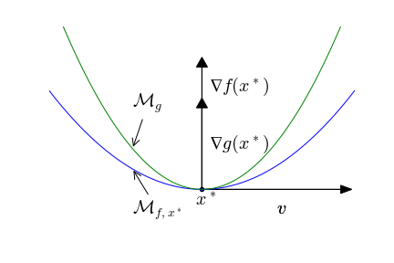
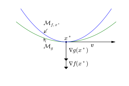
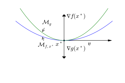
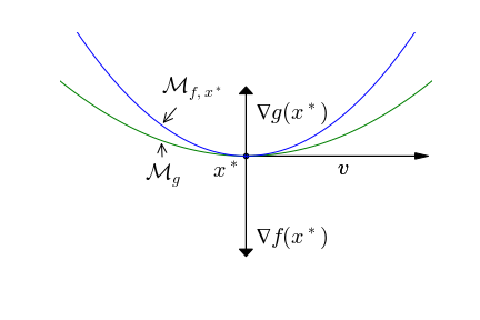
In an introductory course in optimization it makes sense to illustrate the first-order conditions (2) with a drawing, at least in the simple case $n=2$ and $m=1$ (curves on the plane): the two curves $\mathcal{M}_{f,x^{*}}$ and $\mathcal{M}_{g}$ in the plane $\mathbb{R}^{2}$ have a common tangent at point $x^{*}.$ Naturally follows the question for second-order conditions : how conditions (3) impose a new geometric contraint to first-order equation (2) ? How should the picture be in the simple case $n=2$ and $m=1$ ? Furthermore, since second-order conditions (3) with strict inequality combined with first-order conditions (2) also give sufficient conditions for $x^{*}\in\mathcal{M}_{g}$ to be a local minimum, it must garantee that $\mathcal{M}_{g}$ is locally on the half space $\mathcal{M}_{f,x^{*}}^{+}=\{x\in\mathbb{R}^{n}\,|\,f(x)\geq f(x^{*})\}.$

Let us start by considering the second-order conditions (3) in the case $n=2$ and $m=1:$

for every tangent vector $v\in\mathbb{R}^{2}$ of the curve $\mathcal{M}_{g}$ at point $x^{*}.$ We can take $v=v_{g}=(\partial_{x_{2}}g(x^{*}),-\partial_{x_{1}}g(x^{*}))^{T}$ or $v=v_{f}=(\partial_{x_{2}}f(x^{*}),-\partial_{x_{1}}f(x^{*}))^{T}=\lambda^{*}v_{g},$ since first-order conditions (2) are satisfied. We suppose that $\nabla f(x^{*})\neq 0,$ and consider the unit vectors $u_{g}=v_{g}/\|v_{g}\|$ and $u_{f}=v_{f}/\|v_{f}\|.$

A classical result of elementary differential geometry (see  [2]) gives the algebraic curvatures $\kappa_{f}(x^{*})$ and $\kappa_{g}(x^{*})$ of the curves $\mathcal{M}_{f,x^{*}}$ and $\mathcal{M}_{g}$ at a regular point $x^{*}$ :

Now, if we divide inequality (4) by $\|\nabla f(x^{*})\|$, take $v=u_{f}$ and use first-order conditions (2), we obtain

Therefore, the algebraic curvatures satisfy

with $+1$ if the vectors $\nabla f(x^{*})$ and $\nabla g(x^{*})$ have the same orientation and $-1$ otherwise. We can easily verify that inequality (6) on the curvatures is necessarily satisfied if $\mathcal{M}_{g}$ is locally on the half space $\mathcal{M}_{f,x^{*}}^{+}.$ Figure 1 gives, according to the sign of the algebraic curvatures, the four situations for which the curves $\mathcal{M}_{f,x^{*}}$ and $\mathcal{M}_{g}$ satisfy inequality (6).

To my knowledge, in the classical litterature on the subject, inequality (6) is not explicitly presented despite its intuitive and natural aspect.

In fact inequality (6) and more generally inequality (3) directly appears by requiring positivity of the second derivative of the function $(f\circ\gamma)(t)$ at $t=0$ (like for unconstrained minimization), for every regular curve $\gamma(t)$ in $\mathcal{M}_{g}$ such that $\gamma(0)=x^{*}$ (see  [3]).

By elementary calculus we obtain

In the particular case $m=1$, the constraint $\gamma(t)\in\mathcal{M}_{g},\,\forall t,$ gives

Combining inequality $(f\circ\gamma)^{\prime\prime}(0)\geq 0$ with (7), dividing by $\|\nabla f(x^{*})\|,$ and using first-order conditions (2), we obtain

which is equivalent to (6) in the particular case $n=2.$

The purpose of this note is to show how (8) can be seen, in the case $m=1$, as an inequality on the respective curvatures of the intersections of $\mathcal{M}_{f,x^{*}}$ and $\mathcal{M}_{g}$ with the affine plane $\mathcal{L}=\{x^{*}+a\gamma^{\prime}(0)+b\nabla f(x^{*}),\,\forall(a,b)\in\mathbb{R}^{2}\},$ and extend appropriately this property for any value of the codimension $m,\,1\leq m\leq n.$

The curvature of a manifold is a fundamental concept in differential geometry. It describes the way a curve or a surface deviates from being a straight line or a flat plane. A distinction exists between the notion of extrinsic curvature adapted for submanifolds embedded in an euclidean space and the notion of intrinsic curvature defined for Riemannian manifolds without reference to an ambiant euclidean space. As we deal with the submanifolds $\mathcal{M}_{f,x^{*}}$ and $\mathcal{M}_{g}$, we will consider the first notion of curvature.

In this paragraph we introduce the notion of second fundamental form and show its essential relation to the curvature (see  [6]) of a submanifold. Then, we determine the second fundamental forms of the submanifolds $\mathcal{M}_{f,x^{*}}$ and $\mathcal{M}_{g}$ at point $x^{*}.$ Finally we show how second-order necessary conditions (3) correspond to inequalities between the curvatures of the submanifolds $\mathcal{M}_{f,x^{*}}$ and $\mathcal{M}_{g}$ at point $x^{*}.$

We consider first the case of the hypersurface $\mathcal{M}_{f,x^{*}}=\{x\in\mathbb{R}^{n}\,|\,f(x)=f(x^{*})\}.$ We suppose that $x^{*}\in\mathbb{R}^{n}$ is a regular point of $f,$ i.e. $\nabla f(x^{*})\neq 0.$

Let $V\in\mathbb{R}^{n\times(n-1)}$ a matrix whose columns $v_{1},\cdots,v_{n-1}$ generate the tangent space $T_{x^{*}}\mathcal{M}_{f,x^{*}}.$ We define the function $\tilde{f}:\mathbb{R}^{n-1}\times\mathbb{R}\rightarrow\mathbb{R}$ by

for $a\in\mathbb{R}^{n-1}$ and $b\in\mathbb{R}.$ Since $\partial_{b}\tilde{f}(0,0)=\nabla f(x^{*})^{T}\nabla f(x^{*})\neq 0,$ by using the implicit function theorem, we can define an open ball $B(0,r)\subset\mathbb{R}^{n-1}$ of radius $r>0,$ a centered open interval $I_{r^{\prime}}=]-r^{\prime},r^{\prime}[\subset\mathbb{R}$ (with $r^{\prime}>0$), and an implicit function $\varphi:B(0,r)\rightarrow I_{r^{\prime}}$ such that

The implicit function $\varphi$ satisfies $\varphi(0)=0,$ and $\nabla\varphi(0)=0.$ The first equality is due to the unicity of the implicit function. The second is deduced from the equality $\nabla\varphi(0)^{T}=-(\nabla f(x^{*})^{T}\nabla f(x^{*}))^{-1}\,\nabla f(x^{*})^{T}V,$ satisfied by the gradient of the implicit function $\varphi$ and $\nabla f(x^{*})^{T}V=0,$ since the columns of $V$ are vectors of $T_{x^{*}}\mathcal{M}_{f,x^{*}}.$

The restriction of the implicit function $\varphi$ to a line $\mathbb{R}v$ generated by a fixed tangent vector $v\in T_{x^{*}}\mathcal{M}_{f,x^{*}}$ defines an implicit curve of $\mathcal{M}_{f,x^{*}}.$ More precisely, if $v=Va$ for some $a\in\mathbb{R}^{n-1},\,a\neq 0,$ we can define the function $\varphi_{a}(t)=\varphi(ta)$ for all $t\in\mathbb{R}$ such that $ta\in B(0,r).$ Let $\mathcal{L}_{f,v}$ the normal section defined by the tangent vector $v,$ $\mathcal{L}_{f,v}=\{x^{*}+tv+b\nabla f(x^{*}),\,\forall(t,b)\in\mathbb{R}\times\mathbb{R}\}.$ The curve $\gamma(t)=x^{*}+tv+\varphi_{a}(t)\nabla f(x^{*})$ defined for all $t\in\mathbb{R}$ such that $ta\in B(0,r)$ lies in the intersection $\mathcal{M}_{f,x^{*}}\cap\mathcal{L}_{f,v}$ and satisfies $\gamma(0)=x^{*}$ and $\gamma^{\prime}(0)=v$ since $\varphi_{a}(0)=0$ and $\varphi^{\prime}_{a}(0)=0.$ By taking $v\in T_{x^{*}}\mathcal{M}_{f,x^{*}},\,\|v\|=1,$ and re-parametrizing the curve $\gamma$ by arc length, we get a curve satifying the hypotheses of proposition 2.

For the submanifold $\mathcal{M}_{g}$ the results are obtained in the same way.

Let $V\in\mathbb{R}^{n\times(n-m)}$ a matrix whose columns $v_{1},\cdots,v_{n-m}$ generate the tangent space $T_{x^{*}}\mathcal{M}_{g}.$ We define the function $\tilde{g}:\mathbb{R}^{n-m}\times\mathbb{R}^{m}\rightarrow\mathbb{R}^{m}$ by

for $a\in\mathbb{R}^{n-m}$ and $b\in\mathbb{R}^{m}.$ The Jacobian matrix $J_{b}\tilde{g}(0,0)$ of the function $\tilde{g}$ relatively to the variable $b$ is given by

and thus, since $Jg(x^{*})$ is full rank, $J_{b}\tilde{g}(0,0)$ is invertible. We can apply again the implicit function theorem : there exist an open ball $B(0,\overline{r})\subset\mathbb{R}^{n-m}$ of radius $\overline{r}>0,$ an open ball $B(0,\overline{r}^{\prime})\subset\mathbb{R}^{m}$ of radius $\overline{r}^{\prime}>0,$ and an implicit function $\psi:B(0,\overline{r})\rightarrow B(0,\overline{r}^{\prime})$ such that

Again, the implicit function $\psi$ verifies $\psi(0)=0,$ and $J\psi(0)=0.$

Finally, the restriction of the implicit function $\psi$ to a line $\mathbb{R}v$ generated by a fixed vector $v\in T_{x^{*}}\mathcal{M}_{g}$ defines an implicit curve in the intersection $\mathcal{M}_{g}\cap\mathcal{L}_{g,v},$ where $\mathcal{L}_{g,v}$ is the affine subspace $\mathcal{L}_{g,v}=\{x^{*}+tv+Jg(x^{*})^{T}b,\,\forall(t,b)\in\mathbb{R}\times\mathbb{R}^{m}\}.$

In order to show the sufficient second-order sufficient conditions, we consider the function $F:B(0,\overline{r})\rightarrow\mathbb{R},$ defined by

where as above, the implicit function $\psi:B(0,\overline{r})\rightarrow B(0,\overline{r}^{\prime}),$ with $B(0,\overline{r})\subset\mathbb{R}^{n-m}$ and $B(0,\overline{r}^{\prime})\subset\mathbb{R}^{m},$ verifies

Using the properties of $\psi$, we get $\nabla F(0)^{T}=\nabla f(x^{*})^{T}V.$ But, from first-order optimality conditions, we have $T_{x^{*}}\mathcal{M}_{g}\subset T_{x^{*}}\mathcal{M}_{f,x^{*}},$ and thus $\nabla F(0)=0,$ since the columns of $V$ are vectors of the tangent space $T_{x^{*}}\mathcal{M}_{g}.$

By derivating twice we get the Hessian matrix $\nabla^{2}F(0)$ :

where $\nabla^{2}\psi_{j}$ is the Hessian matrix of the $j$th component of the implicit function $\psi$ ($\psi=(\psi_{1},\cdots,\psi_{m})$).

In the same way, by derivating equation (15) twice, we get, for $a=0$,

The Hessian matrix $\nabla^{2}F(0)$ is related to the Hessian matrix $\nabla_{xx}^{2}L(x^{*},\lambda^{*}).$

References

- [1] Do Carmo, M. (1992). Riemannian Geometry. Birkhaüser.
- [2] Goldman, R. (2005). Curvature formulas for implicit curves and surfaces. Comput. Aided Geom. Des., 22, 632-658.
- [3] Luenberger, D. G., Ye, Y.(2008). Linear and Nonlinear Programming. 4th ed. Springer.
- [4] Nocedal, J., Wright, S. J. (2006). Numerical Optimization. 2nd ed. Springer.
- [5] Rapcsák, R. (1997). Smooth Nonlinear Optimization in . Springer Science + Business Media.
- [6] Robbin, J. W., Salamon, D. A. (2022). Introduction to Differential Geometry. Springer.
- [7] Thorpe, J. A. (1979). Elementary Topics in Differential Geometry. Springer-Verlag.