Covariance–based rational approximations of fractional SPDEs for computationally efficient Bayesian inference

Handling many observations from a Gaussian random field in spatial statistics can be challenging since the related computational tasks involve factorizations of large covariance matrices which are usually dense. This is often referred to as the “big $N$ problem” (Banerjee et al. 2015), and various approaches have been suggested to handle the computational issues (see, e.g., Heaton et al. 2019, for a recent comparison). One of the most widely used methods is the SPDE approach by Lindgren et al. 2011. This is based on the fact that a centered Gaussian random field $u$ on the spatial domain $\mathcal{D}=\mathbb{R}^{d}$ with an isotropic Matérn covariance function (Matérn 1960),

can be represented as a solution to the stochastic partial differential equation (SPDE)

Here, $\Gamma(\cdot)$ is the Gamma function, $K_{\nu}$ is a modified Bessel function of the second kind, $\Delta$ is the Laplace operator, and $\mathcal{W}$ is Gaussian white noise. The parameter $\kappa>0$ controls the practical correlation range, $\sigma^{2}$ is the variance, $\tau^{2}=\Gamma(\nu)/(\sigma^{2}\kappa^{2\nu}(4\pi)^{d/2}\Gamma(\nu+d/2))$, and the fractional power $\beta$ is related to the smoothness parameter $\nu>0$ via the relation $2\beta=\nu+d/2$ (Whittle 1963). Lindgren et al. 2011 used this representation to construct computationally efficient Gaussian Markov Random Field (GMRF) approximations of Gaussian Matérn fields by considering the SPDE on a bounded domain $\mathcal{D}$, restricting the smoothness to $2\beta\in\mathbb{N}$, and then performing a finite element method (FEM) discretization.

The SPDE approach has become widely used in applications, and has initiated a great number of extensions and generalizations (Lindgren et al. 2022). The reason for this is not only the computational benefits, but also that it provides a flexible framework for defining more sophisticated models for spatial data. It, for example, facilitates the construction of non-stationary Gaussian random fields by allowing the parameters $\kappa$ and $\tau$ to be spatially varying (Lindgren et al. 2011; Fuglstad et al. 2015), and allows for the construction of Matérn-like random fields on more general manifolds by defining such fields via the SPDE (2) posed on the manifold (Lindgren et al. 2011; Bolin and Lindgren 2011).

One of the main criticisms of the SPDE approach is the requirement $2\beta\in\mathbbm{N}$, which restricts the possible values of the corresponding smoothness parameter $\nu$ of the Matérn covariance function. Given the importance of $\nu$ when performing prediction, as shown by Stein 1999 and Bolin and Kirchner 2023, several methods for removing the restriction of $2\beta\in\mathbbm{N}$ have been proposed. Lindgren et al. 2011 proposed to construct a GMRF approximation by approximating the spectrum of a Gaussian Matérn field by a spectrum that is a reciprocal of a polynomial. This method is applicable for stationary models but it can not be applied to non-stationary models, and it has a fixed accuracy which may not be sufficient for certain applications. Bolin et al. 2020 proposed combining the FEM approximation of Lindgren et al. 2011 with a quadrature approximation of the fractional operator to obtain a numerical method that works for any $\beta>d/4$ and can be made arbitrarily accurate. That work also provided a theoretical convergence analysis of the method, which was extended in Bolin et al. 2018 and Herrmann et al. 2020. Bolin and Kirchner 2020 later proposed a different type of approximation referred to as the rational SPDE approach, which has a lower computational cost.

Even though the methods that work for non-stationary models with general smoothness are computationally efficient, they are much less used than the standard SPDE approach for statistical applications. The reason for this is that non-fractional SPDE models work in combination with the integrated nested Laplace approximation (INLA) method (Rue et al. 2009) and are implemented in the widely used R-INLA (Lindgren and Rue 2015) R (R Core Team 2022) package. This software facilitates including SPDE-based models in general Bayesian latent Gaussian models, and the great majority of all applications of the SPDE approach have been done via this software.

Unfortunately, the methods of Bolin et al. 2020 and Bolin and Kirchner 2020 provide approximations which are not compatible with R-INLA. The reason is that the methods do not yield a Markov approximation, so the precision matrix obtained from the approximations are not sparse. The covariance matrix of the approximations are of the form $\mathbf{P}\mathbf{Q}^{-1}\mathbf{P}$, where both $\mathbf{P}$ and $\mathbf{Q}$ are sparse matrices that depend on the parameters of the model. To achieve a sparse precision matrix, which is necessary for R-INLA, Bolin and Kirchner 2020 showed that one can work with a latent model with sparse precision matrix $\mathbf{Q}$ if the projection matrix $\mathbf{A}$, which connects the locations of the mesh for the FEM approximation and the observation locations (see Section 2 for details), is adjusted to $\widehat{\mathbf{A}}=\mathbf{A}\mathbf{P}$. This matrix, however, depends on the model parameters, which is not allowed in R-INLA.

The main goal of this work is to solve this problem by proposing an alternative rational approximation. The main idea is to approximate the covariance operator of the random field directly, instead of first approximating the solution $u$ and then deriving the corresponding covariance operator. This provides an approximation suitable for R-INLA, which is more numerically stable than that of the original rational SPDE approach. The proposed method is implemented in the R package rSPDE (Bolin and Simas 2023), which is available on CRAN and has an interface to R-INLA. Using the package, we show that the proposed method facilitates full Bayesian inference of all model parameters, including $\beta$, for latent Gaussian models based on fractional SPDEs.

The outline of the paper is as follows. In Section 2, we give an overview of the model structure of the proposed approximation and show how it can be used for computationally efficient inference. The mathematical details and justifications of the method are provided in Sections 3 to 5. Specifically, in Section 3, we introduce the generalized Whittle–Matérn fields, which contain most of the previously proposed non-stationary SPDE-based Gaussian random fields as special cases, and for which our proposed method is applicable. In that section, we also provide the details of the FEM approximations. The new covariance-based rational approximation is introduced in Section 4, where we also prove that it provides an approximation of the covariance function of the generalized Whittle–Matérn field with an explicit rate of convergence in the $L_{2}$-norm. In Section 5, we show that the covariance-based rational approximation can be represented as a GMRF, and illustrate how this can be used for statistical inference. Some of the details of the rSPDE implementation are discussed in Section 6, and a comparison in terms of the accuracy of approximating covariance function by our method and some other methods is provided in Section 7. An application to modeling of precipitation data is presented in Section 8 and the article concludes with a discussion in Section 9. Finally, the supplementary materials contain seven appendices which provide further technical details and proofs.

As mentioned in the introduction, the main idea behind our strategy is to directly approximate the covariance operator of the random field. In this section we show the structure of the resulting approximation and also provide an illustration on how it can be used for inference in a simple application. More details will be given in later sections. The covariance-based rational approximation of the Whittle–Matérn field $u(\boldsymbol{s})$ defined in (2), whose covariance operator is $(\kappa^{2}-\Delta)^{-2\beta}$, uses a combination of the finite element method and rational approximations in order to approximate $u(\boldsymbol{s})$ as $u_{n}(\boldsymbol{s})=\sum_{j=1}^{n}w_{j}\varphi_{j}(\boldsymbol{s})$, where $\{w_{j}\}_{j=1}^{n}$ are stochastic weights and $\{\varphi_{j}\}_{j=1}^{n}$ are FEM basis functions. We denote $\boldsymbol{w}=[w_{1},...,w_{n}]^{\top}$. With our approximation, $\boldsymbol{w}$ can be expressed as a sum of $m+1$ independent GMRFs with sparse precision matrices:

Any linear predictor in R-INLA has this form, which means that we can perform inference in a computationally efficient manner based on the covariance-based rational approximation by using the same ideas as are used in R-INLA. For example, suppose that we observe $y_{1},\ldots,y_{N}$, $N\in\mathbb{N}$, where

$\boldsymbol{s}_{1},\ldots,\boldsymbol{s}_{N}\in\mathbb{R}^{d}$ are spatial locations, and $\boldsymbol{\epsilon}=[\epsilon_{1},...,\epsilon_{N}]^{\top}\sim N(\textbf{0},\boldsymbol{Q}^{-1}_{\boldsymbol{\epsilon}})$ for some sparse matrix $\boldsymbol{Q}_{\boldsymbol{\epsilon}}$, such as $\boldsymbol{Q}_{\boldsymbol{\epsilon}}=\frac{1}{\sigma_{\epsilon}^{2}}\boldsymbol{I}_{N}$ if we have independent measurement noise. Defining $\boldsymbol{y}=[y_{1},...,y_{N}]^{\top}$, (4) can be written in matrix form as $\boldsymbol{y}=\textbf{A}\boldsymbol{w}+\boldsymbol{\epsilon}$, where A is the projector matrix with elements $A_{ij}=\varphi_{j}(\boldsymbol{s}_{i})$. Let $\boldsymbol{X}=[\boldsymbol{x}^{\top}_{1},...,\boldsymbol{x}^{\top}_{m+1}]^{\top}$. Then, the precision matrix of $\boldsymbol{X}$ is the block diagonal matrix

Writing the model in terms of the weights $\boldsymbol{X}$ allows us to equivalently write the model as $\boldsymbol{y}=\overline{\boldsymbol{A}}\boldsymbol{X}+\boldsymbol{\epsilon}$ where $\overline{\boldsymbol{A}}$ is a block matrix of size $N\times n(m+1)$ obtained by combining $m+1$ copies of $\boldsymbol{A}$ as $\overline{\boldsymbol{A}}=\begin{bmatrix}\boldsymbol{A}&\cdots&\boldsymbol{A}\end{bmatrix}$. Thus, $\boldsymbol{y}|\boldsymbol{X}\sim N(\overline{\boldsymbol{A}}\boldsymbol{X},\boldsymbol{Q}^{-1}_{\boldsymbol{\epsilon}})$ and $\boldsymbol{X}\sim N(\textbf{0},\boldsymbol{Q}^{-1})$, where $\boldsymbol{Q}$ is given in (5). Standard results for latent Gaussian models then give us that the posterior distribution of $\boldsymbol{X}$ is $\boldsymbol{X}|\boldsymbol{y}\sim N(\boldsymbol{\mu}_{\boldsymbol{X}|\boldsymbol{y}},\boldsymbol{Q}^{-1}_{\boldsymbol{X}|\boldsymbol{y}})$, where

Finally, we can obtain the marginal likelihood, $\ell(\boldsymbol{y})$, of $\boldsymbol{y}$ as

The sparsity of $\boldsymbol{Q}$ is essential for computation. For instance, evaluating $\log|\boldsymbol{Q}|$ in the likelihood can be done efficiently based on sparse Cholesky decomposition (Rue and Held 2005). Sparsity of $\boldsymbol{Q}$ also facilitates computationally efficient sampling of $\boldsymbol{w}$, and hence of $u$. See Appendix E for further details on the methods for sampling and likelihood evaluation.

In this section we introduce the class of fractional-order SPDEs we are interested in as well as their FEM approximations. The model assumptions are presented in Section 3.1, and in Section 3.2 we introduce the FEM approximations and study their convergence.

Let us begin by introducing some notation that will be needed later on. Given a bounded domain $\mathcal{D}\subset\mathbb{R}^{d}$, $d\in\{1,2,3\}$, we denote by $L_{2}(\mathcal{D})$ the Lebesgue space of square-integrable real-valued functions endowed with the inner product ${(\phi,\psi)_{L_{2}(\mathcal{D})}=\int_{\mathcal{D}}\phi(\boldsymbol{x})\psi(\boldsymbol{x})d\boldsymbol{x}}$. We denote the Sobolev space of order $k$ by $H^{k}(\mathcal{D})$:

where we are using the multiindex notation for the differential operator $D^{\gamma}$, and $(\cdot,\cdot)_{H^{k}(\mathcal{D})}$ is the Sobolev inner product:

We denote by $H_{0}^{1}(\mathcal{D})$ the closure of $C_{c}^{\infty}(\mathcal{D})$ in $H^{1}(\mathcal{D})$, where $C_{c}^{\infty}(\mathcal{D})$ is the set of infinitely differentiable functions with compact support on $\mathcal{D}$. Additional notations needed for the theoretical analysis are given in Appendix A.

Having introduced the FEM approximation, we are now ready to define the complete approximation of the covariance operator of the generalized Whittle–Matérn fields. The approximation is obtained by combining a rational approximation of the fractional power of the covariance operator with the FEM approximation. We begin by introducing the method and then provide a theoretical justification by showing an explicit rate of convergence of the approximate covariance function to the correct one in the $L_{2}(\mathcal{D}\times\mathcal{D})$-norm.

In Bolin and Kirchner 2020, the authors obtained an approximation of the solution to (8), which also implicitly defines an approximation of the corresponding covariance operator. However, as we have previously mentioned, this results in an approximation that is not implementable in R-INLA. Also, for statistical applications there is usually no need to have an approximation of the solution itself, since only the corresponding distribution matters for inference. With this in mind, we propose to directly approximate the covariance operator $L^{-2\beta}$. To this end, we first split $L_{h}^{-2\beta}=L_{h}^{-\{2\beta\}}L_{h}^{-\lfloor 2\beta\rfloor}$, where $\{x\}=x-\lfloor x\rfloor$ is the fractional part of $x$. Then, we approximate $L_{h}^{-\{2\beta\}}$ with a rational approximation. This yields an approximation

Here, $p(L_{h}^{-1})=\sum_{i=0}^{m}a_{i}L_{h}^{m-i}$ and $q(L_{h}^{-1})=\sum_{j=0}^{m}b_{j}L_{h}^{m-j}$ are polynomials obtained from a rational approximation of order $m$ of the real-valued function $f(x)=x^{\{2\beta\}}$. That is,

Specifically, to obtain $\{a_{i}\}_{i=0}^{m}$ and $\{b_{i}\}_{i=0}^{m}$, we approximate the function $f(x)=x^{\{2\beta\}}$ on the interval $[\lambda_{n_{h},h}^{-1},\lambda_{1,h}^{-1}]$, which covers the spectrum of $L^{-1}_{h}$. The coefficients are computed as the best rational approximation in the $L_{\infty}$-norm, which, for example, can be obtained via the second Remez algorithm (Remez 1934) or by the recent, and more stable, BRASIL algorithm (Hofreither 2021). See Appendix F for details about this algorithm and a justification for the choice of using the best rational approximation in $L_{\infty}$-norm.

By defining the covariance function

we have that $\varrho_{h,m}^{\beta}$ is the kernel of the covariance operator $L_{h,m}^{-2\beta}$. There are two sources of errors when we consider $\varrho_{h,m}^{\beta}$ as an approximation of the true covariance function $\varrho^{\beta}$ of the generalized Whittle–Matérn field: the FEM approximation and the rational approximation. The following proposition, whose proof is given in Appendix B, shows that we have control of these two sources of errors via the FEM mesh width $h$ and the order of the rational approximation $m$.

The goal of this section is to obtain a sparse matrix representation of the precision operator of the rational approximation from the previous section, so that the methods in Section 2 can be used for computationally efficient sampling and likelihood evaluation.

The solution $u_{h}$ in (10) at spatial location $\boldsymbol{s}$ can be represented as $u_{h}(\boldsymbol{s})=\sum_{j=1}^{n_{h}}w_{j}\varphi_{j}(\boldsymbol{s})$, where $\{w_{j}\}_{j=1}^{n_{h}}$ are stochastic weights and $\{\varphi_{j}\}_{j=1}^{n_{h}}$ are the piecewise linear finite element basis functions. We will now show how to represent $\boldsymbol{w}=[w_{1},...,w_{n_{h}}]^{\top}$ as a sum of independent GMRFs, each with a sparse precision matrix. The key step is to apply a partial fraction decomposition in (12):

Here, $\{r_{i}\}_{i=1}^{m}$, $\{p_{i}\}_{i=1}^{m}$ and $k$ are real numbers, and $I_{V_{h}}$ is the identity operator mapping the finite element space to itself. Let $\boldsymbol{C}$ be the mass matrix with elements $\boldsymbol{C}_{i,j}=(\varphi_{i},\varphi_{j})_{L_{2}(\mathcal{D})}$, and let $\boldsymbol{L}$ be the matrix obtained by the bilinear form $a_{L}(\cdot,\cdot)$ induced by the differential operator $L$, which has elements ${\boldsymbol{L}_{i,j}=(\boldsymbol{H}\nabla\varphi_{i},\nabla\varphi_{j})_{L_{2}(\mathcal{D})}+(\kappa^{2}\varphi_{i},\varphi_{j})_{L_{2}(\mathcal{D})}}$. Then, we can use (14) to obtain the covariance matrix of $\boldsymbol{w}$ as (see Appendix C for a derivation):

where $\boldsymbol{K}_{0}=k\boldsymbol{C}$ and $\boldsymbol{K}_{n}=k(\boldsymbol{L}^{-1}\boldsymbol{C})^{n-1}\boldsymbol{L}^{-1}$ when $n\geq 1,n\in\mathbb{N}$. In the Matérn case, that is, when $\kappa$ is a constant and $\boldsymbol{H}$ is an identity matrix, we simply have ${\boldsymbol{L}=\boldsymbol{G}+\kappa^{2}\boldsymbol{C}}$, where $\boldsymbol{G}$ is the stiffness matrix with elements $\boldsymbol{G}_{i,j}=(\nabla\varphi_{i},\nabla\varphi_{j})_{L_{2}(\mathcal{D})}$.

Since we have the same degree for numerator and denominator in the rational approximation, we can use the BRASIL algorithm (Hofreither 2021) to compute the coefficients $\{a_{i}\}_{i=0}^{m}$ and $\{b_{i}\}_{i=0}^{m}$ in (12) and thus the coefficients $\{r_{i}\}_{i=0}^{m}$, $\{p_{i}\}_{i=0}^{m}$ and $k$ in (14). Another option, commonly used in practice, is to use a “near best” rational approximation. One such option, which was used in Bolin and Kirchner 2020, and which is also implemented in the rSPDE package, is the Clenshaw–Lord Chebyshev–Padé algorithm (Baker and Graves-Morris 1996). See Appendix F for details about this algorithm. Also, observe that the interval $[\lambda_{n_{h},h}^{-1},\lambda_{1,h}^{-1}]$ where one should compute the rational approximation may vary with the parameters $\kappa$ and $\boldsymbol{H}$, and that recomputing the coefficients $\{a_{i}\}_{i=0}^{m}$ and $\{b_{i}\}_{i=0}^{m}$ for different values of these parameters is not practical for implementations. To avoid this, recall from Assumption 2 that $\kappa_{0}^{2}$ is a lower bound for the eigenvalues of $L$ in the case of Neumann boundary conditions and that $\lambda_{1}\leq\lambda_{1,h}$ (see Proposition 3 in Appendix B). We can, then, re-scale the operator $L_{h}$ as $L_{h}/\kappa_{0}^{2}$ so that we can replace the interval $[\lambda_{n_{h},h}^{-1},\lambda_{1,h}^{-1}]$ by $[\delta,1]$, where, ideally, $\delta$ is chosen in such way that $\delta\leq\kappa_{0}^{2}/\lambda_{n_{h},h}$ for all considered mesh sizes $h$. In the rSPDE package, the choices $\delta=0$ and $\delta=10^{-(5+m)/2}$ are implemented. However, the difference in accuracy with respect to approximating the covariance function is negligible between these two choices.

For these options, we verified empirically that if $f_{\beta}(x)=x^{\{2\beta\}}$, $\{2\beta\}=2\beta-\lfloor 2\beta\rfloor$, and $\widehat{f}_{\beta,m}$ is the rational approximation of $f_{\beta}$ where the numerator and denominator have same degree $m$, then $\widehat{f}_{\beta,m}=x^{\lfloor 2\beta\rfloor}\sum_{j=1}^{m}r_{i}(x-p_{i})^{-1}+k,$ where $\{p_{i}\}_{i=1}^{m}$ are negative real numbers and $\{r_{i}\}_{i=1}^{m}$ and $k$ are positive real numbers. This, together with the fact that the BRASIL algorithm is only implemented for rational approximations with numerator and denominator having the same degree, are the main reasons we chose to consider the numerator and denominator having the same degree $m$. Bolin and Kirchner 2020 instead considered a rational approximation where the numerator has degree $m$ and the denominator has degree $m+1$. However, with this choice the partial fractions would not yield a decomposition into positive-definite operators in our case.

Since $\{p_{i}\}_{i=1}^{m}$ are negative real numbers and $\{r_{i}\}_{i=1}^{m}$ and $k$ are positive real numbers, we have that $r_{i}(\boldsymbol{L}^{-1}\boldsymbol{C})^{\lfloor 2\beta\rfloor}(\boldsymbol{L}-p_{i}\boldsymbol{C})^{-1}$, for $i=1,...m$, and $\boldsymbol{K}_{\lfloor 2\beta\rfloor}$ are valid covariance matrices. Thus, $\boldsymbol{w}$ can be expressed as a sum of $m+1$ independent random vectors $\boldsymbol{x}_{i}$ as in (3), where $\boldsymbol{Q}_{i}$ is the precision matrix of $\boldsymbol{x}_{i}$. By (15), we obtain that

Let $\boldsymbol{X}=[\boldsymbol{x}^{\top}_{1},...,\boldsymbol{x}^{\top}_{m+1}]^{\top}$. Then, the precision matrix of $\boldsymbol{X}$ is the block diagonal matrix shown in (5). The final step in order to obtain a GMRF representation is to use the mass lumping technique as for the standard SPDE approach, see Appendix C.5 in Lindgren et al. 2011. Thus, the mass matrix $\boldsymbol{C}$ in (16) is replaced by a lumped mass matrix $\tilde{\boldsymbol{C}}$, where $\tilde{\boldsymbol{C}}$ is a diagonal matrix with $\tilde{\boldsymbol{C}}_{ii}=\sum_{j=1}^{n_{h}}\boldsymbol{C}_{ij}$, for $i=1,...,n_{h}$. With this adjustment, $\boldsymbol{Q}$ in (5) is sparse and we thus have obtained a GMRF representation.

The proposed covariance-based rational approximation method has been implemented in the R package rSPDE. In the following sections, we will use this package to illustrate the performance of the method. In this section, we give a brief introduction to the package and how it can be used in combination with R-INLA for computationally efficient Bayesian inference of latent Gaussian models involving the generalized Whittle–Matérn fields.

The usual workflow of fitting standard SPDE models in R-INLA can be divided into six steps. Namely, constructing the FEM mesh, defining SPDE model, creating a projector matrix, building the INLA stack, specifying the model formula, and finally calling the function inla to fit the model. Details about this can be found in Lindgren and Rue 2015. To fit a model with a fractional SPDE, this procedure remains the same. The only difference is that when defining the SPDE model, creating the projector matrix and building the index for INLA stack, we use functions from the rSPDE package. These functions are very similar to the corresponding R-INLA functions in terms of functionality. For example, a fractional SPDE model can be created with the command:

Ψmodel <- rspde.matern(mesh = mesh)

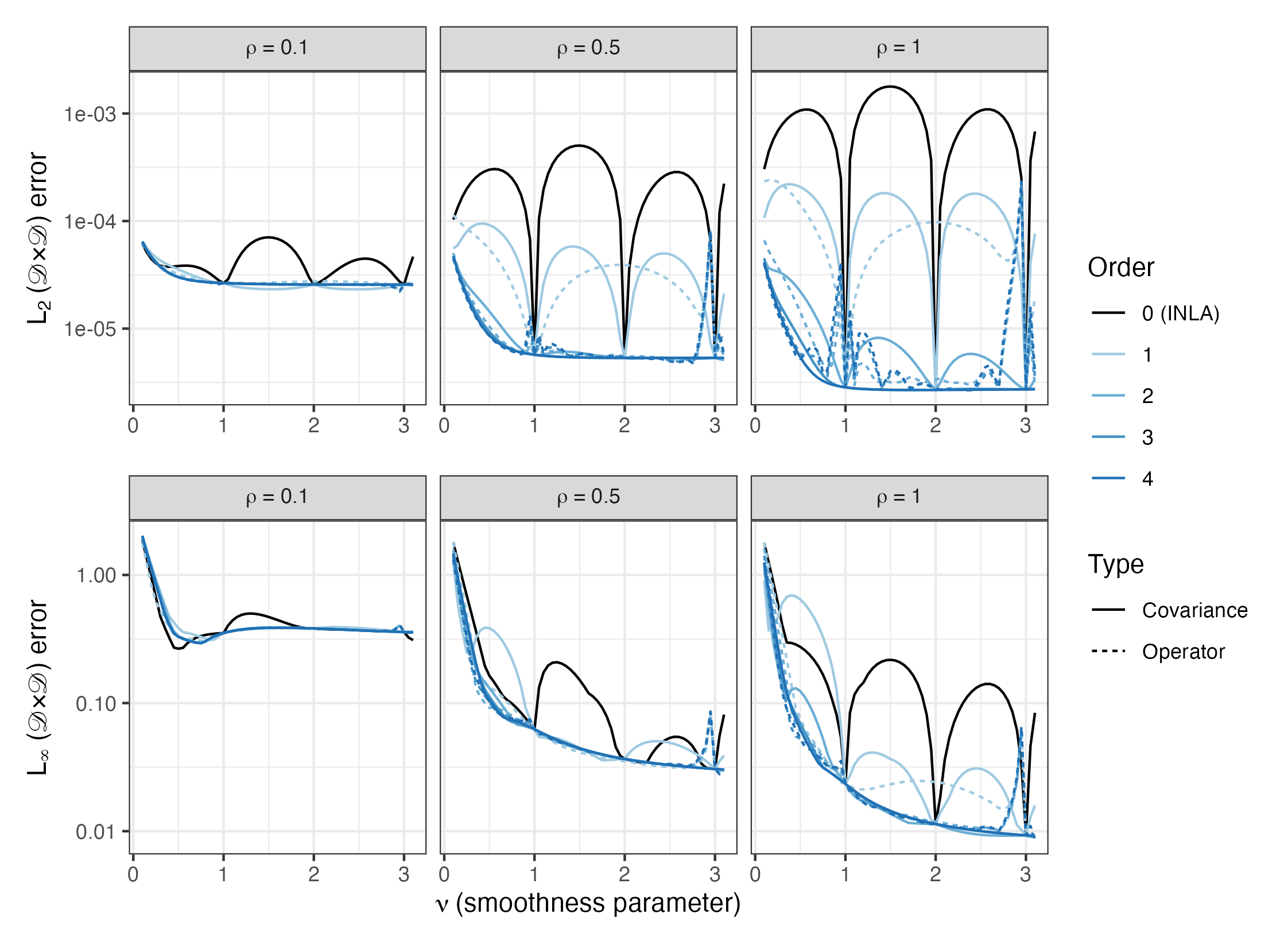
where mesh is a FEM mesh that can be obtained by inla.mesh.2d function from R-INLA. The default order of the rational approximation in this function is $m=2$, which provides a good trade off between computational cost and accuracy, see Figures 1 and 6. As for the corresponding inla.spde2.matern function that can be used to define non-fractional SPDE models in INLA, one can also set priors for $\kappa$ and $\tau$ in rspde.matern. Further, we can also define a prior for the smoothness parameter $\nu$ or specify $\nu$ so that a SPDE model with a fixed smoothness parameter can be generated. This feature can be used, for example, in the case that one already knows what $\nu$ is or wants to compare two different models with different $\nu$, as we will do in Section 8.

The projector matrix $\overline{\boldsymbol{A}}$ for a given mesh and observation locations loc is computed as

ΨA <- rspde.make.A(mesh = mesh, loc = loc)

As for the creation of the model, the default order of the rational approximation when creating the projector matrix is $m=2$, which can be changed by the user. The other arguments of the function are the same as those in the corresponding R-INLA function inla.spde.make.A. In the step of building the INLA stack, usually an index set is needed. The index can be computed with the function rspde.make.index, which replaces the R-INLA function inla.spde.make.index and has the same arguments. With these functions, the fractional models can be used as any other random effect in R-INLA. After fitting the model with the R-INLA function inla, posterior samples from a latent field and hyperparameters can be obtained by using inla.posterior.sample, and posterior distributions of the model parameters can be extracted via the rSPDE function rspde.result.

Besides the INLA-related functions, the rSPDE package also provides various utility functions. For example, once a fractional SPDE model, model, has been created with the rspde.matern function, one can simulate from it by calling simulate(model) to obtain a prior sample from a given choice of parameters, and the marginal log-likelihood from Section 2 can be computed by

Ψl <- rSPDE.matern.loglike(model, y, A, sigma.e)

Here, y is the observed data and sigma.e is the standard deviation of the measurement noise. In addition, if a model is fitted with this approach, then kriging and posterior sampling can be obtained by using the predict function. For further details and examples, we refer the reader to the vignettes at https://davidbolin.github.io/rSPDE.

Finally, rSPDE also provides an interface to the inlabru package (Bachl et al. 2019), which simplifies the construction of spatial models. This was used in the application in Section 8, where the entire code for defining and fitting the fractional model is:

Ψmesh <- inla.mesh.2d(loc = loc, max.edge = c(0.5, 10), cutoff = 0.35)
Ψspde <- rspde.matern(mesh = mesh, nu.upper.bound = 1)
Ψres <- bru(z ~ -1 + field(coordinates, model = spde), data = data)

Here loc are the measurement locations and data is a data frame with the locations and observations.

In this section, we compare the accuracy of the covariance–based rational approximation with the operator-based method from Bolin and Kirchner 2020, and with the “parsimonious” method from Lindgren et al. 2011. Since the latter method is implemented in R-INLA, we refer to it as the INLA approximation. We also note that the INLA method constructs a covariance-based Markov approximation (see also Bolin and Kirchner 2020, Section 2), so it can be viewed as a $0$th order covariance-based rational approximation.

For the comparison, we consider the SPDE model (2) with homogeneous zero Neumann boundary conditions on the unit square $\mathcal{D}=[0,1]^{2}$, with $\tau$ chosen such that $\sigma^{2}$ in the Matérn covariance is one. The reason we consider the square domain, is that we have an explicit expression for the covariance function of the solution $u$. Indeed, we have, from Khristenko et al. 2019, that the covariance function of $u$ is given by

where $\|\cdot\|$ is the Euclidean norm on $\mathbb{R}^{2}$ and $\varrho(\cdot)$ is the Matérn covariance function in (1) with $\sigma=1$ and $\nu=2\beta-1$. To compare the accuracy of the covariance approximations, we evaluate the true and approximate covariance functions on a regular mesh on $[0,1]^{2}$ with $N=100$ equally spaced nodes on each axis. We will compare these approximations with respect to the ${L_{2}([0,1]^{2}\times[0,1]^{2})}$-norm and the supremum norm on $[0,1]^{2}\times[0,1]^{2}$. Appendix G shows how we approximate the errors in these two norms in detail.

For the operator-based and covariance-based rational approximations, we consider the orders of rational approximation as $m=1,2,3,4$. We choose smoothness parameters ranging from $0.1$ to $3.1$ with steps of size $0.05$. Further, we test three possible values of $\kappa$. These values of $\kappa$, say $\kappa_{1}(\nu),\kappa_{2}(\nu)$ and $\kappa_{3}(\nu)$ are chosen in such a way that the practical range $\rho=\sqrt{8\nu}/\kappa$ is fixed as $0.1,0.5$ and $1$, respectively, for all values of $\nu$. The resulting errors for the different methods are shown in Figure 1.

We begin by observing that for smoothness parameters $\nu=1,2$ or $3$, there is no rational approximation and the errors only come from the FEM approximation. With this in mind, one should note that for smaller range parameters most of the approximation error comes from the FEM approximation, thus yielding a small difference of errors across the different methods. However, for larger ranges, such as, in this case, practical range equal to $1$, the errors have different orders of magnitude as the order of the rational approximation increases, with the errors from the operator-based and covariance-based approximations of same rational approximation order having approximately the same order of magnitude. Furthermore, we can observe numerical instabilities of the operator-based approximations of order 3 and 4 as $\nu$ increases for both practical ranges $0.5$ and $1$, whereas the covariance-based method is stable for all orders of approximation.

In order to further illustrate the effect of the FEM error on the rational approximation of the covariance operator we repeated the analysis from above but with a coarser FEM mesh, consisting of 50 equally spaced nodes on each axis over the domain $[0,1]^{2}$. The results are shown in Figure 6 in Appendix G. We now observe that for practical range $0.1$, there is no visible difference between the covariance-based or operator-based rational approximations of orders 1 to 4, with a very small difference between the “parsimonious” INLA approximation and the remaining rational approximations. Further, for practical ranges $0.5$ and $1$, we hardly see any differences between the rational approximations of orders $2$, $3$ and $4$. The only noticeable difference being that for large values of $\nu$, the operator-based rational approximation becomes numerically unstable. On the other hand, it is noteworthy that for practical ranges $0.5$ and $1$, there is a significant difference (difference in orders of magnitude) between the rational approximations of order 0, 1 and the remaining orders.

To summarize, the results indicate that the covariance-based method generally has a similar accuracy as the operator-based method, which is higher than the accuracy provided by INLA’s method. The results also show that the covariance-based method is more numerically stable, especially for larger values of $m$, the order of the rational approximation.

It is important to remember that the INLA method only provides a fixed approximation, furthermore it only works in this case of stationary parameters, whereas the other methods are applicable also for non-stationary models and can be made arbitrarily precise by increasing the order $m$. As previously mentioned, the operator-based method is not suitable for inference in R-INLA, but the covariance-based method is. Thus, in conclusion, the covariance-based method provides a method that facilitates inference for stationary and non-stationary fractional SPDE-based models in R-INLA, which is also more accurate than the current INLA method for stationary models.

The numerical experiments in this section were implemented using the rSPDE package. All plots in this section, along with several more, for different choices of all the parameters involved, can be found in a shiny (Chang et al. 2021) app available at https://github.com/davidbolin/rSPDE. The results above were obtained by the Clenshaw–Lord Chebyshev–Padé algorithm with $\delta=0$ (see Section 5). The shiny app also contains the results by the BRASIL algorithm and the Clenshaw–Lord Chebyshev–Padé algorithm with $\delta=10^{-(5+m)/2}$. We also include results on likelihood errors in Appendix G.

In this section, we illustrate the usage of the covariance-based rational approximation method through an application to a spatial data set of precipitation observations. The dataset, available at https://www.image.ucar.edu/Data/precip_tapering/ contains annual precipitation anomalies observed by weather stations in the United States (standardized by the long-run mean and standard deviation for each station). We study the data from the year $1962$, which contains observations from 7352 stations throughout the contiguous United States. We chose this dataset because it is simple enough to use a stationary model, which allows us to highlight the advantages of the fractional model without having to construct a complicated hierarchical model. Kaufman et al. 2008 also studied this data as an illustration for the covariance tapering method.

We model the data by (4) where $\boldsymbol{\epsilon}$ is independent Gaussian measurement noise with $\boldsymbol{Q}_{\boldsymbol{\epsilon}}=\sigma_{\epsilon}^{-2}\mathbf{I}$ and $u$ is a Whittle-Matérn field obtained as a solution to (2), where $\mathcal{D}$ is a bounded region (see Figure 2). The field is discretized using a finite element mesh that covers the contiguous United States with 9485 nodes. Figure 2 shows the mesh and the 7352 stations. Our interest is to compare the stationary SPDE models with either a fractional smoothness parameter $\nu$ (referred to as the fractional model) or a fixed parameter $\nu=1$ (referred to as the integer model) in terms of predictive power. In order to more easily interpret the parameters, we consider a parameterization of the Whittle–Matérn field in terms the standard deviation $\sigma=\sqrt{\Gamma(\nu)}/(\tau\kappa^{\nu}\sqrt{(4\pi)\Gamma(\nu+1)})$, the practical correlation range $\rho=\sqrt{8\nu}/\kappa$, and the smoothness $\nu$. The prior distributions for the parameters are chosen as the default choices from the rSPDE package. That is, the priors of $\log(\rho)$ and $\log(\sigma)$ are independent Gaussian distributions with variance $10$ and the mean values are chosen based on size of the domain. Further, the prior of $\nu$ is a Beta distribution on the interval $(0,1)$ with mean $1/2$ and variance $1/16$. The choice of prior for $\nu$ is motivated by the fact that we do not believe that this should be a very smooth field. We also tested with Beta distributions on larger intervals and found that this did not affect the parameter estimates or the predictive performance of the model much.

We fit the models using R (version 4.2.1) and the rSPDE package (version 2.2.0) combined with inlabru (version 2.7.0) and R-INLA (version 23.02.17) running on a machine with an Intel i9-12900KF CPU, 64GB RAM and an Ubuntu operating system. The complete code for the analysis can be found in the supplementary materials. The total time for fitting the fractional and integer models are 38.4s and 15.4s, respectively.

The posterior distributions of the parameters of the Gaussian field and standard deviation of measurement noise for the two models are shown in Figure 3. One can note that the posterior mode of $\nu$ for the fractional model is around $0.52$, which indicates that a fractional smoothness is needed. Compared to the fractional model, the integer model has a smaller $\sigma$ and a larger $\sigma_{\epsilon}$, indicating that the latent field explains less of the variability of the data. Finally, the practical correlation range of the integer model is substantially smaller than that of the fractional model, which likely is caused by the fact that a small range is needed to better explain the short range behavior of the data if the smoothness parameter is forced to be an integer.

To further compare the models, we perform two leave-group-out pseudo cross-validation studies (Liu and Rue 2022). In the first, for each station, we predict the value of the station based on all data except that from stations that are closer than a certain distance $D$ (referred to as the distance of removed data). We then vary this distance and compute the accuracy of the predictions as functions of $D$. In the second, for each station, we instead remove the data from the $k$ nearest stations and compute the accuracy of the predictions as functions of $k$. According to the screening effect (Stein 2002), in both cases the removed observations are the most informative. The quality of the prediction is measured in terms of Mean Squared Errors (MSE) and the negative Log-Score (LS) (Good 1952). Both metrics are negatively oriented, which means that a lower value indicates a better result. The results of the two cross-validation studies are shown in Figure 4. We see that the fractional model outperforms the integer model in both cases. For example, the fractional model with the distance of removed data being 400km achieves the same levels of MSE and negative LS as the integer model with the distance of removed data being 300km (indicated by dashed lines). Also, the fractional model with 125 removed data points achieves the same levels of MSE and negative LS as the integer model with 100 removed data points. We can note that the two models have similar performance when the distance of removed data and number of removed data are close to zero. This is expected due to the mean-squared continuity of the latent fields, combined with the fact that the models have nugget effects. This means that both models will have an MSE close to the variance of measurement error when the distance of removed data or number of nearest removed data are close to zero.

We have introduced a new rational SPDE approach which provides stable and computationally efficient approximations for the covariance structure of generalized Whittle–Matérn Gaussian random fields with general smoothness $\beta>d/4$. We further derived an explicit rate of convergence of the method, which provides a theoretical justification for the approach. Compared to the rational SPDE approach of Bolin and Kirchner 2020, the main advantage is that we obtain a GMRF representation of the approximation. This allowed us to implement the method so that fractional SPDE models now can be estimated in R-INLA, where we in particular can estimate the smoothness parameter from data.

The current version of rSPDE has truncated log-normal and beta priors for the smoothness parameter $\nu$ as possible choices. A natural question for future research is how this prior should be chosen in a more systematic way. A potential way to do this is following the idea of penalized complexity priors (PC-priors) (Simpson et al. 2017). Fuglstad et al. 2019 derived PC-priors for $\kappa$ and $\tau$ of the Whittle–Matérn fields assuming a fixed value of $\nu$. We plan to extend that work by deriving PC-priors for all three parameters. Another potential area of future work is to extend the proposed method to spatio-temporal SPDE models as those proposed by Lindgren et al. 2020.

References

- Bachl et al. (2019) Bachl, F. E., F. Lindgren, D. L. Borchers, and J. B. Illian (2019). inlabru: an R package for bayesian spatial modelling from ecological survey data. Methods in Ecology and Evolution 10, 760–766.
- Baker and Graves-Morris (1996) Baker, Jr., G. A. and P. Graves-Morris (1996). Padé approximants (Second ed.), Volume 59 of Encyclopedia of Mathematics and its Applications. Cambridge University Press, Cambridge.
- Banerjee et al. (2015) Banerjee, S., B. P. Carlin, and A. E. Gelfand (2015). Hierarchical modeling and analysis for spatial data (Second ed.), Volume 135 of Monographs on Statistics and Applied Probability. CRC Press, Boca Raton, FL.
- Bolin and Kirchner (2020) Bolin, D. and K. Kirchner (2020). The rational SPDE approach for Gaussian random fields with general smoothness. J. Comput. Graph. Statist. 29(2), 274–285.
- Bolin and Kirchner (2023) Bolin, D. and K. Kirchner (2023). Equivalence of measures and asymptotically optimal linear prediction for Gaussian random fields with fractional-order covariance operators. Bernoulli 29(2), 1476–1504.
- Bolin et al. (2018) Bolin, D., K. Kirchner, and M. Kovács (2018). Weak convergence of Galerkin approximations for fractional elliptic stochastic PDEs with spatial white noise. BIT 58(4), 881–906.
- Bolin et al. (2020) Bolin, D., K. Kirchner, and M. Kovács (2020). Numerical solution of fractional elliptic stochastic PDEs with spatial white noise. IMA J. Numer. Anal. 40(2), 1051–1073.
- Bolin and Lindgren (2011) Bolin, D. and F. Lindgren (2011). Spatial models generated by nested stochastic partial differential equations, with an application to global ozone mapping. Ann. Appl. Stat. 5(1), 523–550.
- Bolin and Simas (2023) Bolin, D. and A. B. Simas (2023). rSPDE: Rational Approximations of Fractional Stochastic Partial Differential Equations. R package version 2.2.0.
- Bolin et al. (2022) Bolin, D., A. B. Simas, and J. Wallin (2022). Gaussian Whittle-Matérn fields on metric graphs. arXiv:2205.06163.
- Bonito and Pasciak (2015) Bonito, A. and J. E. Pasciak (2015). Numerical approximation of fractional powers of elliptic operators. Math. Comp. 84(295), 2083–2110.
- Chandler-Wilde et al. (2015) Chandler-Wilde, S. N., D. P. Hewett, and A. Moiola (2015). Interpolation of Hilbert and Sobolev spaces: quantitative estimates and counterexamples. Mathematika 61(2), 414–443.
- Chang et al. (2021) Chang, W., J. Cheng, J. Allaire, C. Sievert, B. Schloerke, Y. Xie, J. Allen, J. McPherson, A. Dipert, and B. Borges (2021). shiny: Web Application Framework for R. R package version 1.6.0.
- Ciarlet (2002) Ciarlet, P. G. (2002). The finite element method for elliptic problems, Volume 40 of Classics in Applied Mathematics. Society for Industrial and Applied Mathematics (SIAM), Philadelphia, PA. Reprint of the 1978 original [North-Holland, Amsterdam].
- Cox and Kirchner (2020) Cox, S. G. and K. Kirchner (2020). Regularity and convergence analysis in Sobolev and Hölder spaces for generalized Whittle-Matérn fields. Numer. Math. 146(4), 819–873.
- Davies (1995) Davies, E. B. (1995). Spectral Theory and Differential Operators. Cambridge Studies in Advanced Mathematics. Cambridge University Press.
- Evans and Gariepy (2015) Evans, L. C. and R. F. Gariepy (2015). Measure theory and fine properties of functions (Revised ed.). Textbooks in Mathematics. CRC Press, Boca Raton, FL.
- Fedosov (1963) Fedosov, B. (1963). Asymptotic formulas for the eigenvalues of the laplacian in the case of a polygonal region. Sov. Math., Dokl. 4, 1092–1096.
- Fedosov (1964) Fedosov, B. (1964). Asymptotic formulas for the eigenvalues of the laplace operator in the case of a polyhedron. Sov. Math., Dokl. 5, 988–990.
- Fuglstad et al. (2015) Fuglstad, G.-A., D. Simpson, F. Lindgren, and H. Rue (2015). Does non-stationary spatial data always require non-stationary random fields? Spat. Stat. 14(part B), 505–531.
- Fuglstad et al. (2019) Fuglstad, G.-A., D. Simpson, F. Lindgren, and H. Rue (2019). Constructing priors that penalize the complexity of Gaussian random fields. J. Amer. Statist. Assoc. 114(525), 445–452.
- Good (1952) Good, I. J. (1952). Rational decisions. Journal of the Royal Statistical Society: Series B (Methodological) 14(1), 107–114.
- Grisvard (1967) Grisvard, P. (1967). Caractérisation de quelques espaces d’interpolation. Arch. Rational Mech. Anal. 25, 40–63.
- Grisvard (2011) Grisvard, P. (2011). Elliptic problems in nonsmooth domains, Volume 69 of Classics in Applied Mathematics. Society for Industrial and Applied Mathematics (SIAM), Philadelphia, PA.
- Heaton et al. (2019) Heaton, M. J., A. Datta, A. O. Finley, and et al. (2019). A case study competition among methods for analyzing large spatial data. J. Agric. Biol. Environ. Stat. 24(3), 398–425.
- Herrmann et al. (2020) Herrmann, L., K. Kirchner, and C. Schwab (2020). Multilevel approximation of Gaussian random fields: fast simulation. Math. Models Methods Appl. Sci. 30(1), 181–223.
- Hildeman et al. (2021) Hildeman, A., D. Bolin, and I. Rychlik (2021). Deformed SPDE models with an application to spatial modeling of significant wave height. Spat. Stat. 42, Paper No. 100449, 27.
- Hofreither (2021) Hofreither, C. (2021). An algorithm for best rational approximation based on barycentric rational interpolation. Numer. Algorithms 88(1), 365–388.
- Horn and Johnson (2013) Horn, R. A. and C. R. Johnson (2013). Matrix analysis (Second ed.). Cambridge University Press, Cambridge.
- Kaufman et al. (2008) Kaufman, C. G., M. J. Schervish, and D. W. Nychka (2008). Covariance tapering for likelihood-based estimation in large spatial data sets. J. Amer. Statist. Assoc. 103(484), 1545–1555.
- Khristenko et al. (2019) Khristenko, U., L. Scarabosio, P. Swierczynski, E. Ullmann, and B. Wohlmuth (2019). Analysis of boundary effects on PDE-based sampling of Whittle-Matérn random fields. SIAM/ASA J. Uncertain. Quantif. 7(3), 948–974.
- Kirszbraun (1934) Kirszbraun, M. D. (1934). Über die zusammenziehende und lipschitzsche transformationen. Fund. Math. 22, 77–108.
- Lindgren et al. (2020) Lindgren, F., H. Bakka, D. Bolin, E. Krainski, and H. Rue (2020). A diffusion-based spatio-temporal extension of Gaussian Matérn fields. arXiv: 2006.04917v2.
- Lindgren et al. (2022) Lindgren, F., D. Bolin, and H. Rue (2022). The SPDE approach for Gaussian and non-Gaussian fields: 10 years and still running. Spat. Stat. 50, Paper No. 100599.
- Lindgren and Rue (2015) Lindgren, F. and H. Rue (2015). Bayesian spatial modelling with R-INLA. Journal of Statistical Software 63(19), 1–25.
- Lindgren et al. (2011) Lindgren, F., H. Rue, and J. Lindström (2011). An explicit link between Gaussian fields and Gaussian Markov random fields: the stochastic partial differential equation approach. J. R. Stat. Soc. Ser. B Stat. Methodol. 73(4), 423–498.
- Liu and Rue (2022) Liu, Z. and H. Rue (2022). Leave-group-out cross-validation for latent Gaussian models. arXiv:2210.04482.
- Lototsky and Rozovsky (2017) Lototsky, S. V. and B. L. Rozovsky (2017). Stochastic partial differential equations. Universitext. Springer, Cham.
- Matérn (1960) Matérn, B. (1960). Spatial variation: Stochastic models and their application to some problems in forest surveys and other sampling investigations. Statens Skogsforskningsinstitut, Stockholm. Meddelanden Från Statens Skogsforskningsinstitut, Band 49, Nr. 5.
- R Core Team (2022) R Core Team (2022). R: A Language and Environment for Statistical Computing. Vienna, Austria: R Foundation for Statistical Computing.
- Remez (1934) Remez, E. Y. (1934). Sur la détermination des polynômes d’approximation de degré donnée. Comm. Soc. Math. Kharkov 10(196), 41–63.
- Rue and Held (2005) Rue, H. and L. Held (2005). Gaussian Markov random fields, Volume 104 of Monographs on Statistics and Applied Probability. Chapman & Hall/CRC, Boca Raton, FL. Theory and applications.
- Rue et al. (2009) Rue, H., S. Martino, and N. Chopin (2009). Approximate Bayesian inference for latent Gaussian models by using integrated nested Laplace approximations. J. R. Stat. Soc. Ser. B Stat. Methodol. 71(2), 319–392.
- Simpson et al. (2017) Simpson, D., H. Rue, A. Riebler, T. G. Martins, and S. H. Sørbye (2017). Penalising model component complexity: a principled, practical approach to constructing priors. Statist. Sci. 32(1), 1–28.
- Stahl (2003) Stahl, H. R. (2003). Best uniform rational approximation of on . Acta Math. 190(2), 241–306.
- Stein (1999) Stein, M. L. (1999). Interpolation of spatial data. Springer Series in Statistics. Springer-Verlag, New York. Some theory for Kriging.
- Stein (2002) Stein, M. L. (2002). The screening effect in Kriging. Ann. Statist. 30(1), 298 – 323.
- Steinwart and Scovel (2012) Steinwart, I. and C. Scovel (2012). Mercer’s theorem on general domains: on the interaction between measures, kernels, and RKHSs. Constr. Approx. 35(3), 363–417.
- Strang and Fix (2008) Strang, G. and G. Fix (2008). An Analysis of the Finite Element Method. Wellesley-Cambridge Press.
- Whittle (1963) Whittle, P. (1963). Stochastic processes in several dimensions. Bull. Inst. Internat. Statist. 40, 974–994.