Slice weighted average regression
Abstract
It has previously been shown that ordinary least squares can be used to estimate the coefficients of the single-index model under only mild conditions. However, the estimator is non-robust leading to poor estimates for some models. In this paper we propose a new sliced least-squares estimator that utilizes ideas from Sliced Inverse Regression. Slices with problematic observations that contribute to high variability in the estimator can easily be down-weighted to robustify the procedure. The estimator is simple to implement and can result in vast improvements for some models when compared to the usual least-squares approach. While the estimator was initially conceived with the single-index model in mind, we also show that multiple directions can be obtained, therefore providing another notable advantage of using slicing with least squares. Several simulation studies and a real data example are included, as well as some comparisons with some other recent methods.
Keywords Dimension reduction, ordinary least squares, sliced inverse regression, influence functions.
1 Introduction
Methodologies for dimension reduction have been immensely expanded in recent decades. It has become a prevalent topic due to the rapid advancements in computer technologies and the need for researchers to find complex structures in high-dimensional data sets. The ‘curse of dimensionality’ (Bellman 1961, e.g.) is commonly mentioned in dimension reduction settings since it describes the problem where as dimensionality gets higher, larger sample sizes are required to produce accurate estimates. Standard regression methods often assume simple regression models and can therefore fail at identifying more complicated relationships between a random univariate response variable, , and a random high-dimensional predictor variable . This is further complicated by our inability to sufficiently visualize high-dimensional data sets. The dimension reduction (DR) methods we consider here aim to reduce the dimensionality of the predictor vector by replacing it with one or more linear combinations of the predictor components. When little regression information is lost, this allows for the visualization of the data in a lower-dimensional framework. Li 1991 described such a scenario by the following model where for, , we have,
| (1) |
where is the unknown link function, ’s (for are the -dimensional column vectors of coefficients and is the error term independent of with E. Dimension reduction is then achieved when we replace with where . Then, a plot of versus the lower-dimensional projections, , is referred to as a Sufficient Summary Plot (Cook 1998, SSP,) and reveals the structure of . In this setting, the aim of DR methods are to find a basis for the set , referred to as the effective dimension reduction (e.d.r ) space whose elements are referred to as e.d.r directions. Throughout we assume that denotes the Central Dimension Reduction Space (Cook 1998, CDRS,), defined as the intersection of all dimension reduction subspaces. In practice, is unknown and therefore we cannot uniquely identify . However, any set of -dimensional vectors, , such that span, is sufficient.
In recent decades there has been much interest in this form of dimension reduction. Ordinary Least Squares (OLS) in the case of the single-index model (i.e. ) (Brillinger 1977; Brillinger 1983; Li and Duan 1989) led to further advances in methods such as Sliced Inverse Regression (Li 1991, SIR,), Sliced Average Variance Estimation (Cook and Weisberg 1991, SAVE,) and Principal Hessian Directions (Li 1992, pHd,), just to name a few. Each method has its strengths and limitations and works well under specific conditions and assumptions and with particular model types. For this reason, the combination of dimension reduction methods and statistical tools has been used numerous times to improve the estimation of the CDRS, see for example, Xia et al. 2002, Ye and Weiss 2003, Yin and Cook 2004, Zhu et al. 2007, Cook 2007, Cook and Forzani 2008, Cook and Forzani 2009, Li et al. 2011, Soale and Dong 2022. Based on the simplicity and good results that can be achieved by SIR by using slicing, our goal in this paper is to investigate the use of least squares within this slicing context.
We begin with a brief overview of OLS and SIR in Section 2. The theory and implementation of the new method is presented in Section 3. Influence functions are derived in Section 4 and used to understand the behaviour of the method for various contamination structures. Slice weights used to down-weight influential slices are formulated in Section 5. The effectiveness of the method is highlighted via simulations and a real-data example, in Section 6 and 7, respectively. We conclude with a discussion in Section 8. Proofs and other supporting material are given in the Appendix.
2 Dimension reduction methods
As our main motivating methods, in this section we briefly consider OLS and SIR for dimension reduction. Before we do, we provide the Linear Design Condition (LDC), defined in its general form for by Li 1991:
Condition 1 (LDC).
For any , there are some scalar constants such that,
Condition 1 is satisfied when follows an elliptically symmetric distribution (Eaton 1986). However, it has also been shown to often approximately hold when is large (Hall and Li 1993).
2.1 Ordinary Least Squares
Ordinary least squares (OLS) is commonly used for estimating the unknown parameters in the multiple linear regression (MLR). Using the notation above for the model in (1), the MLR model is , where and are the intercept and slope vector respectively. However, the capabilities of OLS expand further than just MLR. Under the single-index model , if follows a multivariate normal distribution and an additive error is assumed, Brillinger 1977; Brillinger 1983 showed that the OLS slope, which we denote , can be used to determine the direction of since for some , provided . Li and Duan 1989 extended the above for OLS to include milder distributional conditions for (e.g. Condition 1 with ) and a non-additive error for a single-index model of the form
| (2) |
Hence, OLS can be used much more extensively than for just the MLR model. However, OLS can fail for some model types where the slope vector is equal to zero. This can occur when the model exhibits symmetric dependency (when the model is symmetric around the mean of ), but also for less obvious scenarios, (e.g. Garnham and Prendergast 2013, Example 2.1).
2.2 Sliced Inverse Regression
Li 1991 introduced SIR to estimate the inverse regression curve, , which provides a notable advantage over the regression of when dealing with high-dimensional data. Let , and the standardized regressor be defined as . Li 1991 showed that under Condition 1, for the model in (1). As a consequence, the eigenvectors of that correspond to the largest non-zero eigenvalues are elements of and a basis for can be found by the re-standardization of the eigenvectors with respect to .
In practice, the estimation of the standardized inverse regression curve is performed by partitioning the data into several slices, based on the value of , which produces an approximating step function for E. It is common for a continuous response to choose equally proportioned slices, whereas in the discrete case, the slices are already naturally defined by the unique values of . Let denote the non-overlapping sub-ranges of and the slice proportions, i.e. . The SIR matrix is then given by
| (3) |
where is the th slice mean. Since is a linear combination of the slice means, the maximum rank of is . Under Condition 1, eigenvectors of corresponding to nonzero eigenvalues are elements of . Therefore, re-standardizing with respect to provides a basis for , or at least part of if the rank is less than .
Similar to OLS, SIR can perform well for various model types, but it also fails when the link function is symmetric around the mean of . In this case transformations may correct this issue (Prendergast and Garnham 2016) or other dimension reduction methods, such as SAVE (Cook and Weisberg 1991) may be used. Based on slice variances, in addition to the LDC in Condition 1, the constant conditional variance condition required by SAVE is:
Condition 2.
Var is constant.
3 Slice weighted average regression
The proposed method, which we call Slice Weighted Average Regression (SWAR), was conceptualized by noting the advantages of the slicing approach implemented by SIR and obtaining the slice slope vectors given by OLS. Since the population slope vector of OLS (i.e. the slope to be estimated) is given as , then this means that SWAR is based on the slice covariances between and , as opposed to the slice means of SIR and slice variances of SAVE.
The obtained slice slope vectors are then weighted and combined into a matrix whose eigenvectors corresponding to non-zero eigenvalues are elements of the CDRS. Within the th slice, the slice slope vector is denoted by, . As indicated in the following lemma, when both Condition 1 and 2 hold, this slice slope vector contains information regarding the CDRS. The proof can be found in Appendix A.
The SWAR matrix is then given by,
| (4) |
where , are weights for the slices. E.g, like for SIR we could use , however we also consider different weighting choices later.
Theorem 1.
Proof.
This follows directly from Lemma 1 since each of the ’s are elements of the CDRS. ∎
From Theorem 1, SWAR can return an orthonormal basis for , since the returned eigenvectors do not require a re-standardization, as long as rank. Like OLS and SIR, for some model types SWAR may only find a partial basis, and the associated discussions with OLS and SIR also hold here.
Remark 1.
Recall that SIR can find at most e.d.r. directions. With respect to SWAR, max{rank()} = , so that a complete basis may be found when . In fact, the special case of is simply the usual OLS slope vector which can be used to determine the direction in the single-index model. However, as we will see later, combining multiple slopes can be beneficial.
An advantage of this method, compared to OLS, is the ability to find more than one informative e.d.r direction for models with . As shown in the following sections, SWAR can provide improved estimates compared to other methods in some contexts. Additionally, SWAR can perform well in the presence of contamination, for example, when model or distributional assumptions are violated by some observations in the data. Identifying contaminant points and returning a good e.d.r direction estimate at the same time is a great advantage of SWAR. The alternative weighting approaches given in later sections can improve the estimation further, providing more robust estimates. These claims are supported by simulation results and an example.
Consider a sample data set and call the th pair. Let denote the number of observations to be in the th slice where . The SWAR estimating algorithm is defined as follows:
- Step 1.
-
Order the pairs according to the order of the s so that the th ordered pair has the th smallest .
- Step 2.
-
Partition the ordered data into slices, with observations in the th slice .
- Step 3.
-
Obtain the OLS slope vector estimates for each of the slices and denote these as .
- Step 4.
-
Form the SWAR matrix, , where .
- Step 5.
-
Return the eigenvectors as the estimated basis for .
A simple slicing strategy that is commonly used for SIR, and can also be used for SWAR, is to choose the number of slices , and then to allocate an equal number (or approximately equal) of observations per slice (i.e., ).
Throughout this paper, OLS is used to obtain the slice coefficient vectors, however, other e.d.r direction estimators could easily be utilized as well. For example, Li and Duan 1989 showed that robust linear regression estimators such as M-estimators can also identify e.d.r directions.
Remark 2.
It is important to note that if OLS is used as the slope estimator, then SWAR cannot be performed if the number of observations in a slice is equal or less than the dimensionality of , i.e. if . SIR is not limited by such a case since the slice mean can be determined for any slice with at least one observation. For SWAR, care needs to be taken that not too many slices are chosen.
Some other methods that also combine multiple coefficient vectors into a dimension reduction matrix are the Principal Quantile Regression (Wang et al. 2018, PQR,) and the Principal Asymmetric Least Squares (Soale and Dong 2022, PALS,), which instead of slices use varying quantile and expectile levels respectively. The main disadvantage of PQR compared to PALS is that it is a computationally intense procedure, with PALS being at least twice as fast as PQR as noted by Soale and Dong 2022.
Robustness studies of SIR and related methods have shown that outliers can be harmful to estimation (Gather et al. 2002, e.g.). However, not all outliers are influential as shown by example by Sheather and McKean 2001. As a tool for studying the robustness properties of estimators, influence functions for SIR have shown that it is the direction of the predictor vector relative to the e.d.r. directions that largely determines whether an outlier is influential (Prendergast 2005; Prendergast 2007). Also, the response only contributes to slice placement for SIR, so an additional consideration for SWAR is to the extent that outlying response values, even in just one slice, can influence estimation overall. This leads us to the study of influences functions for SWAR for two reasons. Firstly to better understand the robustness properties of SWAR, and secondly to introduce influence-derived weights for the robustness of SWAR.
4 Influence functions for SWAR
The Influence Function (Hampel 1974, IF,) measures the relative influence of a contaminant on an estimator of interest. In other words, it measures how much the estimator has changed by the addition or removal of a small amount of contamination. Consider the following contamination distribution that allows for contamination in both the response and predictor variables, defined as
| (5) |
where is the proportion of contamination, is the uncontaminated joint distribution of and is the Dirac measure, putting all of its mass at the contaminant point . For a statistical estimator with functional defined at and , the IF in the direction of is defined as,
| (6) |
A contaminant is highly influential when there is a big difference between the estimator at and resulting in large IF. More information about the influence function can be found, e.g., in Hampel 1986 and Clarke 2018.
The following assumption was used in the derivation of the SIR influence functions (Prendergast 2005, e.g.) . This is a realistic assumption that assumes the slicing proportions are the same with and without contamination (e.g. equally proportioned slices in both cases).
Assumption 1.
The slicing proportions are pre-determined independently of .
4.1 Influence function and asymptotic variance for a single e.d.r. direction
Let denote the indicator function which is equal to 1 when belongs in the th slice and 0 otherwise. Also recall that the OLS slope vector for slice is and is the covariance of the predictor vector in the th slice. In the case of , closed form solutions of the IF for e.d.r directions do not exist. Therefore, we consider the single-index case here, and in the next section a different IF approach for when .
Let denote the functional for the first e.d.r direction estimator where . For the single-index model case where , the influence function is given below.
Theorem 2.
Let denote the slice within which the contamination is positioned (i.e. ) and use other notations defined previously. Under the model in (2) with (single-index model) and Assumption 1, if Condition 1 and 2 hold, then the influence function for the SWAR e.d.r direction, with functional , at is given by,
| (7) |
where is the OLS residual for the contaminant within the th slice and is the projection matrix onto the CDRS.
The proof of Theorem 2 is given in Appendix B.1. Note that is a projection matrix onto the compliment of the CDRS. This highlights that it is the direction of the predictor vector that can largely determine influence and, as with SIR and other methods, explains why not all outliers are influential. We will look at some specific examples later.
For an estimator with functional that is sufficiently regular, so that is asymptotically normal, then the asymptotic variance of the estimator, ASV, at is equal to (Hampel 1986, see, e.g.),
| (8) |
where is a random variable.
For a normal , the asymptotic variance of the SIR e.d.r direction estimator, denoted by , is given by Prendergast 2005 as, ASV . Here, is the SIR re-standardized eigenvector that corresponds to the largest non-zero eigenvalue of the SIR matrix, denoted as .
The following theorem gives the ASV of the SWAR e.d.r direction, the proof of which is given in Appendix C.
Theorem 3.
The ASV() is a symmetric matrix whose diagonal elements are the ASVs of the elements of the SWAR e.d.r direction estimate and the off-diagonal elements are the asymptotic covariances between the elements.
4.2 Influence function for the subspace estimator
In dimension reduction we are mainly interested in the e.d.r direction estimators. However, Prendergast 2005 showed that an observation may be influential on a particular e.d.r direction but have no influence on the corresponding e.d.r space. Therefore, an influence function for the dimension reduction space estimator is more appropriate than it is for individual e.d.r. directions. Since SWAR returns an orthonormal basis, a candidate measure of influence is introduced by Bénasséni 1990 in the context of principal components. This measure is the average length of the distance vector between each principal component and its projection onto the space spanned by the contaminated components. In the context of SWAR, let denote the matrix whose columns are the e.d.r directions given at . Similarly, is the corresponding matrix at . Then the measure of distance between the contaminated and the uncontaminated e.d.r spaces is
| (10) |
where is the projection matrix onto the subspace spanned by the contaminated e.d.r directions . By letting denote the functional for Bénasséni’s measure, the influence function of for at , is given by,
| (11) |
Given that the ’s and the ’s, for are orthogonal and have unit length, then it is clear that there is no influence on the e.d.r space estimator when , which happens when span. Then, the influence is at its highest at which occurs when the aforementioned spans are orthogonal to each other.
Theorem 4.
4.3 Some examples
4.3.1 Identifying influence of certain observation types
Through the influence functions given in Theorem 2 and 4, we can identify how certain types of observations affect the estimation of the e.d.r direction and the e.d.r space provided by SWAR. For example, we observe the below interesting cases. Note that both IFs are functions of the residuals, , and , so that the cases that follow are true for both the e.d.r direction and the e.d.r space estimators.
Case 1: Contaminant equal to the mean,
When , there is zero influence on the aforementioned estimators. It is interesting, that in this case there is no effect from on the influence, even if has an extreme value or violates the model.
Case 2: is an element of the e.d.r space
If , we again have zero influence on the estimators since is the projection matrix onto the complement of the e.d.r space and so, .
Case 3: is orthogonal to the e.d.r space
For this observational type the IFs increase without bound as the length of increases. For example, let and , then we have and . Therefore, an observation can have unbounded influence on the estimators if and/or are arbitrarily large.
Case 4: The residuals of are equal to zero.
There is also zero influence from the contaminant on either of the estimators if .
4.3.2 Influence function plots
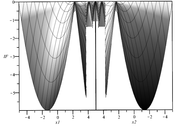
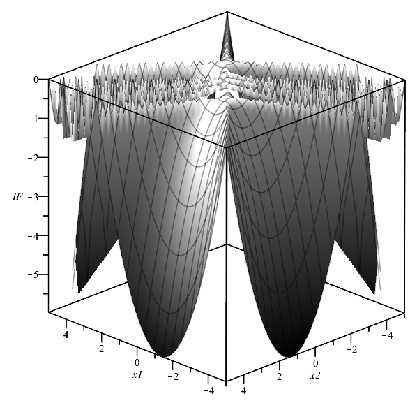
Below we provide some example influence plots to visually demonstrate the effect of a contaminant on the e.d.r direction and the e.d.r space estimators. Consider the linear model
| (13) |
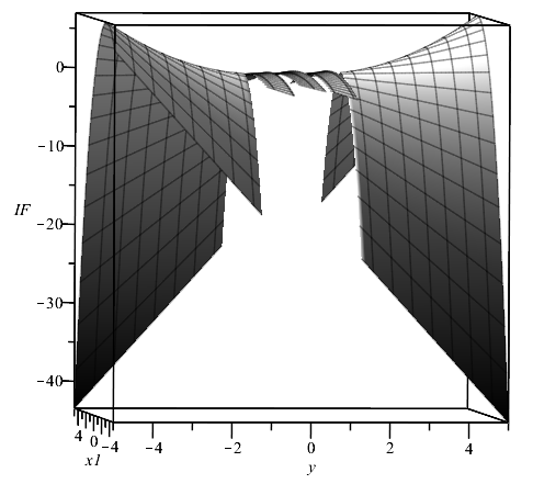
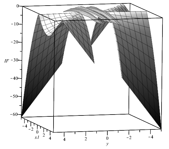
with , , , and equally probable slices. Let IF denote the influence value of the contaminant on the first element of the e.d.r direction given by SWAR. In Figure 1, plot (a) is the and plot (b) is , where for , we set and allow for and to vary. In both plots there is zero influence on the estimators when is also zero, which is expected as explained in Case 1. Within each slice, as and increase, the influence on in plot (a) increases without bound along the diagonal, that is when moves towards the boundaries that determine the slice sub-ranges. In plot (b) of Figure 1, the influence on the e.d.r space follows the same trends as in plot (a) but we also observe approximately zero influence values when follows the model approximately, i.e. when since .
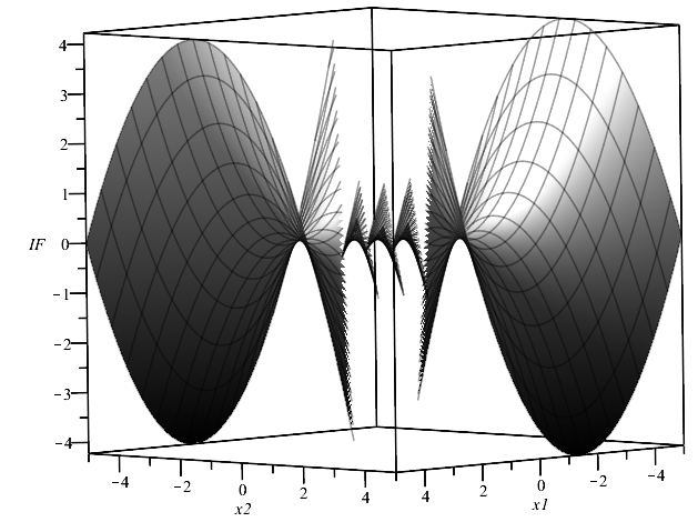
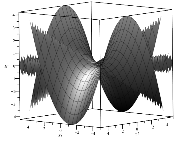
In Figure 2 and 3 we provide two different views for each of the and , respectively, where for the model in (13) we let the response contaminant be consistent with the model, i.e. , and vary and . In both Figures the influence on the estimators is zero when , as expected. Now, for the model in (13), is an element of for any where . Therefore, when then we expect to have zero influence on both estimators, as explained in Case 2 earlier. This is clearly shown in plots (b) of Figure 2 and 3. Furthermore, due to the nature of the model, , when both and increase simultaneously, for example, from 0 to 5, or when their difference is fairly small, then we fall in the middle slices where the influence is relatively small. Although influence still increases within those slices as we reach their limits. The influence increases (towards the far positive or negative values) without bound when the absolute value of the difference () is large.
4.4 Sample and Empirical influence functions
In the sample setting, the influence of the th observation is found by considering the change of the estimator pre- and post-removal of the observation. For a sample of size denoted by , denote the empirical distribution by and the empirical distribution without the th observation by . Then, the sample influence function (SIF) of an estimator with functional is given by . Therefore, the SIF for the SWAR e.d.r direction estimator, with functional , at is given by,
| (14) |
for . Hence, large values in the components of the vector indicate that observation is highly influential.
Similarly, for Bénasséni’s measure, let and denote the matrices whose columns are the estimated e.d.r directions at and . Then, the sample influence function for for the th observation at is
| (15) |
It is clear that when is large, then the th observation is highly influential on the basis that is estimating the CDRS.
The disadvantage of the SIF is that it requires estimates in order to obtain the sample influence values for the entire sample which can be computationally expensive especially when and/or are large. To overcome this, the empirical influence function (EIF) is an approximation of the SIF and can be found by replacing the population parameters of the IF with their sample estimates. Hence, the EIF of the th observation for for SWAR is
| (16) |
where belongs in the th slice. For large , EIF SIF and it can be used in practise to efficiently detect influential observations. Below we provide a comparison between the SIF and EIF of Bénasséni’s measure for SWAR.

5 Some applications of the influence function
The usefulness of the IF expands further than just being a tool to explore the robustness properties of an estimator. In this section, we propose using the mean influence to choose optimal weights for the slices in SWAR, as well as choosing and .
Our first goal is to down-weigh the slices with high mean influence allowing the slices with more stable estimates to contribute more to SWAR. We consider two different weighting techniques: namely, the within slice mean influence and the total mean influence. Detailed explanations for each of these are given below.
5.1 Within slice mean influence weights
Let denote the matrix whose th row is . Also, let denote the th slice slope vector without the th observation and be the matrix whose rows are the ’s that fall in the th slice. For this version of weighting, we consider influence on the dimension reduced predictors within the th slice, and where the dimension reduction has been carried out using the estimated slope vectors within that slice. Similar approach to determining influential observations have been considered previously (Prendergast 2008; Prendergast and Smith 2010, e.g.). For each of the observations within the th slice, compute
| (17) |
Now, let be the mean of the s. Then, the new weights are defined as follows,
| (18) |
and where these are scaled to sum to one.
From here onwards, this version of SWAR which uses the within slice mean influence weights, given in (18), will be referred to as SWARW.
5.2 Total mean influence weights
For this is a re-weighting process first calculate the SWAR estimate (see Section 3) and then calculate the SIF in (15) for each of the observations. Now, let denote the SIFs for the observations in the th slice and the absolute sample mean of these values. Then, the total mean influence weights are given by,
| (19) |
We then recompute the SWAR estimate but where these weights are used instead. The new re-weighted SWAR method with the total mean influence weights will be referred to as SWART.
It is important to note that for SWARW and SWART, the term is used in the weights so that the th slice slope vectors are normalised. This is because only the direction of the vectors is important here and a vector with large length can dominate the dimension reduction matrix and affect the e.d.r direction estimates. Therefore, transforming the slope vectors to have unit length solves this problem.
5.3 Choosing and in SWAR
Influence functions can have multiple applications in the dimension reduction setting. Another application is that of choosing dimension reduction parameters (i.e. and ) based on minimum mean influence, for example. Such applications have been explored in Shaker 2013, and a similar approach has been presented by Ye and Weiss 2003 and Liquet and Saracco 2008; Liquet and Saracco 2012, who evaluated the sensitivity of dimension reduction estimators at different parameter values using a bootstrap approach.
In the mean influence approach, which we adopt here, we consider the optimal pair , to be the one that results in the minimum mean influence. For SWAR, the sample influence function of Bénasséni’s measure can be used to select in conjunction with . An example of this, for a simulated model, is given soon in Section 6. An inspection of the Estimated SSPs (ESSPs) is also recommended when choosing and in practice.
The only disadvantage of the mean SIF compared to the bootstrap approaches is the computational intensity of the SIF. However, for large sample sizes where EIF SIF, the EIF can be used in practice to choose and more efficiently, since computational intensity reduces significantly. The HIF (Prendergast 2007) provides another alternative to the SIF which can provide a better approximation than the EIF and is also less time consuming than the SIF. The effectiveness of the SIF in choosing and is not examined thoroughly in the present paper.
6 Simulations
In this section, we provide simulated examples to demonstrate the effectiveness of SWAR, SWARW and SWART. The performance of the aforementioned methods is compared with those of OLS, PALS and SIR and results provided. We have chosen principal asymmetric least squares (Soale and Dong 2022, PALS,) since it is an interesting new method that also combines least squares estimates. The PALS object function is
where and where is the asymmetric least squares loss function (Newey and Powell 1987). For given values for , a slope using the above objective function is computed (estimated on the standardised scale and pre-multiplied by ), and combined similarly to our Step 4 of SWAR but with weights all equal to one.
For every model, we perform 1000 repetitions for each combination of the sample sizes and with and , and and for the slicing methods. For PALS we follow the lead of Soale and Dong 2022 and set the tuning parameter and . To measure and evaluate the performance of each method we use the squared canonical correlations between the true and estimated e.d.r spaces.
6.1 Single-Index Model
Consider the following model with independent of and ,
Model 1 ,
where the true .

For this model we first perform the aforementioned methods for each combination of and . Then, we introduce contamination and perform the same comparisons to see where the influence weighting strategies can improve estimation. We then replace of the ordered observations based on the value of with contamination, where the contamination response is generated from and we subtract five from each of the associated predictor vector elements.
To highlight the effect of this type of contamination, we first provide some example ESSPs in Figure 5 for and . The contamination is clearly evident in the true ESSP (i.e. assuming known ). However, from the estimated ESSPs using OLS and SWAR, we can no longer distinguish these points from other observations. However, the estimated ESSP using SWART provides an excellent estimate of the ESSP. Hence we have chosen this type of contamination since resulting ESSPs may provide no indication that some problematic observations need further inspection.
Uncontaminated Method OLS 0.953 (0.034) 0.900 (0.051) 0.811 (0.062) 0.986 (0.010) 0.969 (0.016) 0.936 (0.023) 0.994 (0.004) 0.986 (0.007) 0.972 (0.010) PALS () 0.947 (0.039) 0.890 (0.057) 0.802 (0.066) 0.983 (0.012) 0.962 (0.020) 0.925 (0.029) 0.993 (0.005) 0.983 (0.009) 0.965 (0.014) SIR () 0.949 (0.033) 0.890 (0.046) 0.796 (0.055) 0.987 (0.009) 0.971 (0.014) 0.941 (0.017) 0.995 (0.003) 0.988 (0.005) 0.976 (0.008) SIR () 0.984 (0.012) 0.962 (0.020) 0.921 (0.031) 0.996 (0.003) 0.992 (0.004) 0.983 (0.006) 0.999 (0.001) 0.997 (0.001) 0.993 (0.002) SIR () 0.988 (0.009) 0.972 (0.016) 0.937 (0.031) 0.998 (0.002) 0.995 (0.003) 0.989 (0.004) 0.999 (0.001) 0.998 (0.001) 0.996 (0.001) SWAR () 0.967 (0.029) 0.914 (0.063) 0.641 (0.215) 0.992 (0.006) 0.982 (0.010) 0.960 (0.017) 0.997 (0.002) 0.993 (0.004) 0.984 (0.006) SWAR () 0.863 (0.168) 0.983 (0.014) 0.957 (0.028) 0.875 (0.069) 0.994 (0.005) 0.985 (0.008) 0.966 (0.014) SWAR () 0.956 (0.053) 0.848 (0.132) 0.986 (0.011) 0.966 (0.021) 0.909 (0.046) SWARW () 0.980 (0.017) 0.942 (0.039) 0.709 (0.192) 0.995 (0.004) 0.988 (0.006) 0.972 (0.011) 0.998 (0.002) 0.995 (0.003) 0.989 (0.004) SWARW () 0.960 (0.075) 0.998 (0.002) 0.994 (0.005) 0.982 (0.014) 0.999 (0.001) 0.998 (0.001) 0.996 (0.002) SWARW () 0.993 (0.007) 0.978 (0.036) 0.998 (0.002) 0.995 (0.003) 0.987 (0.007) SWART () 0.966 (0.033) 0.910 (0.071) 0.656 (0.214) 0.988 (0.009) 0.975 (0.015) 0.944 (0.026) 0.995 (0.004) 0.988 (0.006) 0.975 (0.011) SWART () 0.943 (0.147) 0.996 (0.017) 0.987 (0.051) 0.968 (0.087) 0.999 (0.001) 0.998 (0.003) 0.996 (0.006) SWART () 0.936 (0.147) 0.901 (0.169) 0.975 (0.084) 0.965 (0.088) 0.937 (0.121)
Contaminated Method OLS 0.308 (0.190) 0.289 (0.170) 0.238 (0.145) 0.337 (0.110) 0.301 (0.108) 0.271 (0.097) 0.340 (0.077) 0.297 (0.073) 0.275 (0.067) PALS () 0.321 (0.193) 0.301 (0.171) 0.244 (0.146) 0.357 (0.113) 0.320 (0.111) 0.285 (0.099) 0.362 (0.080) 0.320 (0.077) 0.296 (0.070) SIR () 0.785 (0.071) 0.720 (0.068) 0.627 (0.072) 0.812 (0.033) 0.773 (0.033) 0.732 (0.034) 0.816 (0.021) 0.784 (0.021) 0.758 (0.022) SIR () 0.773 (0.062) 0.737 (0.061) 0.687 (0.068) 0.788 (0.029) 0.754 (0.030) 0.726 (0.031) 0.789 (0.019) 0.755 (0.019) 0.733 (0.020) SIR () 0.741 (0.069) 0.707 (0.068) 0.661 (0.074) 0.762 (0.031) 0.723 (0.033) 0.694 (0.034) 0.766 (0.020) 0.723 (0.021) 0.698 (0.022) SWAR () 0.382 (0.203) 0.404 (0.182) 0.285 (0.170) 0.441 (0.112) 0.461 (0.104) 0.463 (0.092) 0.449 (0.077) 0.467 (0.070) 0.480 (0.062) SWAR () 0.401 (0.233) 0.454 (0.117) 0.471 (0.112) 0.429 (0.117) 0.470 (0.074) 0.504 (0.068) 0.518 (0.060) SWAR () 0.473 (0.181) 0.379 (0.177) 0.502 (0.100) 0.491 (0.094) 0.451 (0.100) SWARW () 0.951 (0.064) 0.879 (0.122) 0.562 (0.257) 0.948 (0.050) 0.878 (0.093) 0.825 (0.102) 0.960 (0.029) 0.900 (0.052) 0.854 (0.068) SWARW () 0.916 (0.147) 0.984 (0.035) 0.970 (0.037) 0.944 (0.059) 0.992 (0.008) 0.983 (0.016) 0.973 (0.021) SWARW () 0.976 (0.058) 0.955 (0.055) 0.991 (0.011) 0.982 (0.020) 0.969 (0.028) SWART () 0.954 (0.057) 0.895 (0.103) 0.605 (0.253) 0.990 (0.009) 0.977 (0.019) 0.954 (0.026) 0.996 (0.004) 0.991 (0.006) 0.982 (0.011) SWART () 0.900 (0.198) 0.988 (0.055) 0.976 (0.071) 0.954 (0.091) 0.997 (0.007) 0.996 (0.004) 0.992 (0.010) SWART () 0.880 (0.196) 0.853 (0.207) 0.932 (0.153) 0.924 (0.145) 0.884 (0.188)
The averages of the squared correlations along with their corresponding standard deviations, shown in parentheses, for the uncontaminated and contaminated Model 6.1, are given in Table 1. The missing values (denoted by ) for SWAR, SWARW and SWART in the tables are for when so that slopes cannot be estimated. Figure 6, shows the box-plots of the correlations from 1000 repetitions of each method for . For simplicity, the results for are omitted from the table and the box-plots since they display similar trends with .

We can see that all methods perform extremely well for the uncontaminated case, especially as the sample size increases. OLS and PALS tend to perform better than SWAR methods when the sample size is small and dimensionality is large (e.g., and ). SIR is also better than SWAR for small sample sizes but performance is similar for larger . Whereas SIR’s performance is better when the number of slices is large, all versions of SWAR prefer a smaller or intermediate number of slices.
For the contaminated Model 6.1, the performance of OLS and PALS deteriorates significantly. SWAR also performs poorly, but to a lesser degree, and SIR provides reasonable estimates but still a notable decrease in performance. However, the weighted adjusted methods SWARW and SWART show an outstanding performance in the presence of contamination, which was shown by example in Figure 5 for SWART.
| 918 | 1000 | 988 | 760 | 905 | 995 | 637 | 799 | 941 | 515 | 686 | 862 | ||
| 82 | 186 | 83 | 5 | 298 | 183 | 57 | 403 | 274 | 133 | ||||
| 54 | 12 | 65 | 18 | 2 | 82 | 40 | 5 | ||||||
| 0 | 0 | 12 | 0 | 0 | 0 | 0 | 0 | 0 | 0 | 0 | 0 | ||
| 0 | 0 | 0 | 0 | 0 | 0 | 0 | 0 | 0 | 0 | ||||
| 0 | 0 | 0 | 0 | 0 | 0 | 0 | 0 | ||||||
Finally, Table 2 shows how many times (out of 1000 repetitions) the SIF given in (15) has chosen each pair of and for SWAR, for the uncontaminated Model 6.1. Between the choice of and , the SIF is correctly choosing in all replications except for and for which case the method is struggling to find a good estimate. For the optimal number of slices is chosen the most. This is consistent with the previous findings that SWAR prefers a smaller number of slices. As increases, a larger number of slices is often chosen.
6.2 Multiple-Index model
Similarly to the previous example, for independent of with , consider now
Model 2 ,
with true e.d.r directions, and .
| Method | |||||||||
| PALS () | 0.668 (0.381) | 0.577 (0.417) | 0.508 (0.421) | 0.722 (0.341) | 0.617 (0.403) | 0.560 (0.435) | 0.786 (0.288) | 0.680 (0.354) | 0.598 (0.410) |
| PALS () | 0.772 (0.301) | 0.667 (0.354) | 0.583 (0.393) | 0.915 (0.131) | 0.829 (0.202) | 0.729 (0.282) | 0.960 (0.061) | 0.906 (0.114) | 0.828 (0.188) |
| SIR () | 0.510 (0.471) | 0.489 (0.436) | 0.455 (0.384) | 0.512 (0.485) | 0.513 (0.472) | 0.514 (0.446) | 0.513 (0.487) | 0.517 (0.481) | 0.528 (0.463) |
| SIR () | 0.763 (0.312) | 0.638 (0.370) | 0.545 (0.398) | 0.932 (0.108) | 0.852 (0.178) | 0.752 (0.261) | 0.976 (0.036) | 0.940 (0.073) | 0.880 (0.127) |
| SIR () | 0.746 (0.329) | 0.617 (0.393) | 0.529 (0.422) | 0.930 (0.123) | 0.843 (0.200) | 0.736 (0.290) | 0.978 (0.033) | 0.945 (0.066) | 0.888 (0.121) |
| SWAR () | 0.905 (0.168) | 0.807 (0.242) | 0.589 (0.353) | 0.972 (0.054) | 0.935 (0.090) | 0.867 (0.157) | 0.988 (0.022) | 0.970 (0.043) | 0.936 (0.078) |
| SWAR () | 0.924 (0.158) | 0.987 (0.032) | 0.961 (0.072) | 0.884 (0.170) | 0.994 (0.011) | 0.984 (0.027) | 0.961 (0.059) | ||
| SWAR () | 0.977 (0.060) | 0.904 (0.177) | 0.988 (0.026) | 0.966 (0.062) | 0.900 (0.154) | ||||
| SWARW () | 0.905 (0.168) | 0.807 (0.242) | 0.589 (0.353) | 0.972 (0.054) | 0.935 (0.090) | 0.867 (0.157) | 0.988 (0.022) | 0.970 (0.043) | 0.936 (0.078) |
| SWARW () | 0.934 (0.154) | 0.993 (0.011) | 0.979 (0.028) | 0.930 (0.098) | 0.997 (0.005) | 0.992 (0.010) | 0.980 (0.022) | ||
| SWARW () | 0.990 (0.034) | 0.954 (0.102) | 0.997 (0.005) | 0.992 (0.010) | 0.976 (0.032) | ||||
| SWART () | 0.905 (0.168) | 0.807 (0.242) | 0.589 (0.353) | 0.972 (0.054) | 0.935 (0.090) | 0.867 (0.157) | 0.988 (0.022) | 0.970 (0.043) | 0.936 (0.078) |
| SWART () | 0.795 (0.305) | 0.955 (0.103) | 0.869 (0.208) | 0.687 (0.350) | 0.988 (0.021) | 0.962 (0.067) | 0.902 (0.138) | ||
| SWART () | 0.743 (0.348) | 0.584 (0.410) | 0.871 (0.244) | 0.726 (0.347) | 0.578 (0.420) | ||||

The average values of the squared canonical correlations with the corresponding standard deviations, in parentheses, can be found in Table 3. The box-plots of the squared canonical correlations for are then given in Figure 7. In the boxplots, we provide the squared canonical correlations for each direction so that we can compare performance for both directions.
For this model, PALS with fails to find a second direction, however, a different value of the tuning parameter seems to improve the results significantly especially as increases. Therefore, this model is an example case where can have a significant effect on estimation, a perhaps unexpected result based on analysis carried out about PALS so far, where did not have a significant effect on estimation (Soale and Dong 2022). SIR struggles to find a good estimate of the subspace when is small (for this is expected since the SIR matrix is of rank 1), and it can often find it difficult to estimate the second direction unless is large, as is evident in the box-plots.
All SWAR versions perform comparatively well even when the sample size is small, in which case there is more variability in the estimation of the second direction. The performance of the SWAR methods also declines slightly when increases. Additionally, SWAR and SWART benefit from a small to intermediate choice of , whereas SWARW benefits from an intermediate to a larger number of slices.
7 BigMac data example
In this section we compare the estimated directions given by OLS, SIR, SWAR, SWARW and SWART for the ‘BigMac’ data from Enz 1991. Of interest is the regression of the response, the minimum labor required to buy a Big Mac and fries from MacDonalds in each city, on the 9 socio-economic predictor variables. There are 45 observations in the data and so we choose for SIR and for SWAR, SWARW and SWART we choose . These choices of was confirmed to be the most suited to each method through the inspection of the Estimated SSPs (ESSPs). Inspections of ESSPs also revealed that was suitable.

The ESSPs for each method are shown in Figure 8 where an exponential curve has been added to each plot. It is evident from Figure 8 that SWAR provides the best ESSP for the BigMac data with the curve fitting all observations reasonably well. OLS performs comparatively poorly, SIR performs well except for a notable outlier that does not fit well, and SWARW also provides a good fit.
8 Discussion
In this paper we consider slice weight average regresion (SWAR), along with robustified versions of this method using influence re-weighting (SWARW and SWART). These versions utilize the mean sample influence function to down-weight the slices that contain highly influential observations which therefore provide a non-robust estimate. This weighting process can also be easily applied to other dimension reduction methods that combine multiple vectors into a dimension reduction matrix. Although not reported here, we also considered re-weighted versions of SIR and PALS but with no notable improvements (some slight improvements for PALS was detected).
Despite the fact the OLS can only be used for a single direction , SWAR method is surprisingly capable of finding a second direction for the models we considered.
Acknowledgments. We are very grateful to Abdul-Nasah Soale and Yuexiao Dong for kindly providing the implementation code for PALS.
Declarations
Funding. This research is funded by the Australian Government’s Research Training Program (RTP) in support of MM’s doctoral research degree at La Trobe University. The funding body had no role in the reported research and in writing the manuscript.
Code availability. R codes are available from the corresponding author upon request.
Data availability. The public data set, used in this article, and additional information can be found at https://www.rdocumentation.org/packages/ldr/versions/1.3.3/topics/bigmac .
Conflicts of interest. The authors have no conflicts of interest to declare that are relevant to the content of this article.
Appendix A Proof of Lemma 1
Let , be any subrange of the range of and, for simplicity in what follows, . First, from Lemma 1 of Prendergast 2007, when Conditions 1 and 2 hold,
| (20) |
Also, from Prendergast 2005, under Condition 1
| (21) |
Then, it is simple to show, from the Woodbury matrix identity (Woodbury 1950), that,
| (22) |
Furthermore, by conditioning and (21), we get,
| (23) |
for any range of , since due to the independence between and .
Appendix B Influence functions derivations for SWAR
B.1 Influence functions for the SWAR matrix and the single-index model e.d.r. direction
Let and denote the functionals for the th slice covariance matrices so that at , and respectively. In addition, let denote the functional of the th slice slope vector estimator where . For simplicity, we let and . From Prendergast 2007,
| (24) |
Since , using the Product Rule and by setting to 0 we have, . Then, from (24), the influence function for the inverse slice variance is
| (25) |
For brevity here we omit the details, but by following closely the proof for (24) (Prendergast 2007, see Lemma A1 proof of), we have
| (26) |
Let denote the function for the SWAR matrix estimator such that . Using the Product Rule, the influence function for is straightforward when using (27). We present the result in the following lemma for use later.
Lemma 2.
Under Assumption 1, the influence function of the SWAR dimension reduction matrix estimator, with functional , at is given by,
| (28) |
where is the OLS residual of in the th slice, , and and are the means of the ’s and the ’s in the th slice, respectively.
Eq. 13 of Prendergast 2005 provides the influence functions for the eigenvectors of the SIR matrix estimator and this result can be adapted and used directly here. However, from Lemma 2 and in the case , the influence functions for SWAR e.d.r. direction estimators depend on the expressions involving and which cannot be derived further. We therefore focus our attention on the case of . This is of the form, since for ,
| (29) |
The form of the IF in the case of simplifies due to several results which we list here: (i) from Lemma 1, we have that for some . Since is also a scalar multiple of , then for (since ); (ii) from (22), we know that for a . Therefore, ; (iii) from (20) and (A), and , . Hence, using (i)-(iii), only the first term of IF in Lemma 2 remains in (29).
The proof of Theorem 2 is complete when applying (ii) to this first term also.
B.2 Proof of Theorem 4
From Bénasséni 1990 the influence function for , with respect to SWAR, is of the form,
| (30) |
Note that, is a projection matrix on the compliment of the CDRS. Hence, similar to the proof for Theorem 2 where we noted several simplifications, firstly we have . Secondly, since , then using (A) for the form of for any range
It can similarly be shown that
by using the form of the slice variance matrix in (20). Then, the proof is complete by substituting (2) in (30) and using the above simplifications.
Appendix C Proof of ASV
Since is a function of and , and is independent of , then by conditioning we can write From (21) and since , we can write
| (32) |
Note that the term on the righthand side of (32) is which, from Eq. 4 of Prendergast 2007, is equal to . Therefore, (32) simplifies to just which completes the proof.
References
- Bellman (1961) Bellman, R. Adaptive Control Processes. Princeton University Press, Princeton, NJ., 1961.
- Bénasséni (1990) Bénasséni, J. Sensitivity coefficients for the subspaces spanned by principal components. Commun. Stat. - Theory Methods, 19:2021–2034, 1990.
- Brillinger (1977) Brillinger, D. R. The identification of a particular nonlinear time series system. Biometrika, 64:509–515, 1977.
- Brillinger (1983) Brillinger, D. R. A genralized linear model with “Gaussian" regressor variables. A Festschrift For Eric L. Lehmann, Wadsworth Statist. /Probab. Ser. Belmont, CA: Wadsworth, pages 97–114, 1983.
- Clarke (2018) Clarke, B. R. Robustness theory and application. John Wiley & Sons, Hoboken, NJ, 2018.
- Cook (1998) Cook, R. D. Regression graphics. Ideas for studying regressions through graphics. New York: John Wiley & Sons Inc., 1998. ISBN 0-471-19365-8.
- Cook (2007) Cook, R. D. Fisher lecture: Dimension reduction in regression. Stat. Sci., 22(1):1–26, 2007. ISSN 08834237.
- Cook and Forzani (2008) Cook, R. D. and Forzani, L. Principal fitted components for dimension reduction in regression. Stat. Sci., 23(4):485–501, 2008. ISSN 08834237.
- Cook and Forzani (2009) Cook, R. D. and Forzani, L. Likelihood-based sufficient dimension reduction. J. Am. Stat. Assoc., 104(485):197–208, 2009. URL https://doi.org/10.1198/jasa.2009.0106.
- Cook and Weisberg (1991) Cook, R. D. and Weisberg, S. Sliced inverse regression for dimension reduction: Comment. J. Am. Stat. Assoc., 86:328–332, 1991. ISSN 01621459.
- Eaton (1986) Eaton, M. L. A characterization of spherical distributions. J. Multiv. Anal., 20(2):272–276, 1986. URL https://doi.org/10.1016/0047-259X(86)90083-7.
- Enz (1991) Enz, R. Prices and Earnings Around the Globe. Zurich: Union Bank of Switzerland, 1991.
- Garnham and Prendergast (2013) Garnham, A. L. and Prendergast, L. A. A note on least squares sensitivity in single-index model estimation and the benefits of response transformations. Electron. J. Stat., 7:1983–2004, 2013. URL https://doi.org/10.1214/13-EJS831.
- Gather et al. (2002) Gather, U.; Hilker, T., and Becker, C. A note on outlier sensitivity of sliced inverse regression. Statistics, 36(4):271–281, 2002. URL https://doi.org/10.1080/02331880213194.
- Hall and Li (1993) Hall, P. and Li, K.-C. On almost Linearity of Low Dimensional Projections from High Dimensional Data. Ann. Stat., 21(2):867–889, 1993. URL https://doi.org/10.1214/aos/1176349155.
- Hampel (1974) Hampel, F. R. The influence curve and its role in robust estimation. J. Am. Stat. Assoc., 69:383–393, 1974. ISSN 01621459. URL http://www.jstor.org/stable/2285666.
- Hampel (1986) Hampel, F.R. Robust statistics : the approach based on influence functions. Wiley series in probability and mathematical statistics. Probability and mathematical statistics. Wiley, New York, 1986. ISBN 0471829218.
- Li et al. (2011) Li, B.; Artemiou, A., and Li, L. Principal support vector machines for linear and nonlinear sufficient dimension reduction. Ann. Stat., 39(6):3182 – 3210, 2011. URL https://doi.org/10.1214/11-AOS932.
- Li (1991) Li, K.-C. Sliced inverse regression for dimension reduction. J. Am. Stat. Assoc., 86:316–327, 1991. doi: 10.1080/01621459.1991.10475035.
- Li (1992) Li, K.-C. On Principal Hessian Directions for Data Visualization and Dimension Reduction: Another Application of Stein’s Lemma. J. Am. Stat. Assoc., 87:1025–1039, 1992. ISSN 01621459. URL http://dx.doi.org/10.2307/2290640.
- Li and Duan (1989) Li, K.-C. and Duan, N. Regression Analysis Under Link Violation. Ann. Stat., 17:1009–1052, 1989. URL https://doi.org/10.1214/aos/1176347254.
- Liquet and Saracco (2008) Liquet, B. and Saracco, J. Application of the bootstrap approach to the choice of dimension and the parameter in the sirα method. Commun. Stat. - Simul. Comput., 37(6):1198–1218, 2008. URL https://doi.org/10.1080/03610910801889011.
- Liquet and Saracco (2012) Liquet, B. and Saracco, J. A graphical tool for selecting the number of slices and the dimension of the model in SIR and SAVE approaches. Comput. Stat., 27(1):103–125, April 2012. URL https://doi.org/10.1007/s00180-011-0241-9.
- Newey and Powell (1987) Newey, W. K. and Powell, J. L. Asymmetric least squares estimation and testing. Econometrica: Journal of the Econometric Society, pages 819–847, 1987.
- Prendergast (2005) Prendergast, L. A. Influence functions for sliced inverse regression. Scand. J. Stat., 32(3):385–404, sep 2005. URL https://doi.org/10.1111/j.1467-9469.2005.00447.x.
- Prendergast (2007) Prendergast, L. A. Implications of influence function analysis for sliced inverse regression and sliced average variance estimation. Biometrika, 94(3):585–601, 2007. ISSN 00063444.
- Prendergast (2008) Prendergast, L. A. Trimming influential observations for improved single-index model estimated sufficient summary plots. Comput. Stat. Data Anal., 52:5319–5327, 2008. doi: 10.1016/j.csda.2008.05.014.
- Prendergast and Garnham (2016) Prendergast, L. A. and Garnham, A. L. Response and predictor folding to counter symmetric dependency in dimension reduction. Aust. N-Z. J. Stat., 58(4):515–532, 2016. doi: https://doi.org/10.1111/anzs.12170.
- Prendergast and Smith (2010) Prendergast, L. A. and Smith, J. A. Influence functions for dimension reduction methods: An example influence study of principal hessian direction analysis. Scand. J. Stat., 37:588–611, 2010. ISSN 03036898, 14679469.
- Shaker (2013) Shaker, A. Combining dimension reduction methods. PhD thesis, La Trobe University, Melbourne, Australia, 2013.
- Sheather and McKean (2001) Sheather, S. J. and McKean, J. W. Discussion on special invited paper: Dimesion reduction and visualization in discriminant analysis. Aust. N.Z.J. Stat., 43(2):185–190, 2001.
- Soale and Dong (2022) Soale, A-N. and Dong, Y. On sufficient dimension reduction via principal asymmetric least squares. J. Nonparametr. Stat., 34(1):77–94, 2022. URL https://doi.org/10.1080/10485252.2021.2025237.
- Wang et al. (2018) Wang, C.; Shin, S. J., and Wu, Y. Principal quantile regression for sufficient dimension reduction with heteroscedasticity. Electron. J. Stat., 12(2):2114 – 2140, 2018. URL https://doi.org/10.1214/18-EJS1432.
- Woodbury (1950) Woodbury, M. A. Inverting modified matrices. Statistical Research Group, Memo. Rep. 42, Princeton University, Princeton, N. J, 1950.
- Xia et al. (2002) Xia, Y.; Tong, H.; Li, W. K., and Zhu, L-X. An adaptive estimation of dimension reduction space. J. R. Stat. Soc. Series B - Stat. Methodol., 64(3):363–410, 2002. ISSN 13697412, 14679868.
- Ye and Weiss (2003) Ye, Z. and Weiss, R. E. Using the bootstrap to select one of a new class of dimension reduction methods. J. Am. Stat. Assoc., 98:968–979, 2003. URL https://doi.org/10.1198/016214503000000927.
- Yin and Cook (2004) Yin, X. and Cook, R. D. Dimension reduction via marginal fourth moments in regression. J. Comput. Graph. Stat., 13(3):554–570, 2004. URL https://doi.org/10.1198/106186004X2462.
- Zhu et al. (2007) Zhu, L.-X.; Ohtaki, M., and Li, Y. On hybrid methods of inverse regression-based algorithms. Comput. Stat. Data Anal, 51(5):2621–2635, 2007. ISSN 0167-9473. URL https://doi.org/10.1016/j.csda.2006.01.005.