Low-temperature electron mobility in doped semiconductors with high dielectric constant
Abstract
We propose and study theoretically a new mechanism of electron-impurity scattering in doped seminconductors with large dielectric constant. It is based upon the idea of vector character of deformations caused in the crystalline lattice by any point defects siting asymmetrically in the unit cell. In result, local lattice compression due to the elastic deformations decay as with distance from impurity. Electron scattering (due to standard deformation potential) on such defects leads to low-temperature mobility scaling with electron density of the form that is close to experimental observations on a number of relevant materials.
Introduction A number of doped semiconductors is known to demonstrate low-temperature mobility with a nearly power-law dependence on electron density, , with the exponent in the interval , see Ref. STO1; STO2; STO3; STO4; STO5 for Strontium Titanate SrTiO3, Ref. KTO for Potassium Tantalate KTaO3, Ref. STO1; PbTe1; PbTe2 for Lead Telluride PbTe and Ref. TlBiSSe for mixed-chalcogenide compound TlBiSSe. Obviously, mobility in the should be determined by impurity scattering, but it is not so easy to identify the specific mechanism of this scattering. Indeed, an obviously existing scattering by screened Coulomb potentials produced by charged impurities leads Coulomb; Hamaguchi to . Another omnipresent type of scattering is provided by short-range random potentials, but this one leads to density - independent scattering cross-section, thus . None of these mechanisms is able to explain the data STO1; STO2; STO3; STO4; STO5; KTO; PbTe1; PbTe2. The common feature of all these doped semiconductors is high dielectric constant of the corresponding undoped material, which makes Coulomb scattering by charged impurities very weak.
In the present manuscript we propose and study a new mechanism of electron scattering by point defects, which we call vector impurity mechanism. Our key idea follows from two observations: i) all considered families of semiconductors have crystal lattices with relatively complicated elementary cells, which forces lattice defects (a vacancy or a substitutional atom) to break down the symmetry of elastic media around it; as a result, such defects act as a microscopic ”force” upon surrounding elastic media. ii) elastic deformations due to a point-like force applied to an elastic media leads LL7 to lattice deformations with slowly decaying compression . Now, one can employ usual electron-phonon deformation potential Hamiltonian of the form to find that it leads to the impurity transport cross-section , with being transfered momentum. With typical , one immediately find mobility which is rather close to the observations STO1; STO2; STO3; STO4; STO5; KTO; PbTe1; PbTe2. Below we provide detailed exposition of our approach, and apply it first to Strontium Titanate (where some complications arise due to its many-band structure), and then to KTaO3, PbTe and TlBiSSe.
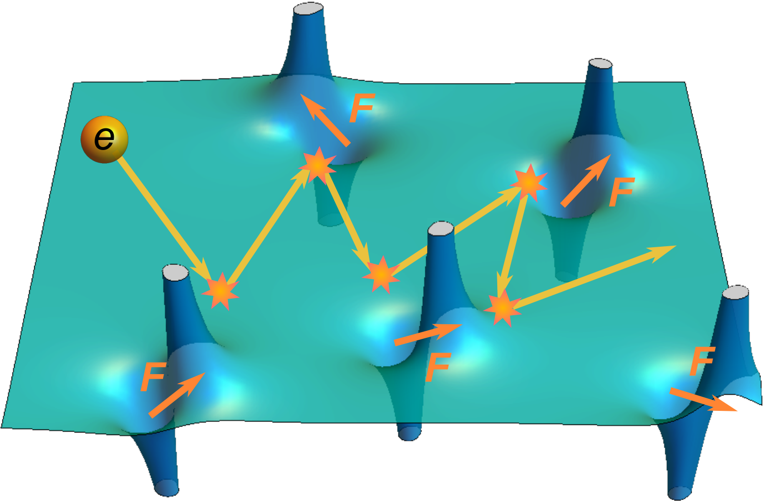
Elastic deformations due to vector impurities. Conduction-band electrons in semiconductors interact with lattice distortions via deformation potential
| (1) |
where coupling constant is usually rather large, about few eV. Thus we need to consider possible sources of lattice distortions leading to non-zero compression . In the simplest model of a ”void” in isotropic elastic media, the deformations which arise around it lead to , see LL7, Problem 2 for Paragraph 7. Crucial point is to notice that any atomic defect in a complicated crystal structure will break the symmetry of the lattice in the way that is equivalent to the presence of some local vector source. In other words, it would be incorrect to consider Oxygen vacancy in STO just as small spherical defect in elastic media, as it would be possible in case of vacancy is simple cubic lattice with single atom per unit cell. Oxygen defects in the lattice of STO are located asymmetrically w.r.t. center of the unit cell. Thus, in terms of symmetry of elastic deformation, the effect of such a defect is equivalent to the presence of some frozen in local force . The problem of elastic deformations in the presence of such a force was first solved by W.Thomson in 1848; detailed solution is present in Ref.LL7, as the Problem to the Paragraph 8. It reads as follows:
| (2) |
Here and are the Poisson’s ratio and Young modulus respectively, the magnitude of a force will serve as a fitting parameter for our theory. Local compression corresponding to deformations (2) is given by
| (3) |
Fig. 1 presents a sketch of electron scattering on a random deformation potential caused by vector impurities.
Collision integral, relaxation time and mobility. Now we use the Hamiltonian (1) with impurity-induced compressions given by Eq.(3) to calculate electron scattering rates.
We will study electric transport in an electron system using the Boltzmann kinetic equation. To find the conductivity and the corresponding mobility within linear response theory, we expand the distribution function as . Where, is the Fermi-Dirac distribution with and Boltzmann constant , and with the Fermi energy . Since we are concerned with the low-temperature transport we will limit our discussions for , thus in the leading order approximating the Fermi-Dirac distribution with a step function. This helps to write the Boltzmann equation in presence of electric field in the linearized form:
| (4) |
where is the group velocity. The collision integral in the RHS of the above equation describes the electron scattering at the impurity-induced compressions governed by the Eq.(3). It is explicitly expressed as follows
| (5) |
where we introduced a notation , for summation over impurities, and for the Fourier transform of the deformation potential from the Eq.(3) induced by the impurity:
| (6) |
The deviation of the distribution function from the Fermi distribution is produced by the electric field, thus for an isotropic Fermi surface in the limit of weak electric field we can preserve only the first angular harmonics and choose , with the function being only energy dependent. As a result, the integral (5) can be evaluated explicitly, as detailed in Supp, producing:
| (7) | ||||
| (8) |
with denoting a unit vector along the momentum p. We emphasize that the above expression is dependent not only on the relative orientation of momentum p and electric field , but also on the relative orientations of p and the vector force F.
In order to sum over the impurities we need to average the expression (8) over the orientation of the vector F. As a result we obtain a final expression for the collision integral in a form with a relaxation time
| (9) |
The relaxation time is then used to find the electron mobility:
| (10) |
We see that for a concentration independent effective mass electron mobility scales with concentration as as tipped off in the Introduction. However, since the mass enters squared in the above equation, even a relatively weak -dependence can influence the results considerably.
Application to SrTi. One of the most interesting materials that our discussions can be applied to is Strontium Titanate . Being a band insulator it becomes a very dilute 3D metal due to tiny doping ( conduction electrons per unit cell) and demonstrates a number of unusual properties Spinelli2010; review1; review2. They mainly originate form the close proximity of insulating STO to a ferroelectric transition, which leads to a giant low-temperature dielectric constant . As a result, Coulomb interaction in STO is strongly suppressed; the accurate consideration shows that the electron mobility produced by the scattering on Coulomb field is more than two orders of magnitude greater than the experimental data.
Having an almost spherical Fermi surface when lightly doped, at concentrations higher than acquires a complicated multiband Fermi surface far from being isotropic MassSdh; FermiSurf1; FermiSurf2; FermiSurf3; FermiSurf4. Anisotropic Fermi surface can potentially produce correlations between the subsequent scatterings by affecting the scattering direction probability distribution after each act of scattering. This is indeed the case for scattering on isotropic impurities where light electrons can contribute to the collision integral more dramatically than heavy ones. However, according to the Eq. (8) the collision integral depends strongly on the relative orientation of p and the vector force F, and of E and F. Since these vector forces are oriented randomly, the exact shape of the Fermi surface does not seem to be relevant and the electron scattering is effectively averaged out. This enables us to model the electron dynamics with a spherical Fermi surface with an effective mass introduced phenomenologically as
| (11) |
with the Fermi energy obtained from the experimental data. Somewhat similar approach is used in McCalla2019. Fig. 2 summarizes a number of experimental data for the effective mass in the lowest band of STO, obtained by different kinds of experiments: Shubnikov-de Haas effect, quantum oscillations and the density of states (DoS) mass found from specific heat measurements. Continuous green line in the same plot shows the dependence which we extracted using the data from Ref.T^2 for Fermi energy and Eq.(11), to be used in our further calculations.
The above considerations allow us to directly implement the result given by Eq. (10) for the analysis of experimental data on SrTiO3. Fig. 3a) compares our theoretical results for electron mobility with the experimental data STO2. We used here single fit parameter, the strength of vector impurity potential . It shows a reasonable overall scaling with deviations not exceeding for cm-3.
Our approach improperly predicts the mobility behaviour at lowest concentrations where experimental data demonstrate saturation of with further decrease of below cm-3, which is not described by Eq.(10). It means that another scattering process should be taken into account to describe this feature. One possible effect could come from Coulomb interaction which leads to slow logarithmic dependence of . However it is easy to check that Coulomb scattering itself would lead to mobility overestimated by 2 orders of magnitude. Another possible explanation could be electron scattering on domain walls. These processes can be roughly modeled using a relaxation time defined as , where is the characteristic domain size. In order to fit the experimental data for STO this approach requires the domain size to be m, wheres the experiment domain reveals the domain size to be an order of magnitude larger. Finally, we would like to mention spatial non-uniformity of dopant’s concentration as a possible source of saturation at lowest ; we leave investigation of this issue for future research.
Now we need to implement ”sanity check” to see how large are the lattice deformations induced by our vector impurities. Let us evaluate the characteristic displacement at the minimal distance from the impurity, using known parameters of STO, like the deformation potential eV Dac, Young modulus GPa and Poisson ratio Elastic. To describe the experimental data we used a fit parameter N. According to Eq. (2), it corresponds to largest atomic displacement
| (12) |
where nm is the STO lattice constant. Such a maximal displacement does not seem to be unreasonable.
Application to other materials: Now we extend our analysis for several other doped semiconductors with high dielectric constants. Namely, we use our approach to describe electron mobility in a wide-gap semiconductor perovskite Potassium Tantalate KTaO3, Lead Telluride PbTe - narrow gap semicoonductor, and a zero-gap semiconductor - mixed-chalcogenide compound TlBiSSe; their dielectric constants are roughly 4500, 1000 and 20 respectively.
Effective electron mass in PbTe depends on the electron density substantially PbTeMass, increasing from at cm-3 up to at cm-3. The corresponding data from Ref. PbTeMass are illustrated in the Fig. S1 in the Supplement for convenience. We employed interpolation of these actual experimental data for the calculation of the mobility dependence in PbTe within our theory. Concerning effective masses for KTaO3 and TlBiSSe, we are not aware of any data for dependencies, therefore we used the following constant values for these masses: KTO and STO1 respectively.
To calculate mobility dependence according to our theoretical formula (10), we need to use the data for the deformation potential , Young modulus and Poisson ratio , see Eqs.(6) and (3). For we used GPa and , see Ref. KTO_Elastic1; KTO_Elastic2. We did not find data for the KTO deformation potential and thus used, for general orientation, the value eV known for STO, as these materials are rather similar. For PbTe we used GPa and , see Ref. PbTe_Elastic, and deformation potential eV, see Ref. PbTe_DefPot1; PbTe_DefPot2.
With the material parameters mentioned above, we are left with just single unknown parameter , the magnitude of ”vector force” related to impurities in KTO and PbTe. We fit the values of this parameter to obtain best agreement between our theory and the data, the results are shown in Fig. 3b). The overall agreement is clearly rather good, supporting the ubiquity of the proposed mechanism.
Using the values of equal from the fit, namely N for KTO and N for PbTe, we estimate the analogues of Eq.(12), the largest relative lattice displacements due to vector impurities. We found for KTO and for PbTe. In addition, we present in Fig. 3b) the best fit for the dependence in TlBiSSe. In this case we did not found the data for deformation potential and elastic modulus, thus we used for the fit the whole coefficient in front of dependence.
Conclusions. We developed a new theory of electron - impurity scattering in low-electron-density materials with high dielectric constant. Low electron density makes it possible to vary it in a broad range, by few orders of magnitude. The observed in many materials dependence of low-temperature mobility on density, , could not find any explanation in terms of scattering on Coulomb or short-range potentials. The notion of vector impurities we propose in this manuscript helps to elucidate the origin of unusual type of scattering due to slow-decaying deformation potential.
In its simplest form, our theory predicts which is not far from the data on several low-density materials. Moreover, the account of the density-dependence effective mass allows us to obtain theoretical results in a very good agreement with the data. These results are provided in Fig.3a for the case of Oxygen-deficient Strontium Titanate, and in Fig.3b for several other semiconductors: KTaO3, PbTe and TlBiSSe.
Still an open issue for our theory is related to Nb-substituted Strontium Titanate which demonstrate similar dependence at low temperatures: in this case it is not clear why substitution of Sr atom by Nb produces vector impurity. We leave this problem for future studies.
We are grateful to Kamran Behnia and Mikhail Glazov for many useful discussions. This research was supported by the Russian Science Foundation Grant No. 21-12-00104.
References
- (1) K. Behnia, J. Phys.: Condens. Matter 27, 375501 (2015); https://doi.org/10.1088/0953-8984/27/37/375501
- (2) J. Wang, L. Yang, C. W. Rischau, Z. Xu, Z. Ren, T. Lorenz, J. Hemberger, X. Lin, K. Behnia, NPJ Quantum Materials (2019); https://doi.org/10.1038/s41535-019-0200-1
- (3) C. W. Rischau, D. Pulmannova, G. W. Scheerer, A. Stucky, E. Giannini, D. van der Marel, Phys. Rev. Research 4, 013019 (2022); https://doi.org/10.1103/PhysRevResearch.4.013019
- (4) H.P.R. Frederikse, W.R. Hosler, Phys. Rev. 161 822 (1967); https://doi.org/10.1103/PhysRev.161.822
- (5) A. Spinelli, M.A. Torija, C. Liu, C. Jan, C. Leighton Phys. Rev. B 81 155110 (2010); https://doi.org/10.1103/PhysRevB.81.155110
- (6) S.H. Wemple, Phys Rev. 137:A1575-A1582 (1965)
- (7) J. Jensen, B. Houston, J. Burke, Phys. Rev. B 18 5567 (1978); https://doi.org/10.1103/PhysRevB.18.5567
- (8) R.S. Allgaier, W. W. Scanlon, Phys. Rev. 111 1029 (1958); https://doi.org/10.1103/PhysRev.111.1029
- (9) R. B. Dingle, Phil. Mag. 46, 831 (1955).
- (10) Hamaguchi, C. (2001). Basic Semiconductor Physics. Springer, Berlin, Heidelberg. https://doi.org/10.1007/978-3-662-04656-2_2
- (11) L.D. Landau and E.M. Lifshitz, Theory of Elasticity: Volume 7.
- (12) M. Novak, S. Sasaki, K. Segawa, Y. Ando, Physical Review B 91, 041203(R) (2015), DOI: 10.1103/PhysRevB.91.041203
- (13) A. Spinelli, M. A. Torija, C. Liu, C. Jan, C. Leighton, Phys. Rev. B 81, 155110 (2010); https://doi.org/10.1103/PhysRevB.81.155110
- (14) M. N. Gastiasoro, J. Ruhman, R. M.Fernandes, Annals of Physics, 417, 168107 (2020); https://doi.org/10.1016/j.aop.2020.168107
- (15) C. Collignon, X. Lin, C. W. Rischau, B. Fauqué, K. Behnia, Annual Review of Condensed Matter Physics, 10, 25 (2019); DOI:10.1146/annurev-conmatphys-031218-013144
- (16) X. Lin, G. Bridoux, A. Gourgout, G. Seyfarth, S. Kramer, M. Nardone, B. Fauqué, Kamran Behnia, Phys. Rev. Lett. 112, 207002 (2014); https://doi.org/10.1103/PhysRevLett.112.207002
- (17) W. Wunderlich, H. Ohta, K. Koumoto, Physica B: Condensed Matter 404, 16, 2202–2212 (2009); https://doi.org/10.1016/j.physb.2009.04.012
- (18) M.Ahrensa, R.Merkle, B.Rahmati, J.Maier, Physica B: Condensed Matter 393, 1–2, 239-248 (2007); https://doi.org/10.1016/j.physb.2007.01.008
- (19) K. Shirai; K. Yamanaka, Journal of Applied Physics, 113(5), 053705 (2013); doi:10.1063/1.4788809
- (20) D. van der Marel, J. L. M. van Mechelen, I. I. Mazin, Phys. Rev. B 84, 205111 (2011); https://doi.org/10.1103/PhysRevB.84.205111
- (21) E. McCalla, M. N. Gastiasoro, G. Cassuto, R. M. Fernandes, and C. Leighton, Phys. Rev. Materials 3, 022001(R) (2019); DOI: 10.1103/PhysRevMaterials.3.022001
- (22) X. Lin, B. Fauque, K. Behnia, Science 349(6251), 945–948 (2015); doi:10.1126/science.aaa8655
- (23) A. Janotti, B. Jalan, S. Stemmer, C. G. Van de Walle, Appl. Phys. Letters 100, 262104 (2012); https://doi.org/10.1063/1.4730998
- (24) Y. Lu, D. Jia, F. Gao, Z. Chen, T. Hu Solid State Commun., 182 (2014), pp. 43-46
- (25) I. V. Horichok, T. O. Parashchuk, Journal of Applied Physics 127, 055704 (2020); https://doi.org/10.1063/1.5130747
- (26) Y.-Q. Xu, S.-Y. Wu, L.-J. Zhang, L.-N. Wu, C.-C. Ding, Phys. Status Solidi B, 1–11 (2016); DOI 10.1002/pssb.201600620
- (27) M. J. Weber, Handbook of Optical Materials (CRC Press, London, New York, 2003), p. 106.
- (28) J. E. Nia, E. D. Casea, K. N. Khabira, R. C. Stewarta, Ch.-I. Wub, T. P. Hoganb, E. J. Timmc, S. N. Girardd, M. G. Kanatzidisd, Materials Science and Engineering B 170 58–66 (2010); https://doi.org/10.1016/j.mseb.2010.02.026
- (29) D.M. Zayachuk, Semiconductors 31, 173–176 (1997); https://doi.org/10.1134/1.1187322
- (30) D. I. Bilc, S. D. Mahanti, M. G. Kanatzidis, Phys. Rev. B 74, 125202 (2006); https://doi.org/10.1103/PhysRevB.74.125202
- (31) O. N. Tufte, P. W. Chapman, Phys. Rev. 155, 796 (1967); https://doi.org/10.1103/PhysRev.155.796
- (32) B. Kalisky, E. Spanton, H. Noad et al., Nature Mater 12, 1091–1095 (2013); https://doi.org/10.1038/nmat3753
- (33) see Supporting Material for the derivation of the relation for collision integral given by the Eq.(8).
Supporting Material for “Low-temperature electron mobility in doped semiconductors with high dielectric constant”
by K. Nazaryan and M. Feigel’man
Collision Integral
Here we present the detailed evaluation of the collision integral. First, we carry out a Fourier transformation for the potential
| (1) |
Let us consider with the axis oriented along p and for sake of simplicity we recall that the investigated scattering process conserves energy, thus .
| (2) |
here the angles denote the orientation of the vector . Since we still have a freedom of orienting axes, we can :
| (3) |
This expression is then plugged into the collision integral, yielding
| (4) |
where we have already carried out the trivial integration of the function. The further integration over the angles leads to the equation (8) from the Main text.
Effective Electron Mass in PbTe
As discussed in the main text, the effective electron mass in PbTe depends on the electron density considerably PbTeMass: upon increasing concentration from cm-3 to cm-3 the electron mass enhances from up to . In Fig. S1 we present the experimental data from Ref. PbTeMass as well as the interpolating function which we used to evaluate the mobility.