Robust-by-Design Classification via Unitary-Gradient Neural Networks
Abstract
The use of neural networks in safety-critical systems requires safe and robust models, due to the existence of adversarial attacks. Knowing the minimal adversarial perturbation of any input , or, equivalently, knowing the distance of from the classification boundary, allows evaluating the classification robustness, providing certifiable predictions. Unfortunately, state-of-the-art techniques for computing such a distance are computationally expensive and hence not suited for online applications. This work proposes a novel family of classifiers, namely Signed Distance Classifiers (SDCs), that, from a theoretical perspective, directly output the exact distance of from the classification boundary, rather than a probability score (e.g., SoftMax). SDCs represent a family of robust-by-design classifiers. To practically address the theoretical requirements of a SDC, a novel network architecture named Unitary-Gradient Neural Network is presented. Experimental results show that the proposed architecture approximates a signed distance classifier, hence allowing an online certifiable classification of at the cost of a single inference.
Introduction
Deep Neural Networks (DNNs) reached popularity due to the high capability of achieving super-human performance in various tasks, such as Image Classification, Object Detection and Image Generation. However, their usage in safety-critical systems, such as autonomous cars, is pushing the scientific community toward the definition and the achievement of certifiable guarantees.
In this regard, as independently shown by (Szegedy et al. 2013; Biggio et al. 2013), neural networks are highly sensitive to small perturbations of the input, also known as adversarial examples, which are not easy to detect (Biggio and Roli 2018; Carlini et al. 2018; Rossolini, Biondi, and Buttazzo 2022), and cause the model to produce a wrong classification. Informally speaking, a classifier is said to be -robust in a certain input if the classification result does not change by perturbing with all possible perturbations of a bounded magnitude .
In the last few years, a large number of methods for crafting adversarial examples have been presented (Goodfellow, Shlens, and Szegedy 2015; Moosavi-Dezfooli, Fawzi, and Frossard 2016; Rony et al. 2020; Madry et al. 2019). In particular, (Carlini and Wagner 2017; Rony et al. 2019) proposed methods to find the minimal adversarial perturbation (MAP) or, equivalently, the closest adversarial example for a given input . Such a perturbation directly provides the distance of from the classification boundary, which, given a maximum magnitude of perturbation, can be used to verify the trustworthiness of the prediction (Weng et al. 2018) and design robust classifiers (Wong et al. 2018; Cohen, Rosenfeld, and Kolter 2019). Note that, when the MAP is known, one can check on-line whether a certain input can be perturbed with a bounded-magnitude perturbation to change the classification result. If this is the case, the network itself can signal the unsafeness of the result. Unfortunately, due the hard complexity of the algorithms for solving the MAP problem on classic models, the aforementioned strategies are not suited for efficiently certifying the robustness of classifiers (Brau et al. 2022).

To achieve provable guarantees, other works focused on designing network models with bounded Lipschitz constant that, by construction, offers a lower bound of the MAP as the network output (Tsuzuku, Sato, and Sugiyama 2018). These particular models can be obtained by composing orthogonal layers (Cisse et al. 2017; Li et al. 2019; Trockman and Kolter 2021; Serrurier et al. 2021; Singla and Feizi 2021) and norm-preserving activation functions, such as those presented by (Anil, Lucas, and Grosse 2019; Chernodub and Nowicki 2017). However, despite the satisfaction of the Lipschitz inequality, these models do not provide the exact boundary distance but only a lower bound that differs from the real distance.
This work introduces a new family of classifiers, namely Signed Distance Classifiers (SDC), that straighten the Lipschitz lower bound by outputting the exact distance of an input from the classification boundary. SDC can then solve the MAP problem as a result of the network inference (see Figure 1). From a theoretical point of view, we extend the characterization property of the signed distance functions to a multi-class classifier. From a practical perspective, we address such a theoretical model by presenting a new architecture, named Unitary-Gradient Neural Network (UGNN), having unitary gradient (under the Euclidean norm) in each differentiable point. In summary, this work provides the following contributions:
- •
It introduces a notable family of classifiers, named SDC, which provide as output the distance of an input from the classification boundary.
- •
It provides a novel network architecture, named UGNN, which, to best of our knowledge, represents the first practical approximation of an SDC.
- •
It shows that the function can replace other more expensive norm-preserving activation functions without introducing a significant accuracy loss. Furthermore, it proposes a new layer named Unitary Pair Difference, which is a generalization of a fully-connected orthogonal layer.
- •
It assesses the performance, the advantages, and the limitations of the proposed architecture through a close comparison with the state-of-the-art models in the field of the Lipschitz-Bounded Neural Networks.
Related Work
The evaluation and the provable verification of the robustness of a classification model can be addressed by computing the MAP in a given point (Carlini et al. 2018). Since that computation involves solving a minimum problem with non-linear constraints, the community focused on designing faster algorithms to provide an accurate estimation of the distance to the classification boundary (Rony et al. 2019; Rony et al. 2020; Pintor et al. 2021). However, all these algorithms require multiple forward and backward steps, hence are not suited for an online application (Brau et al. 2022).
On the other side, since the sensitiveness to input perturbations strictly depends on the Lipschitz constant of the model, knowing the local Lipschitz constant in a neighborhood of provides a lower bound of the MAP in (Hein and Andriushchenko 2017). In formulas, for a -Lipschitz neural network , a lower bound of MAP is deduced by considering, where are the first and the second top- components, respectively. However, for common DDNs, obtaining a precise estimation of is still computationally expensive (Weng et al. 2018), thus also this strategy is not suited for an online application.
For these reasons, recently, other works focused on developing neural networks with a bounded Lipschitz constant by design. (Miyato et al. 2018) achieved -Lipschitz fully connected layers by bounding the spectral-norm of the weight matrices to be . Similarly, (Serrurier et al. 2021) considered neural networks in which each component is -Lipschitz, thus, differently from the -Lipschitz networks mentioned before, given a sample , the lower bound of MAP is deduced by .
Other authors leveraged orthogonal weight matrices to pursue the same objective. For instance, (Li et al. 2021) showed that a ReLU Multi-Layer Perceptron merely composed by orthogonal layers is 1-Lipschitz. Indeed, an orthogonal matrix (i.e. such that or ) has a unitary spectral norm, . Roughly speaking, orthogonal fully connected and convolutional layers can be obtained by Regularization or Parameterization. The former methods include a regularization term in the training loss function to encourage the orthogonality of the layers, e.g (Cisse et al. 2017) use . The latter methods, instead, consider a parameterization of the weight depending on a unconstrained parameter so that, for each , is an orthogonal weight matrix (Anil, Lucas, and Grosse 2019; Trockman and Kolter 2021). For convolutional layers, a regularization strategy can be applied, since they can be written as matrix-vector product through a structured matrix (Wang et al. 2020). However, recent parameterized strategies as BCOP (Li et al. 2019), CayleyConv (Trockman and Kolter 2021), and Skew Convolution (Singla and Feizi 2021) come out as efficient and performant alternatives.
This work defines an SDC, as a function that provides the MAP by computing , thus tightening the lower bounds provided by -Lipschitz classifiers. Furthermore, we present the UGNN, designed by properly leveraging the previous orthogonal parameterized strategies, as the first architecture that approximate a theoretical SDC.
Signed Distance Classifier
In this context, a classifier maps the input domain into a finite set of labels . The concept of robustness is formally stated in the following definition.
Definition 1 (robustness).
A classifier is -robust in an input (or equivalently, a classification is -robust), if for any perturbation with , where is the Euclidean norm.
Binary Classifiers
Let be a binary classifier that provides a classification of an input based on its sign, i.e., , and let be the classification boundary of . Given an input sample , the MAP problem for a binary classifier is defined as follows:
| (1) | |||||
where represents the distance function from the boundary . The closest adversarial example to is defined as the unique (if any) such that and . Observe that Problem (1) is equivalent to the definition of Minimal Adversarial Perturbation in (Moosavi-Dezfooli, Fawzi, and Frossard 2016).
Certifiable robustness. We refer to as the perturbation that realizes the MAP. By definition of , for each perturbation with it holds ; hence, is certifiable -robust in .
A Signed Distance Function is defined as follows:
| (2) |
where . Following this definition, a signed distance function satisfies intriguing properties that make it highly interesting for robustness evaluation, verification, and certifiable prediction. In particular, provides the same classification of , since for each . Furthermore, the gradient coincides with the direction of the shortest path to reach the closest adversarial example to (Federer 1959, Thm. 4.8).
Observation 1.
Let , if there exists a unique such that , then is differentiable in such that
| (3) |
and hence has a gradient with unitary Euclidean norm, i.e., , referred to as unitary gradient (UG) for short in the following. Furthermore, is such that:
- 1.
It provides a trivial way to certify the robustness of in , since, by definition, represents the MAP.
- 2.
It explicitly provides the closest adversarial example to , which can be computed .
Proof.
Refer to (Federer 1959, Thm. 4.8) ∎
Inspired by these intriguing properties, this work aims at investigating classifiers whose output provides the distance (with sign) from their own classification boundary.
A Characterization Property
A trivial example of a binary classifier that coincides with a signed distance function is given by any affine function with a unitary weight. Indeed, if , where , then the MAP relative to has the explicit unique solution of the form , as already pointed out in (Moosavi-Dezfooli, Fawzi, and Frossard 2016), from which .
As shown in Observation 1, a signed distance function has a unitary gradient. Under certain hypotheses, the opposite implication holds: a function with a unitary gradient coincides with a signed distance function from . This result is formalized in the following theorem.
Theorem 1.
Let be an open set, and let be a function, smooth in , such that . If has a unitary gradient in , then there exists an open set such that coincides in with the signed distance function from . Formally,
| (4) |
Proof.
The proof is built upon (Sakai 1996, Prop.2.1). Any trajectory that solves the dynamical system coincides with the shortest path between the point and the hyper-surface . Details are reported in the Appendix. ∎
It is worth noting that, as pointed out in (Sakai 1996, Prop.2.1), this characterization holds for particular geometrical spaces, i.e., Complete Riemannian Manifolds. Unfortunately, as shown by the author, the only smooth functions with unitary gradient in a Complete Remannian Manifold with non-negative Ricci Curvature (e.g., ) are the affine functions (Sakai 1996, Theorem A). However, an open set is a Remannian Manifold that does not satisfy the completeness property. Hence, the existence of a non-affine signed distance function is not in contradiction with (Sakai 1996, Theorem A). A trivial example is given by the binary classifier defined in . Further details are provided in the Appendix.
Extension to Multi-Class Classifiers
By following the one-to-rest strategy (Schölkopf et al. 2002), the results above can be extended to multi-class classifiers. Let be a smooth function by which the predicted class of a sample is given by , where if there is no unique maximum component. Observe that, according to (Biggio et al. 2013; Szegedy et al. 2013; Moosavi-Dezfooli, Fawzi, and Frossard 2016), the MAP problem for a multi-class classifier can be stated as follows:
| (MAP) | |||||
Here, we extend the definition of signed distance function to a multi-class Signed Distance Classifier as follows.
Definition 2 (Signed Distance Classifier).
A function is a Signed Distance Classifier if, for each pair , with , the difference corresponds to the signed distance from the one-to-one classification boundary .
The following observation shows that an SDC satisfies similar properties of Observation 1 for binary classifiers.
Observation 2.
Let be a signed distance function and let be a sample classified as . Let be the second-highest component of . Hence, the classifier :
- 1.
Provides a fast way to certificate the robustness of in . In fact, , where is the MAP.
- 2.
Provides the closest adversarial example to , i.e.,
where is the unique solution of Problem MAP in .
Proof.
The detailed steps are in the Appendix. ∎
Similarly to the binary case, an SDC is characterized by having a unitary gradient for each pair-wise difference of the output components. In details, by directly applying Theorem 1, a smooth classifier is a signed distance classifier (in some open set) if and only if .
Unitary-Gradient Neural Networks
In the previous section, we showed that if a smooth classifier satisfies the unitary gradient property in some open set , then it admits an open set in which fcoincides with the signed distance function with respect to the boundary . Furthermore, affine functions represents all and the only smooth SDCs in the whole .
Supported by these results, any DNN that globally satisfies the UG property would coincide with a trivial linear model, which hardly provides good classification performance for complex tasks. To approximate a non-trivial SDC with a well-performing DNN , we impose the UG property almost-everywhere.This section shows the proper requirements on to satisfy the hypothesis of Theorem 1, providing layer-wise sufficient conditions that ensure the UG property. To this end, we focus our analysis on the family of feed-forward DNNs of the form , where is the output-layer and each is any canonical elementary layer (e.g., Fully Connected, Convolutional, etc.) or an activation function.
Observation 3 (Layer-wise sufficient conditions).
Let be a DNN in . For each , let be the Jacobian of evaluated in . For each , let be the Jacobian of evaluated in . Hence, if
| (GNP) |
and
| (UPD) |
then, for all , satisfies the UG property.
Proof.
For a feed-forward neural network, the Jacobian matrix of each component can be decomposed as
| (5) |
Hence, the thesis follows by the associative property and by observing that for any two matrices. ∎
Observe that Condition GNP, namely Gradient Norm Preserving, requires any layer to have an output dimension no higher than the input dimension. Indeed, a rectangular matrix can be orthogonal by row, i.e, , only if . Condition GNP is also addressed in (Li et al. 2019; Trockman and Kolter 2021) to build Lipschitz-Bounded Neural Networks. However, for their purposes, the authors also consider DNNs that satisfy a weaker condition named Contraction Property (see (Trockman and Kolter 2021)), which includes the case.
Gradient Norm Preserving Layers
We now provide an overview of the most common layers that can satisfy the GNP property. For a shorter notation, let be a generic internal layer.
Activation Function
Activation functions can be grouped in two main categories: component-wise and tensor-wise activation functions. Common component-wise activation functions as ReLU, tanh, and sigmoid do not satisfy the GNP property (Chernodub and Nowicki 2017). Moreover, since any component-wise function that satisfies the GNP property is piece-wise linear with slopes (see the appendix for further details), is GNP.
Tensor-wise activation functions have recently gained popularity thanks to (Chernodub and Nowicki 2017; Anil, Lucas, and Grosse 2019; Singla, Singla, and Feizi 2021), who introduced OPLU, GroupSort, HouseHolder activation functions, respectively, which are specifically designed to satisfy the GNP property. An overview of these activation functions is left in the appendix. In this work, we compare the with the OPLU and the GroupSort with a group size of , a.k.a MaxMin.
Fully Connected and Convolutional Layers
A fully connected layer of the form has a constant Jacobian matrix . This implies that is GNP if and only if is an orthogonal-by-row matrix. Similarly, for a convolutional layer with kernel of shape , the GNP property can be satisfied only if , i.e., the layer does not increase the number of channels of the input tensor (Li et al. 2021). As done in (Anil, Lucas, and Grosse 2019), in our model we consider the Björck parameterization strategy to guarantee the orthogonality of the fully connected layers and the CayleyConv strategy presented in (Trockman and Kolter 2021) for the convolutional layers.
Pooling, Normalization and Residual Layers
Max-pooling two-dimensional layers with kernel , stride , and without padding, satisfy the GNP property if applied to a tensor whose spatial dimensions are multiples of and , respectively. This can be proved by observing that the Jacobian matrix corresponds to an othogonal projection matrix (Li et al. 2021).
Batch-normalization layers with a non-unitary variance do not satisfies the GNP property (Li et al. 2021). For residual blocks, it is still not clear whether they can or cannot satisfy the GNP property. Indeed, a residual layer of the form is GNP if and only if . For such reasons, the last two mentioned layers are not considered in our model.
Unitary Pair Difference Layers
This section focuses on the second condition stated in Observation 3: the Unitary Pair Difference (UPD).
Since most neural classifiers include a last fully-connected layer, we restrict our analysis to this case. Let be the last layer, since , then the UPD property requires that for each two rows the difference has unitary norm. Let us say that a matrix satisfies the UPD property if the function is UPD.
Bounded UPD layer. An UPD matrix from any orthogonal-by-row matrix as stated by the next observation.
Observation 4.
Let such that . Then, satisfies the UPD property, indeed
| (6) |
An UPD layer with matrix as above is said to be bounded, as each row of is bounded to have norm .
As pointed out in (Singla, Singla, and Feizi 2021), this constraint makes it harder to train the model when the output dimension is large (i.e., there are many classes).
Unbounded UPD layer. To avoid this issue, we considered an UPD layer with parametric weight matrix . Matrix is obtained by iteratively applying the L-BFGS, an optimization algorithm for unconstrained minimum problems (Liu and Nocedal 1989), to the loss
| (7) |
More specifically, if psi is the routine that computes such a loss function and L-BFGS is the routine that performs one step of the L-BFGS optimization algorithm, then the weight matrix is obtained as , where UPD is the following procedure:
Note that the UPD layer depends on the weights and it is fully differentiable in . This implies that such a procedure, like parameterization strategies for orthogonal layers, can be applied during training. Finally, note that the algorithm complexity strongly depends on the computational cost of the objective . Our implementation exploits parallelism by implementing by means of a matrix product of the form , where is designed to compute all the pair differences between rows required by Eq. (7) (see Appendix).
Unitary-Gradient Neural Network Architecture

This section describes how to practically combine GNP and UPD layers to obtain a neural network such that all pair-wise differences of its output vector have unitary gradient. The main difficulty in crafting such a network is due to the GNP property, which implies a decreasing dimension in both dense and convolutional layers. Indeed, most DNNs for image classification process a -channel image by gradually increasing the channel dimension of convolutional layers.
To overcome this issue, we leverage a 2-dimensional PixelUnshuffle layer (Shi et al. 2016), which inputs a tensor of shape and outputs a tensor of shape . The output is obtained by only rearranging input components. As such, this layer satisfies the GNP property (proof available in Appendix). The main advantage of using a PixelUnshiffle layer is that it allows increasing the number of channels of hidden layers even in convolutional GNP networks.
| Layers | Output Shape |
|---|---|
| OrthConv | |
| GNP Activation | ” |
| OrthConv | ” |
| GNP Activation | ” |
| PixelUnshuffle |
It is worth pointing out that (Li et al. 2019; Trockman and Kolter 2021) also leveraged such a permutation layer, but only to emulate a convolution with stride . That said, the UGNN proposed in this work, shown in Fig. 2, consists of five GNP blocks, two fully connected GNP layers, a last UPD layer (bounded or unbounded), and GNP activation functions. Each GNP block consists of two GNP convolutional layers and one last PixelUnshuffle layer with scaling factor ; a GNP activation function is applied after each convolution (see Tab. 1). Each convolutional layer has a circular padding to preserve the spatial dimension of the input. Furthermore, before the flattening stage, a max-pool layer with window size and stride is applied to process input of different spatial dimension , for any .
Note that, to the best of our records, this is the first instance of a convolutional DNN that aims at pratically implementing an SDC and that provably satisfies almost everywhere. (Béthune et al. 2021) only focused on fully-connected networks, while (Serrurier et al. 2021) only approximated an optimal such that .
In conclusion, observe that, by design, each pair-difference of an UGNN satisfies the -Lipschitz property, hence the margin is a lower bound of the MAP in .
Observation 5 (Certifiable Robustness).
If is a UGNN, then is robust in .
Proof.
The proof in available in Appendix. ∎
Experimental Results
Experiments were conducted to evaluate the classification accuracy of a UGNN and its capability of implementing an SDC. As done by related works, the experiments targeted the CIFAR10 datasets. We compared UGNN with the following -Lipschitz models: LargeConvNet (Li et al. 2019), ResNet9 (Trockman and Kolter 2021), and LipConvNet5 (Singla and Feizi 2021). For all the combinations of GNP activations, UPD layers, preprocessing, and input size, our model was trained for 300 epochs, using the Adam optimizer (Kingma and Ba 2017), with learning rate decreased by after and epochs, and a batch of samples, containing randomly cropped and randomly horizontally flipped images. The other models were trained by following the original papers, leveraging a multi-margin loss function with a margin , with . For a fair comparison, UGNN was trained with a margin , being the lower bound of the MAP for UGNN different from the of the other DNNs, as discussed in Observation 5. For the experiments, we used Nvidia Tesla-V100 with cuda 10.1 and PyTorch 1.8 (Paszke et al. 2019).
Accuracy Analysis
Table 2 summarizes the accuracy on the testset, where UGNN was tested with the (Abs, MaxMin, OPLU) activation, and the last UPD layers (bounded and unbounded).
| Accuracy [%] | ||
|---|---|---|
| Models | Std.Norm | Raw |
| LargeConvNet | ||
| LargeConvNet+Abs | ||
| LipConvNet5 | ||
| LipConvNet5+Abs | ||
| ResNet9 | ||
| ResNet9+Abs | ||
| UGNN+Abs+updB | ||
| UGNN+Abs+updU | ||
| UGNN+MaxMin+updB | ||
| UGNN+MaxMin+updU | ||
| UGNN+OPLU+updB | ||
| UGNN+OPLU+updU | ||
The other models were tested with the original configuration and with the activation. Experiments were performed with and without standard normalization (Std.Norm) of the input, and each configuration was trained four times with randomly initialized weights to obtain statically sound results. In summary, the take-away messages of the Tab. 2 are: (i) The unbounded UPD layer (named updU) increased the performance with respect to the bounded one (named updB) in almost all cases. (ii) Std.Norm pre-processing significantly increased the performance. We believe this is due to the GNP property of the layers, which cannot learn a channel re-scaling different from . (iii) The use of activations in the -Lipschitz models does not cause a significant performance loss with respect to the other GNP activations (that requires a more expensive sorting). (iv) Despite the strict constraints of the UGNN architecture, it achieves comparable performance in the raw case, while there is a clear gap of accuracy for the Std.Norm case.
To improve the UGNN accuracy, we investigated for intrinsic learning characteristics of its architecture. In particular, we noted that a strong limitation of the model is in the last two GNP blocks (see Fig. 2), which process tensor with a high number of channels (thus higher learning capabilities) but with compressed spatial dimensions ( and ). Hence, for small input images (e.g., ), such layers cannot exploit the spatial capability of convolutions. Table 3 reports a performance evaluation of the UGNN (with MaxMin activation) for larger input sizes. Note that, differently from the UGNN, common DNNs do not benefit of an up-scaling image transformation, since it is possible to apply any number of channels on the first convolutions layers. Moreover, the compared models do not have adaptive layers, hence, do not handle different input sizes. This observation allows the UGNN to outperform the other models for the raw case and reach similar accuracy for the Std.Norm case.
| Accuracy [%] | |||
|---|---|---|---|
| Input Size | Last Layer | Std.Norm | Raw |
| 64 | updB | ||
| updU | |||
| 128 | updB | ||
| updU | |||
| 256 | updB | ||
| updU | |||
MAP Estimation
This section evaluates the MAP estimation through the lower bound (LB) given by the UGNN discussed in Observation 2 and the other -Lipschitz models.
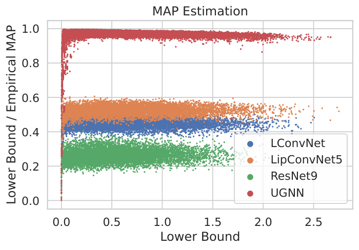
Figure 3 compares the ratio of the LB and the MAP between the -Lipschitz DDNs and a UGNN with MaxMin and bounded upd, for the normalized inputs. The MAP is computed with the expensive Iterative Penalty procedure, as done in (Brau et al. 2022). Note that our analysis considers the worst-case MAP, i.e., without box-constraints, as also done by the compared -Lipschitz models. Indeed, since image pixels are bounded in , the MAP is itself a lower bound of the distance from the closest adversarial image. Table 4 reports statistics related to the LB/MAP ratio for different UGNNs, where the box-constrained (B.C.) MAPs were computed using the Decoupling Direction Norm strategy (Rony et al. 2019). The column #N contains the number of samples correctly classified by the model and for which the MAP algorithm reached convergence. Note that, in all the tested cases, the LB provided by the UGNN resulted to be tighter than the other -Lipschitz DNNs. Similar considerations hold for other model configurations (see Appendix).
| Model | LB/MAP | #N | B.C |
|---|---|---|---|
| ResNet9 (raw) | 6669 | ✓ | |
| LargeConvNet (raw) | 7219 | ✓ | |
| LipConvNet5 (raw) | 6911 | ✓ | |
| UGNN+OPLU+updU (raw) | 7125 | ✓ | |
| UGNN+OPLU+updB (raw) | 7098 | ✓ | |
| UGNN+MaxMin+updB (raw) | 7114 | ✓ | |
| UGNN+MaxMin+updU (raw) | 7118 | ✓ | |
| ResNet9 (norm) | 7904 | ✗ | |
| LargeConvNet (norm) | 7933 | ✗ | |
| LipConvNet5 (norm) | 7840 | ✗ | |
| UGNN+OPLU+updB (norm) | 7215 | ✗ | |
| UGNN+OPLU+updU (norm) | 7282 | ✗ | |
| UGNN+MaxMin+updU (norm) | 7316 | ✗ | |
| UGNN+MaxMin+updB (norm) | 7327 | ✗ |
Certifiable Robust Classification
Figure 4 shows a close comparison of the accuracy of the (certifiable) -robust classifications for different values of , i.e., the percentage of correctly classified samples with a LB lower than .
We selected the UGNN with the highest accuracy (MaxMin-updB-256-raw). The tests for the 32x32 input size are provided in Appendix. The -Lipschitz models were trained on raw inputs, where the best run has been selected. For these models, to handle 256x256 images, an initial nearest interpolation from to is applied. This transformation is necessary since, differently from the UGNN, they are not adaptive to different input sizes. Note that the interpolation preserves both the accuracy and the -Lipschitz property. As shown in Fig. 4, the UGNN outperforms the other models for all the tested values.
Conclusion
This paper presented a novel family of classifiers, named Signed-Distance Classifiers (SDCs), which provides the minimal adversarial perturbation (MAP) by just computing the difference between the two highest output components, thus offering an online-certifiable prediction.
To practically implement an SDC, we developed a novel architecture, named Unitary-Gradient Neural Network (UGNN), which satisfies (almost-everywhere) the characterization property of an SDC. To design this model, we proposed a new fully-connected layer, named Unitary Pair Difference (UPD), which features unbounded weight matrix while preserving the unitary-gradient property.
Several experiments were conducted to compare the proposed architecture with the most related certifiable -Lipschitz models from previous work. The experiments highlighted the performance of the UGNN in terms of accuracy, certifiable robustness, and estimation of the MAP, showing promising results.
Future work will focus on improving the UGNN. Furthermore, as pointed out by other authors, additional investigations are needed to tackle practical open problems in this field, such as addressing dataset with many classes and improving learning strategies.
References
- Anil, Lucas, and Grosse (2019) Anil, C.; Lucas, J.; and Grosse, R. 2019. Sorting Out Lipschitz Function Approximation. In Proceedings of the 36th International Conference on Machine Learning, 291–301. PMLR.
- Biggio et al. (2013) Biggio, B.; Corona, I.; Maiorca, D.; Nelson, B.; Šrndić, N.; Laskov, P.; Giacinto, G.; and Roli, F. 2013. Evasion Attacks against Machine Learning at Test Time, volume 7908 of Lecture Notes in Computer Science, 387–402. Springer Berlin Heidelberg. ISBN 978-3-642-38708-1.
- Biggio and Roli (2018) Biggio, B.; and Roli, F. 2018. Wild Patterns: Ten Years After the Rise of Adversarial Machine Learning. In Proceedings of the 2018 ACM SIGSAC Conference on Computer and Communications Security, CCS ’18, 2154–2156. New York, NY, USA: Association for Computing Machinery. ISBN 9781450356930.
- Brau et al. (2022) Brau, F.; Rossolini, G.; Biondi, A.; and Buttazzo, G. 2022. On the Minimal Adversarial Perturbation for Deep Neural Networks With Provable Estimation Error. IEEE Transactions on Pattern Analysis and Machine Intelligence, 1–15.
- Béthune et al. (2021) Béthune, L.; González-Sanz, A.; Mamalet, F.; and Serrurier, M. 2021. The Many Faces of 1-Lipschitz Neural Networks. arXiv:2104.05097 [cs, stat]. ArXiv: 2104.05097.
- Carlini et al. (2018) Carlini, N.; Katz, G.; Barrett, C.; and Dill, D. L. 2018. Provably Minimally-Distorted Adversarial Examples. arXiv:1709.10207 [cs]. ArXiv: 1709.10207.
- Carlini and Wagner (2017) Carlini, N.; and Wagner, D. 2017. Towards Evaluating the Robustness of Neural Networks. In 2017 IEEE Symposium on Security and Privacy (SP), 39–57.
- Chernodub and Nowicki (2017) Chernodub, A.; and Nowicki, D. 2017. Norm-preserving Orthogonal Permutation Linear Unit Activation Functions (OPLU). arXiv:1604.02313.
- Cisse et al. (2017) Cisse, M.; Bojanowski, P.; Grave, E.; Dauphin, Y.; and Usunier, N. 2017. Parseval Networks: Improving Robustness to Adversarial Examples. arXiv:1704.08847 [cs, stat]. ArXiv: 1704.08847.
- Cohen, Rosenfeld, and Kolter (2019) Cohen, J.; Rosenfeld, E.; and Kolter, Z. 2019. Certified Adversarial Robustness via Randomized Smoothing. In Proceedings of the 36th International Conference on Machine Learning, 1310–1320. PMLR.
- Federer (1959) Federer, H. 1959. Curvature measures. Transactions of the American Mathematical Society, 93(3): 418–491.
- Goodfellow, Shlens, and Szegedy (2015) Goodfellow, I. J.; Shlens, J.; and Szegedy, C. 2015. Explaining and Harnessing Adversarial Examples. arXiv:1412.6572 [cs, stat]. ArXiv: 1412.6572.
- Hein and Andriushchenko (2017) Hein, M.; and Andriushchenko, M. 2017. Formal Guarantees on the Robustness of a Classifier against Adversarial Manipulation. In Advances in Neural Information Processing Systems, volume 30. Curran Associates, Inc.
- Kingma and Ba (2017) Kingma, D. P.; and Ba, J. 2017. Adam: A Method for Stochastic Optimization. arXiv:1412.6980.
- Lang (2012) Lang, S. 2012. Fundamentals of differential geometry, volume 191. Springer Science & Business Media.
- Li et al. (2019) Li, Q.; Haque, S.; Anil, C.; Lucas, J.; Grosse, R. B.; and Jacobsen, J.-H. 2019. Preventing Gradient Attenuation in Lipschitz Constrained Convolutional Networks. In Advances in Neural Information Processing Systems, volume 32. Curran Associates, Inc.
- Li et al. (2021) Li, S.; Jia, K.; Wen, Y.; Liu, T.; and Tao, D. 2021. Orthogonal Deep Neural Networks. IEEE Transactions on Pattern Analysis and Machine Intelligence, 43(4): 1352–1368.
- Liu and Nocedal (1989) Liu, D. C.; and Nocedal, J. 1989. On the limited memory BFGS method for large scale optimization. Mathematical programming, 45(1): 503–528.
- Madry et al. (2019) Madry, A.; Makelov, A.; Schmidt, L.; Tsipras, D.; and Vladu, A. 2019. Towards Deep Learning Models Resistant to Adversarial Attacks. (arXiv:1706.06083). ArXiv:1706.06083 [cs, stat].
- Miyato et al. (2018) Miyato, T.; Kataoka, T.; Koyama, M.; and Yoshida, Y. 2018. Spectral Normalization for Generative Adversarial Networks. arXiv:1802.05957 [cs, stat]. ArXiv: 1802.05957.
- Moosavi-Dezfooli, Fawzi, and Frossard (2016) Moosavi-Dezfooli, S.-M.; Fawzi, A.; and Frossard, P. 2016. DeepFool: A Simple and Accurate Method to Fool Deep Neural Networks. 2574–2582.
- Paszke et al. (2019) Paszke, A.; Gross, S.; Massa, F.; Lerer, A.; Bradbury, J.; Chanan, G.; Killeen, T.; Lin, Z.; Gimelshein, N.; Antiga, L.; Desmaison, A.; Kopf, A.; Yang, E.; DeVito, Z.; Raison, M.; Tejani, A.; Chilamkurthy, S.; Steiner, B.; Fang, L.; Bai, J.; and Chintala, S. 2019. PyTorch: An Imperative Style, High-Performance Deep Learning Library. In Advances in Neural Information Processing Systems 32, 8024–8035. Curran Associates, Inc.
- Pintor et al. (2021) Pintor, M.; Roli, F.; Brendel, W.; and Biggio, B. 2021. Fast minimum-norm adversarial attacks through adaptive norm constraints. Advances in Neural Information Processing Systems, 34: 20052–20062.
- Rony et al. (2020) Rony, J.; Granger, E.; Pedersoli, M.; and Ayed, I. B. 2020. Augmented Lagrangian Adversarial Attacks. arXiv:2011.11857 [cs]. ArXiv: 2011.11857.
- Rony et al. (2019) Rony, J.; Hafemann, L. G.; Oliveira, L. S.; Ayed, I. B.; Sabourin, R.; and Granger, E. 2019. Decoupling Direction and Norm for Efficient Gradient-Based L2 Adversarial Attacks and Defenses. arXiv:1811.09600 [cs]. ArXiv: 1811.09600.
- Rossolini, Biondi, and Buttazzo (2022) Rossolini, G.; Biondi, A.; and Buttazzo, G. 2022. Increasing the Confidence of Deep Neural Networks by Coverage Analysis. IEEE Transactions on Software Engineering.
- Sakai (1996) Sakai, T. 1996. On Riemannian manifolds admitting a function whose gradient is of constant norm. Kodai Mathematical Journal, 19(1).
- Schölkopf et al. (2002) Schölkopf, B.; Smola, A. J.; Bach, F.; et al. 2002. Learning with kernels: support vector machines, regularization, optimization, and beyond. MIT press.
- Serrurier et al. (2021) Serrurier, M.; Mamalet, F.; González-Sanz, A.; Boissin, T.; Loubes, J.-M.; and del Barrio, E. 2021. Achieving robustness in classification using optimal transport with hinge regularization. arXiv:2006.06520 [cs, stat]. ArXiv: 2006.06520.
- Shi et al. (2016) Shi, W.; Caballero, J.; Huszár, F.; Totz, J.; Aitken, A. P.; Bishop, R.; Rueckert, D.; and Wang, Z. 2016. Real-time single image and video super-resolution using an efficient sub-pixel convolutional neural network. In Proceedings of the IEEE conference on computer vision and pattern recognition, 1874–1883.
- Singla and Feizi (2021) Singla, S.; and Feizi, S. 2021. Skew Orthogonal Convolutions. In Proceedings of the 38th International Conference on Machine Learning, 9756–9766. PMLR.
- Singla, Singla, and Feizi (2021) Singla, S.; Singla, S.; and Feizi, S. 2021. Improved deterministic l2 robustness on CIFAR-10 and CIFAR-100. In International Conference on Learning Representations.
- Szegedy et al. (2013) Szegedy, C.; Zaremba, W.; Sutskever, I.; Bruna, J.; Erhan, D.; Goodfellow, I.; and Fergus, R. 2013. Intriguing properties of neural networks. arXiv preprint arXiv:1312.6199.
- Trockman and Kolter (2021) Trockman, A.; and Kolter, J. Z. 2021. Orthogonalizing Convolutional Layers with the Cayley Transform. arXiv:2104.07167 [cs, stat]. ArXiv: 2104.07167.
- Tsuzuku, Sato, and Sugiyama (2018) Tsuzuku, Y.; Sato, I.; and Sugiyama, M. 2018. Lipschitz-Margin Training: Scalable Certification of Perturbation Invariance for Deep Neural Networks. In Advances in Neural Information Processing Systems, volume 31. Curran Associates, Inc.
- Wang et al. (2020) Wang, J.; Chen, Y.; Chakraborty, R.; and Yu, S. X. 2020. Orthogonal Convolutional Neural Networks. In 2020 IEEE/CVF Conference on Computer Vision and Pattern Recognition (CVPR), 11502–11512. IEEE. ISBN 978-1-72817-168-5.
- Weng et al. (2018) Weng, T.-W.; Zhang, H.; Chen, P.-Y.; Yi, J.; Su, D.; Gao, Y.; Hsieh, C.-J.; and Daniel, L. 2018. Evaluating the Robustness of Neural Networks: An Extreme Value Theory Approach. arXiv:1801.10578 [cs, stat]. ArXiv: 1801.10578.
- Wong et al. (2018) Wong, E.; Schmidt, F. R.; Metzen, J. H.; and Kolter, J. Z. 2018. Scaling provable adversarial defenses. arXiv:1805.12514 [cs, math, stat]. ArXiv: 1805.12514.
Technical Appendix of “Robust-by-Design Classification via Unitary-Gradient Neural Networks”
Appendix A Gradient Norm Preserving
Activation Functions
Component-wise activation functions that satisfy Property GNP can be completely characterized; this is the aim of the following lemma.
Lemma 1 (GNP Component-wise Activation Functions).
The only component-wise activation functions that guarantee the orthogonal property GNP are the piecewise-linear functions with slope or .
Proof.
Let a scalar function, and let the tensor-wise version of defined as . Observe the corresponding Jacobian matrix is always represented by a diagonal matrix . The orthogonal condition on the Jacobian rows is only guaranteed if solves the differential equation
| (8) |
Observe that all the solutions of Equation 8 are of the form where , , and is a discrete partition of . Observe in conclusion that solves Equation 8. ∎
Tensor-wise GNP activation functions
The OPLU activation function was introduced in (Chernodub and Nowicki 2017) and recently generalized from (Anil, Lucas, and Grosse 2019). Accordingly with the original paper, we assume the following definition.
Definition 3 (OPLU).
The 2-dimensional version is defined as follows
| (9) | ||||
The generalization to higher dimensional spaces is the following
| (10) | ||||
Appendix B Characterization of the Signed Distance Functions
This section contains a proof of Theorem 1. For the sake of a clear comprehension, before providing the proof, let us remind some classical results. The following theorems are known as Existence and Uniqueness of Solutions of Ordinary Differential Equations (ODE) and Implicit Function Theorem.
Theorem 2 (Existence and Uniqueness of ODE solutions).
Let be an open subset of , and let a smooth function, i.e., , then the following statements hold.
- i)
For each and , there exists and open sets, with , such that for each there exists a solution of the following Cauchy-problem
(11) where we keep the notation to highlight that is the starting point of the solution of Problem 11.
- ii)
The map , namely flux, defined by , is in ;
- iii)
If are two solutions of Equation (11), then ;
Proof.
Refer to (Lang 2012, pp.66-88). ∎
The implicit function theorem can instead be stated as follows.
Theorem 3 (Implicit Function Theorem (Dini)).
Let be a smooth function defined on an open set . If is such that
then there exists an open set and a smooth function such that
| (12) |
Proof.
The proof can be deduced by (Lang 2012, Thm. 5.9), where , , and . ∎
Finally we can leverage these results to prove the main theorem of the paper.
Theorem 1 Let be an open set, and let be a function, smooth in , such that . If has a unitary gradient in , then there exists an open set such that coincides in with the signed distance function from . Formally,
| (13) |
Proof.
We have to prove that there exists an open set such that the unitary gradient property in implies that for all . The proof is divided in two main parts:
- (i)
Let us consider the following ordinary differential equation with initial condition (a.k.a. Cauchy problem)
(14) where . We show that there exists an open set such that each can be reached by a solution of the Cauchy-problem (14), i.e., such that for some ;
- (ii)
We show that any trajectory of the flux corresponds the minimal geodetic (i.e., the shortest path) between the hyper-surfaces of the form and . This can be obtained by explicitly deducing a close form of on .
Let us start with the existence of such a . Since is smooth, then satisfies the hypothesis of Theorem 2, by which we can deduce that for each there exists an open set such that the flux
| (15) | ||||
is of class (where remember that is the solution of the ODE (11) with starting point in ). Let be the smooth function defined by . By (14), and , hence it is possible to observe that
| (16) |
and that
| (17) |
We then deduce by the Implicit Function Theorem 3 that there exists an open set such that
| (18) |
from which
| (19) |
From the uniqueness of the solution stated in Theorem 2, this implies that, for each , there exists and an instant such that . Finally, by considering , the first step of the proof is concluded.
Now, we want to prove that the trajectory of the dynamic system coincides with the geodetic (the curve of minimal length) from any and for any . Let be the solution of (11) with starting point in , and let be the point of the trajectory for . Let us consider a function of the form to denote the curve that connects and . Observe that the length of can be found by considering the following formula
| (20) |
Since we can deduce that the length of is .
Let be any other curve that connects and . Observe that the following chain of inequalities holds
| (21) | ||||
where the first inequality is a direct consequence of the Cauchy-Schwarzt inequality ().
It remains to prove that . To do so, let us consider the following observation.
Observation 6.
If and , then .
Proof.
Let be the value of on the trajectory of the flux. Since we deduce . ∎
This concludes the second step of the proof, since for each curve that connects and we have that
hence is the shortest path between and , from which .
In conclusion, the theorem is proved by observing that, for each , there exists such that for some . Indeed, by the definition of , let such that , then there exists a such that for some . ∎
An example of non-affine Signed Distance Function
In the main paper, we observed that is an instance of a non-affine signed distance function. Indeed, observe that, for each , the gradient of has unitary euclidean norm and it has the following explicit formulation . Furthermore, the minimal adversarial perturbation problem relative to can be written as follows
| (22) |
and has a minimal solution of the form . This fact can be proved by considering the associated Lagrangian function , from which we can deduce that , is a stationary point of , i.e., there exists a Lagrangian multiplier such that , realized for .
Appendix C Extension to Multi Class Signed Classifiers
This section contains the technical details for the proof of Observation 2 related to the definition of the signed distance classifier for multi-class classification. Let us first consider the following lemma that shows that Problem MAP can be solved by considering the smallest solution of a sequence of a minimum problems
Lemma 2.
Let classified from with the class , . Let, for each , , then
where is the solution of the Problem 1 relative to the binary classifier . In formulas,
| (23) | |||||
Proof.
The main idea is to separately prove the two inequalities
| (24) |
The inequality on the right can be deduced by observing that, for each , the solution of the Problem 1, relative to the function , satisfies the constraints of the minimum problem MAP relative to the function . Hence, by the definition of minimum .
The inequality on the left is deduced by observing that if is the solution of and if is such that , then satisfies the constraints of the Problem 1 for the function . Hence,
which concludes the proof. ∎
Observation 2. Let a signed distance classifier and let a sample classified as , and let the second highest component. Then, the classifier
Proof.
The first statement is a direct consequence of Lemma 2. Consider the following chain of equalities
| (25) | ||||
where the second equivalence is given by the definition of a signed distance classifier. The second statement is a consequence of Observation 1, indeed, provides the direction of the shortest path to reach . ∎
Appendix D The PixelUnshuffle is a gradient norm preserving layer
Pixel-Unshuffle layer has a fundamental role in crafting a unitary gradient neural network, since it allows increasing the number of channels through the internal activations and, simultaneously, keeping the GNP property of the convolutions. A Pixel-Unshuffle layer, with scaling-size of , transforms an input only by rearranging its entries to provide an output tensor of shape . Such a layer, can be discribed as the inverse of the pixel-shuffle layer described as follows
where means the entry of the -th channel of the leftmost tensor. Hence, observe that the vectorized version of S can be described as a map such that , where and is a one-to-one permutation map. Finally observe that,
| (26) |
from which we can deduce that each row of the Jacobian contains one and only one not-zero entry (that is ), and, that every two rows are different. This very last statement directly implies the orthogonality of in each . In conclusion the GNP property of the pixel-unshuffle layer , can be deduced by observing that, if is the vectorized version of , then
Appendix E Parameterized Unitary Pair Difference Layer
This section aims at describing how the objective function can be efficiently computed by exploiting the parallelism. Let us consider the family of matrices , within rows and columns, recursively defined as follows
| (27) |
Hence, observe that if is some matrix, then the resulting matrix product corresponds to a matrix where each row is one of the possible difference between two rows of . In formulas
| (28) |
This allows exploiting the parallelism of the GPUs in order to efficiently compute the objective function .
In conclusion, experimental tests reported in Figure 5 show that iterations of the L-BFGS algorithm are sufficient to obtain a UPD matrix whose differences between rows have an euclidean norm in the range for the case of interest ().
Appendix F Unitary Gradient Neural Network
The Unitary Gradient Property
This section aims at empirically evaluating the euclidean norm of the pair difference to show that is numerically equal to . Distribution plots in Figure 6 show the distribution of the norm of the difference for a classifier with output classes.
Certifiable Robust Classification through UGNNs
This section aims at providing further details related to the robustness statements in Observation 5 reported below. Before going deeper in the details, it is worth to remind a known results.
Lemma 3.
Let a continuous function, differentiable almost-everywhere. If in each differentiable point , then is -Lipschitz.
Proof.
Let and be the straight line that connects the two points. Observe that, by the hypothesis, the function is continuous almost everywhere, from which
By applying the absolute value and considering the Cauchy–Schwarz inequality (), the following inequality holds
from which the thesis follows. ∎
Finally, the observation can be easily proved.
Observation 5 (Certifiable Robustness). If is a UGNN, then is robust in . In other words, is directly a lower bound of the MAP in .
Proof.
Let us assume such that is defined and such that . Let defined as follows
By the definition of UGNN, observe that , for each , hence, by Lemma 3, is -Lipschitz. By the definition of -Lipschitz functions, we deduce that, for each such that ,
where the first inequality is due to the lipschitz property and the second is due to the choose of . By considering only the negative part of the absolute value, we then obtain that
This implies that for all from which we can deduce that . In conclusion, let the minimal adversarial perturbation in , then since
then by considering the inferior on , we obtain that
which concludes the proof. ∎
Appendix G Supplementary Experimental Material
Further MAP Estimations Analysis
Table 5 and Figure 7 show the MAP estimation through the lower bound provided by the tested models for different cases.
| Model | LB/MAP | #N | B.C |
|---|---|---|---|
| ResNet9 (norm) | 7900 | ✓ | |
| ResNet9 (raw) | 6669 | ✓ | |
| LargeConvNet (norm) | 2148 | ✓ | |
| LipConvNet5 (norm) | 7838 | ✓ | |
| LargeConvNet (raw) | 7219 | ✓ | |
| LipConvNet5 (raw) | 6911 | ✓ | |
| UGNN+OPLU+updB (norm) | 7101 | ✓ | |
| UGNN+Abs+updB (norm) | 7220 | ✓ | |
| UGNN+OPLU+updU (norm) | 7281 | ✓ | |
| UGNN+Abs+updU (norm) | 7244 | ✓ | |
| UGNN+MaxMin+updU (norm) | 7311 | ✓ | |
| UGNN+MaxMin+updB (norm) | 4386 | ✓ | |
| UGNN+OPLU+updU (raw) | 7125 | ✓ | |
| UGNN+OPLU+updB (raw) | 7098 | ✓ | |
| UGNN+MaxMin+updB (raw) | 7114 | ✓ | |
| UGNN+MaxMin+updU (raw) | 7118 | ✓ | |
| UGNN+Abs+updB (raw) | 6960 | ✓ | |
| UGNN+Abs+updU (raw) | 6940 | ✓ | |
| ResNet9 (norm) | 7904 | ✗ | |
| ResNet9 (raw) | 6663 | ✗ | |
| LargeConvNet (norm) | 7933 | ✗ | |
| LipConvNet5 (norm) | 7840 | ✗ | |
| LargeConvNet (raw) | 2429 | ✗ | |
| LipConvNet5 (raw) | 6912 | ✗ | |
| UGNN+OPLU+updU (raw) | 6755 | ✗ | |
| UGNN+OPLU+updB (raw) | 7102 | ✗ | |
| UGNN+MaxMin+updU (raw) | 7127 | ✗ | |
| UGNN+MaxMin+updB (raw) | 7117 | ✗ | |
| UGNN+Abs+updB (raw) | 6965 | ✗ | |
| UGNN+Abs+updU (raw) | 6949 | ✗ | |
| UGNN+OPLU+updB (norm) | 7215 | ✗ | |
| UGNN+Abs+updB (norm) | 7228 | ✗ | |
| UGNN+OPLU+updU (norm) | 7282 | ✗ | |
| UGNN+MaxMin+updU (norm) | 7316 | ✗ | |
| UGNN+MaxMin+updB (norm) | 7327 | ✗ | |
| UGNN+Abs+updU (norm) | 7247 | ✗ |


The bar-plot in Figure 8 contains, for each value of , the ratio of samples for which the classification is not -robust according to the lower-bound, but that feature a minimal adversarial perturbation larger than . The higher the bar, the fewer the practically -robust classifications discarded as not robust due to a lose lower bound. Let assume the following definitions,
| (29) |
| (30) |
| (31) |
then, each bar of Figure 8 represents the value expressed by Equation (31).
Further Robustness Evaluation
As it can be observed from Figure 9, for the case of 32x32 inputs we noted the same relative drop of accuracy of the other -Lipschitz models proposed in previous work.