2020.

L. D. Abreu Address: Faculty of Mathematics
University of Vienna
Oskar-Morgenstern-Platz 1
1090 Vienna, Austria Email address: abreuluisdaniel@gmail.com Email address: michael.speckbacher@univie.ac.at , P. Balazs Address: Acoustics Research Institute
Austrian Academy of Sciences
Wohllebengasse 12-14, 1040 Vienna
Austria Email address: peter.balazs@oeaw.ac.at Email address: nicki.holighaus@oeaw.ac.at , N. Holighaus , F. Luef Address: Department of Mathematics, NTNU Trondheim, 7041 Trondheim, Norway Email address: franz.luef@ntnu.no and M. Speckbacher

Abstract.

We provide the foundations of a Hilbert space theory for the short-time Fourier transform (STFT) where the flat tori

\mathbb{T}_{N}^{2}=\mathbb{R}^{2}/(\mathbb{Z}\times N\mathbb{Z})=[0,1]\times[0,N]

act as phase spaces. We work on an $N$ -dimensional subspace $S_{N}$ of distributions periodic in time and frequency in the dual $S_{0}^{\prime}(\mathbb{R})$ of the Feichtinger algebra $S_{0}(\mathbb{R})$ and equip it with an inner product. To construct the Hilbert space $S_{N}$ we apply a suitable double periodization operator to $S_{0}(\mathbb{R})$ . On $S_{N}$ , the STFT is applied as the usual STFT defined on $S_{0}^{\prime}(\mathbb{R})$ . This STFT is a continuous extension of the finite discrete Gabor transform from the lattice onto the entire flat torus. As such, sampling theorems on flat tori lead to Gabor frames in finite dimensions. For Gaussian windows, one is lead to spaces of analytic functions and the construction allows to prove a necessary and sufficient Nyquist rate type result, which is the analogue, for Gabor frames in finite dimensions, of a well known result of Lyubarskii and Seip-Wallstén for Gabor frames with Gaussian windows and which, for $N$ odd, produces an explicit full spark Gabor frame. The compactness of the phase space, the finite dimension of the signal spaces and our sampling theorem offer practical advantages in some applications. We illustrate this by discussing a problem of current research interest: recovering signals from the zeros of their noisy spectrograms.

Key words and phrases:

short-time Fourier transform, flat torus, DGT frames, Feichtinger algebra, sampling theory

2010 Mathematics Subject Classification

42C40, 46E15, 42C30, 46E22, 42C15

1. Introduction

The short-time Fourier transform (STFT) is the central instrument of time-frequency analysis. The most classical setting considers the analysis of functions $f$ with respect to windows $g$ , both contained in $\mathrm{L}^{2}(\mathbb{R})$ , defined as

(1)

\mathbf{V}_{g}f(x,\xi)=\int_{\mathbb{R}}f(t)\overline{g(t-x)}e^{-2\pi i\xi t}dt=\left\langle f,\mathbf{M}_{\xi}\mathbf{T}_{x}g\right\rangle=\langle f,{\pi}(x,\xi)g\rangle,

where $\mathbf{T}_{x}f(t)=f(t-x)$ , $\mathbf{M}_{\xi}f(t)=e^{2\pi i\xi t}f(t)$ , and $\pi(x,\xi)=\mathbf{M}_{\xi}\mathbf{T}_{x}$ define the translation, modulation and time-frequency shift operators, respectively. By interpreting the brackets as a duality pairing, this definition also holds for pairs of test function and distribution spaces, like the Schwartz space and tempered distributions $\mathcal{S(\mathbb{R})},\mathcal{S}^{\prime}(\mathbb{R})$ [20] and, in particular, the Feichtinger algebra ${S}_{0}(\mathbb{R})$ and its dual ${S}_{0}^{\prime}(\mathbb{R})$ [14].

In this paper, we consider the STFT acting on the $N$ -dimensional space $S_{N}$ of time and frequency periodic distributions in ${S}^{\prime}_{0}(\mathbb{R})$ , see definitions in Section 2 and [19, Chapter 16.3] or [8, Chapter 6]. This will lead to new phase spaces for the joint time and frequency values: the flat tori $\mathbb{T}_{N}^{2}=[0,1]\times[0,N]$ , providing, as we will show, a continuous extension of the coefficient space of the discrete Gabor transform (DGT). The space $S_{N}$ is isometrically isomorphic to $\mathbb{C}^{N}$ equipped with the Euclidean norm and can similarly be obtained by sampling and periodization of $S_{0}(\mathbb{R})$ [24]. This connection implies that results for the STFT on $S_{N}$ have implications for the DGT on $\mathbb{C}^{N}$ and vice-versa. However, we will demonstrate that the STFT on the distribution space $S_{N}$ , embedded into ${S}^{\prime}_{0}(\mathbb{R})$ , has much stronger structural properties, similar to those enjoyed by the STFT on $\mathrm{L}^{2}(\mathbb{R})$ . As a continuous phase space extension of the DGT, the STFT on flat tori provides a natural way of defining off-the-grid values, offering flexibility in applications and the chance of using continuous variable methods in finite Gabor analysis.

In the case of Gaussian windows, we obtain spaces of analytic functions. The resulting possibility of using analytic complex variable tools will allow us to prove a necessary and sufficient Nyquist rate type result for Gabor frames with Gaussian windows in finite dimensions, which can be seen as the finite-dimensional analogue of the celebrated result of Seip-Wallstén [35] and Lyubarskii [28] for Gabor frames with Gaussian windows. The sufficient condition provides theoretical support to numerical procedures for increasing grid resolution, due to the principle of stable reconstruction using frames above the Nyquist rate. As a step in the proof of the sufficient Nyquist rate, we show that the STFT of any signal in $S_{N}$ with Gaussian window has exactly $N$ zeros, thereby making precise and proving the claim in [18]. This property of the toric STFT comes in handy for the problem of detecting noisy spectrogram zeros [6, 12, 10, 16]. The potential advantages of the toric setting for such applications will be further discussed in the final paragraph of the paper.

Our methods are innovative in the sense that they allow to obtain results for finite sequences merely as a byproduct of the theory on $S_{N}$ . But it must be noted that the relation between the continuous STFT and the discrete Gabor transform has been studied by several authors over the last 30 years, in particular by Janssen [23], and later by Kaiblinger [24] and Søndergaard [36, 37]. Where the works of Janssen and Søndergaard are concerned with the construction of discrete Gabor frames and dual windows from Gabor systems on $S_{0}(\mathbb{R})$ , Kaiblinger’s work is concerned with finite dimensional approximation of dual windows for Gabor frames on $S_{0}(\mathbb{R})$ . The sampling-periodization duality of the Fourier transform, succintly expressed in (generalizations of) Poisson’s summation formula and considered in many works, including [4, 9, 22, 24], is central to these contributions. In essence, the transition between $S_{0}(\mathbb{R})$ and $\mathbb{C}^{N}$ is achieved by studying a composition of periodization operators $\mathbf{P}_{(1)},\mathbf{P}_{(2)}$ on certain intervals with forward and inverse Fourier transforms $\mathcal{F}_{(1)},\mathcal{F}_{(2)}^{-1}$ as $\mathcal{F}_{(2)}^{-1}\mathbf{P}_{(2)}\mathcal{F}_{(1)}\mathbf{P}_{(1)}$ . Here, $\mathcal{F}_{(1)}$ is the Fourier transform of $\mathrm{L}^{2}(\mathbb{R})$ of a finite interval and $\mathcal{F}_{(2)}^{-1}$ is the inverse discrete Fourier transform. From this angle, the central deviation of the present paper from these prior works is that we consider $\mathcal{F}_{(1)}$ and $\mathcal{F}_{(2)}^{-1}$ to be distributional Fourier transforms on ${S}_{0}^{\prime}(\mathbb{R})$ , such that $\mathcal{F}_{(2)}^{-1}\mathbf{P}_{(2)}\mathcal{F}_{(1)}\mathbf{P}_{(1)}f$ , $f\in S_{0}(\mathbb{R})$ , yields a doubly periodic distribution in ${S}_{0}^{\prime}(\mathbb{R})$ instead of a finite sequence in $\mathbb{C}^{N}$ , enabling the subsequent application of the STFT on ${S}_{0}^{\prime}(\mathbb{R})$ instead of the DGT .

2. Overview

We consider functions, distributions, and finite sequences, denoted by lower case latin letters $f,g$ , greek letters $\phi,\psi$ , and sans font latin letters $\mathsf{f},\mathsf{g}$ , respectively. For the latter, the discrete nature of the domain of $\mathsf{f},\mathsf{g}$ is emphasized by using square brackets for indexing, e.g. $\mathsf{f}[l]$ . Operators are denoted by upper case letters $\mathbf{V},\mathbf{\Sigma}$ . Exceptions from this convention are time-frequency shifts $\pi$ , the Jacobi theta function $\vartheta$ , and the Fourier transform $\mathcal{F}$ , for which we adopt established notation.

With the Gaussian window $h_{0}(t)=e^{-\pi t^{2}}$ , the Feichtinger algebra ${S}_{0}(\mathbb{R})$ [13, 21] is the space

\begin{split}{S}_{0}(\mathbb{R})&:=\big\{f\in\mathrm{L}^{2}(\mathbb{R})\colon\mathbf{V}_{h_{0}}f\in\mathrm{L}^{1}(\mathbb{R}^{2})\big\},\ \text{equipped with the norm}\\ \|f\|_{{S}_{0}}&:=\int_{\mathbb{R}^{2}}|\mathbf{V}_{h_{0}}f(x,\xi)|dxd\xi=\|\mathbf{V}_{h_{0}}f\|_{\mathrm{L}^{1}(\mathbb{R}^{2})}.\end{split}

We define the space $S_{N}$ as the span of $\{\epsilon_{n}\}_{n=0}^{N-1}$ , the sequence of periodic delta trains [19]

(2)

\epsilon_{n}:=\sum_{k\in\mathbb{Z}}\delta_{\frac{n}{N}+k}\subset S_{0}^{\prime}(\mathbb{R}),\qquad n=0,...,N-1,

and will show that $S_{N}$ can be characterized as the image of $S_{0}(\mathbb{R})$ under the double periodization operator

(3)

\mathbf{\Sigma}_{N}f:=\sum_{k_{1},k_{2}\in\mathbb{Z}}\mathbf{M}_{Nk_{2}}\mathbf{T}_{k_{1}}f=\sum_{k_{1},k_{2}\in\mathbb{Z}}e^{2\pi iNk_{2}\,\bullet}\cdot f(\,\bullet-k_{1})\text{.}

It can be directly observed that $\mathbf{V}_{g}(\mathbf{\Sigma}_{N}f)$ is quasiperiodic, i.e.

(4)

\begin{array}[]{l}\mathbf{V}_{g}(\mathbf{\Sigma}_{N}f)(x+1,\xi)=e^{-2\pi i\xi}\mathbf{V}_{g}(\mathbf{\Sigma}_{N}f)(x,\xi),\\ \mathbf{V}_{g}(\mathbf{\Sigma}_{N}f)(x,\xi+N)=\mathbf{V}_{g}(\mathbf{\Sigma}_{N}f)(x,\xi).\end{array}

Thus, the phase spaces of $\mathbf{V}_{g}\circ\mathbf{\Sigma}_{N}$ are the flat tori $\mathbb{T}_{N}^{2}=[0,1]\times[0,N]$ . As we will see, $\mathbf{V}_{g}\circ\mathbf{\Sigma}_{N}:{S}_{0}(\mathbb{R})\rightarrow\mathrm{L}^{2}(\mathbb{T}_{N}^{2})$ and $\mathbf{V}_{g}:S_{N}\rightarrow\mathrm{L}^{2}(\mathbb{T}_{N}^{2})$ have the same range in phase-space. It will often be convenient to jump from one to the other representation to simplify proofs.

The STFT on $S_{N}$ naturally introduces the compact phase space $\mathbb{T}_{N}^{2}$ for time-frequency analysis on finite, $N$ -dimensional Hilbert spaces. Thereby, it provides a continuous model that, by construction, eliminates the truncation, or alternatively aliasing, errors usually associated with the transition from the STFT on $\mathrm{L}^{2}(\mathbb{R})$ to numerical implementations by means of the finite Gabor transform. That is not to say that these errors are removed: They are instead separated from the continuous model to the double periodization operator $\mathbf{\Sigma}_{N}$ , i.e., the mapping from ${S}_{0}(\mathbb{R})$ onto $S_{N}\subset{S}_{0}^{\prime}(\mathbb{R})$ .

As discussed in [23, 24, 37] in a slightly different formal framework, the composition $\mathbf{V}_{g}\circ\mathbf{\Sigma}_{N}$ relates to the discrete Gabor transform (DGT) on $\mathbb{C}^{N}$ , defined as

\mathbf{V}_{\mathsf{g}}\mathsf{f}\left[k,l\right]=\sum\limits_{m=0}^{N-1}\mathsf{f}[m]\overline{\mathsf{g}[m-k]}e^{\frac{-2\pi ilm}{N}},\quad\mathsf{f},\mathsf{g}\in\mathbb{C}^{N},

We will show that $\mathbf{V}_{g}$ maps $S_{N}$ into $\mathrm{L}^{2}(\mathbb{T}_{N}^{2})$ and that $\mathbf{V}_{g}$ can be viewed as a continuous extension of $\mathbf{V}_{\mathsf{g}}\colon\mathbb{C}^{N}\rightarrow\mathbb{C}^{N\times N}$ to $\mathbb{T}^{2}_{N}$ in the sense of the following result.

Theorem 1.

Let $f,g\in S_{0}(\mathbb{R})$ and let $\mathsf{f_{N}}=\mathbf{P}_{N}f,\mathsf{g_{N}}=\mathbf{P}_{N}g$ , with the periodization operator

\mathbf{P}_{N}\colon S_{0}(\mathbb{R})\rightarrow\mathbb{C}^{N},\quad\text{defined by}\quad f\mapsto\Big(\sum_{j\in\mathbb{Z}}f(n/N-j)\Big)_{n=0}^{N-1}.

Then, for $k,l\in 0,....,N-1$ ,

{\mathbf{V}}_{g}(\mathbf{\Sigma}_{N}f)\left(\frac{k}{N},l\right)=N^{-1}\cdot\mathbf{V}_{\mathsf{g_{N}}}\mathsf{f_{N}}[k,l].

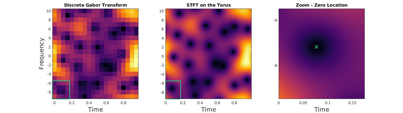
Specifically, the DGT can be obtained by sampling the phase space $\mathbb{T}^{2}_{N}$ of the continuous STFT restricted to $S_{N}$ on the grid points $(k/N,l)$ , providing a direct link between continuous and finite discrete time-frequency analysis. An example spectrogram of both the DGT and the STFT on the torus¹¹ 1 A MATLAB script reproducing Figure 1 can be downloaded from https://www.oeaw.ac.at/en/ari/torusSTFT. is shown in Figure 1.

Remark 2.

We chose the periods $(1,N)$ in Equation (3) for notational convenience. An arbitrary choice of $(c,d)\in\mathbb{R}^{2}_{+}$ and $(a,b)\in\mathbb{R}^{2}$ , with $cd=N$ , leads to equivalent results on the phase space $(a,b)\,+\,[0,c]\times[0,d]$ . When studying the approximation of the STFT by the DGT , as in [24], it is usually more convenient to consider the symmetric convention $(c,d)=(\sqrt{N},\sqrt{N})$ and $(a,b)=(-\sqrt{N}/2,-\sqrt{N}/2)$ , such that an increase in $N$ symmetrically expands the considered phase space $\tilde{\mathbb{T}}_{N}^{2}=[-\sqrt{N}/2,\sqrt{N}/2]\times[-\sqrt{N}/2,\sqrt{N}/2]$ and the sampling density within, covering all of $\mathbb{R}^{2}$ in the limit. The associated double periodization operator is independent of $(a,b)$ and given by $\tilde{\mathbf{\Sigma}}_{N}\colon f\mapsto\sum_{k_{1},k_{2}}e^{2\pi i\sqrt{N}k_{2}\,\bullet}\cdot f(\,\bullet\,-\sqrt{N}k_{1})$ .

Refer to caption — Figure 1. Comparison between the spectrograms obtained from the DGT and the STFT on the torus, and their application for detecting zeros of the STFT: Here, $\mathbf{P}_{N}f=\mathsf{f_{N}}$ was sampled from a complex Gaussian noise process $\mathcal{N}(0,I_{N})+i\mathcal{N}(0,I_{N})$ , $N=20$ . The right panel shows a zoom into the lower-left part of the spectrogram (indicated by the teal border), where the location of a spectrogram zero is marked.

We will study the Hilbert space properties of the map

\mathbf{V}_{g}:S_{N}\rightarrow\mathrm{L}^{2}(\mathbb{T}_{N}^{2})\text{,}

and derive the Moyal-type orthogonality relation

\int_{\mathbb{T}_{N}^{2}}\mathbf{V}_{g_{1}}\varphi_{1}(x,\xi)\overline{\mathbf{V}_{g_{2}}\varphi_{2}(x,\xi)}dxd\xi=N\langle\varphi_{1},\varphi_{2}\rangle_{S_{N}}\langle g_{2},g_{1}\rangle_{\mathrm{L}^{2}},

as well as inversion and reproducing formulas similar to those of the continuous STFT.

For the STFT with dilated Gaussian windows $h_{0}^{\lambda}(t)=e^{-\pi\lambda t^{2}}$ we will obtain a sampling theorem on the torus which leads to a full description of the frame set for finite Gabor frames with Gaussian windows in $\mathbb{C}^{N}$ . The proof uses a Bargmann-type transform, (which up to a weight is the STFT with $h_{0}^{\lambda}$ ) whose action on the space $S_{N}$ has previously been considered in a slightly different form in [27]. Finally, combining the sampling theorem on the torus with Theorem 1, we are lead to the following full description of the frame set for finite Gabor expansions using a periodized, dilated Gaussian window. As far as we could check, this is a completely new result.

Theorem 3.

Let $\lambda>0$ , $\mathsf{h_{N}^{\lambda}}=\mathbf{P}_{N}h_{0}^{\lambda}$ , and $\{(j_{k},l_{k})\}_{k=1,...,K}$ be a collection of distinct pairs of integers $j_{k},l_{k}\in 0,....,N-1$ . The following are equivalent:

1).

The set $\{(j_{k},l_{k})\}_{k=1,...,K}$ gives rise to a finite Gabor frame with window $\mathsf{h_{N}^{\lambda}}$ , i.e., there are constants $A,B>0$ such that, for every $\mathbf{f}\in\mathbb{C}^{N}$ ,

A\left\|\mathsf{f}\right\|_{\mathbb{C}^{N}}^{2}\leq\sum_{k=1}^{K}\left|\mathbf{V}_{\mathsf{h_{N}^{\lambda}}}\mathsf{f}[j_{k},l_{k}]\right|^{2}\leq B\left\|\mathsf{f}\right\|_{\mathbb{C}^{N}}^{2}\text{.}

2).
One of the three following conditions is satisfied:
1. (i)
  
  $N^{2}\geq K\geq N+1,$
2. (ii)
  
  $K=N$ is odd,
3. (iii)
  
  $K=N$ is even and $\sum_{k=1}^{N}(j_{k},l_{k})\notin N\mathbb{N}\times N\mathbb{N}.$

We emphasize that this result has been possible to prove only thanks to our Hilbert space theory for the STFT on flat tori, and that it strongly depends on the use of complex variable methods for quasi periodic analytic functions. This reinforces the suggestion that time-frequency analysis on the torus provides a rich theory which encompasses the theory of finite Gabor frames and leads to new insights, potential in applications and proof of results which were out of reach without the toric phase space.

The paper is organized as follows. Some required properties of the Hilbert space $S_{N}$ and the operator $\mathbf{\Sigma}_{N}$ are presented in Section 3. Section 4 contains the proof of Theorem 1 above, explicit computations with dilated Gaussian windows $h_{0}^{\lambda}$ , and derivations of the Moyal-type formula, together with the inversion and reproducing kernel formulas. In the last section, the window is specialized to be the Gaussian. The resulting Bargmann-type transform is defined, and several properties of its range space of entire functions with periodic constraints (a toric analogue of the Fock space) are studied in detail. All these properties are then used in the proof of the main result of the section: the sampling theorem on the torus. Finally, combining this result with Theorem 1, we derive a full characterization of finite Gabor frames with periodized and sampled Gaussian windows.

3. Properties of $S_{N}$ and $\mathbf{\Sigma}_{N}$

3.1. The Hilbert space $S_{N}$ of time-frequency periodic distributions

The space $S_{N}$ appears in theoretical physics in coherent state approaches [8, 19]. By definition of $S_{N}$ it is clear that the family $\{\epsilon_{n}\}_{n=0}^{N-1}$ defined in (2) forms a basis. Therefore, expanding $\varphi,\psi\in S_{N}$ with respect to this basis

\varphi=\sum_{n=0}^{N-1}a_{n}\epsilon_{n},\qquad\psi=\sum_{n=0}^{N-1}b_{n}\epsilon_{n},

we can define an inner product on $S_{N}$ by

\left\langle\varphi,\psi\right\rangle_{S_{N}}=\sum_{n=0}^{N-1}a_{n}\overline{b_{n}}.

Clearly, $S_{N}$ can be identified with $\mathbb{C}^{N}$ equipped with the standard inner product, and $\{\epsilon_{n}\}_{n=0}^{N-1}$ forms an orthonormal basis of $S_{N}$ as

\left\langle\epsilon_{n},\epsilon_{m}\right\rangle_{S_{N}}=\delta_{n,m}\text{.}

Note that for every $\varphi\in S_{N}$

(5)

\mathbf{T}_{1}\varphi=\varphi,\quad\text{ and }\quad\mathbf{M}_{N}\varphi=\varphi.

Therefore, $S_{N}$ is a space of distributions that are periodic in time and frequency. Actually, $S_{N}$ contains all distributions in $S_{0}^{\prime}(\mathbb{R})$ that satisfy (5), see [19, page 262, (16.12)].

3.2. The double periodization operator $\mathbf{\Sigma}_{N}$

We formally define the double periodization operator as

f\mapsto\mathbf{\Sigma}_{N}f=\sum_{k_{1},k_{2}\in\mathbb{Z}}\mathbf{M}_{Nk_{2}}\mathbf{T}_{k_{1}}f.

The next lemma shows when and in which sense this object is well-defined.

Lemma 4.

The operator $\mathbf{\Sigma}_{N}$ is well-defined from ${S}_{0}(\mathbb{R})$ into ${S}_{0}^{\prime}(\mathbb{R})$ with unconditional weak- $\ast$ convergence in ${S}_{0}^{\prime}(\mathbb{R})$ .

Proof: If $f,g\in{S}_{0}(\mathbb{R})$ , then

	$\displaystyle\|\mathbf{V}_{g}(\mathbf{\Sigma}_{N}f)(x,\xi)\|$	$\displaystyle\leq\sum_{k_{1},k_{2}\in\mathbb{Z}}\|e^{-2\pi ik_{1}\xi}\mathbf{V}_{g}f(x-k_{1},\xi-Nk_{2})\|$
		$\displaystyle\leq\sum_{k_{1},k_{2}\in\mathbb{Z}}\|\mathbf{V}_{g}(\mathbf{T}_{-x}\mathbf{M}_{-\xi}f)(k_{1},Nk_{2})\|$
		$\displaystyle\leq C\\|\mathbf{T}_{-x}\mathbf{M}_{-\xi}f\\|_{S_{0}}\\|g\\|_{S_{0}}$
		$\displaystyle\leq C\\|f\\|_{S_{0}}\\|g\\|_{S_{0}}\leq\infty,$

by [20, Lemma 3.1.3 and Corollary 12.1.12]. This implies that $\mathbf{\Sigma}_{N}f\in{S}_{0}^{\prime}(\mathbb{R})$ is well-defined. If we choose $x=\xi=0$ , then absolute weak- $\ast$ convergence of the series $\mathbf{\Sigma}_{N}f$ in $S_{0}^{\prime}(\mathbb{R})$ follows which in turn implies unconditional convergence. $\Box$

Remark 5.

It is easy to see that

0<\|\mathbf{V}_{g}(\mathbf{\Sigma}_{N}f)-\mathbf{V}_{g}f|_{\mathbb{T}^{2}_{N}}\|_{\mathrm{L}^{1}(\mathbb{T}^{2}_{N})}\leq\|(1-\mathds{1}_{\mathbb{T}^{2}_{N}})\mathbf{V}_{g}f\|_{\mathrm{L}^{1}(\mathbb{R}^{2})},

for all $0\neq f\in S_{0}(\mathbb{R})$ . That is, the double periodization introduces a nonzero, but controllable distortion in the STFT. Using the alternative phase space and double periodization convention introduced in Remark 2, we obtain the analogous statement $0<\|\mathbf{V}_{g}(\tilde{\mathbf{\Sigma}}_{N}f)-\mathbf{V}_{g}f|_{\tilde{\mathbb{T}}^{2}_{N}}\|_{\mathrm{L}^{1}(\tilde{\mathbb{T}}^{2}_{N})}\leq\|(1-\mathds{1}_{\tilde{\mathbb{T}}^{2}_{N}})\mathbf{V}_{g}f\|_{\mathrm{L}^{1}(\mathbb{R}^{2})}$ , where

\|(1-\mathds{1}_{\tilde{\mathbb{T}}^{2}_{N}})\mathbf{V}_{g}f\|_{\mathrm{L}^{1}(\mathbb{R}^{2})}\overset{N\rightarrow\infty}{\longrightarrow}0,

i.e., the distortion can be made arbitrarily small by increasing $N$ . If $f$ is even in a weighted $\mathrm{L}^{1}$ -type modulation space, i.e., $\omega\cdot\mathbf{V}_{g}f\in\mathrm{L}^{1}(\mathbb{R}^{2})$ for some weight function $\omega\colon\mathbb{R}^{2}\rightarrow[1,\infty)$ , then we can quantify the rate of convergence. Using the equality $\mathbf{V}_{g}f(x,\xi)=\mathbf{V}_{\mathbf{D}g}\mathbf{D}f(\sqrt{N}x,\xi/\sqrt{N})$ , where $\mathbf{D}=\mathbf{D}_{\sqrt{N}}$ denotes the unitary dilation $\mathbf{D}_{\sqrt{N}}\colon f\mapsto N^{1/4}f(\sqrt{N}\,\bullet\,)$ , we can derive a similar, but slightly less intuitive, statement on $\mathbb{T}^{2}_{N}$ .

As $\mathbf{\Sigma}_{N}f$ is periodic in time and frequency, we can expand it with respect to the orthonormal basis $\left\{\epsilon_{n}\right\}_{n=0}^{N-1}$ . In the next lemma, this expansion is obtained explicitly. We will also show that $\mathbf{\Sigma}_{N}$ is surjective as a mapping from $S_{0}(\mathbb{R})$ to $S_{N}$ . To do so, we need to define the periodization operator $\mathbf{P}f(t)=\sum_{k\in\mathbb{Z}}f(t-k)$ .

Lemma 6.

For every $f\in{S}_{0}(\mathbb{R})$

(6)

\mathbf{\Sigma}_{N}f=\frac{1}{N}\mathbf{P}f\cdot\sum_{k\in\mathbb{Z}}\delta_{\frac{k}{N}}=\frac{1}{N}\sum_{n=0}^{N-1}\mathbf{P}f\left(\frac{n}{N}\right)\epsilon_{n}\in S_{N}\text{,}

and

(7)

\langle\mathbf{\Sigma}_{N}f,g\rangle_{{S}_{0}^{\prime}\times{S}_{0}}=\frac{1}{N}\sum_{n=0}^{N-1}\mathbf{P}f\left(\frac{n}{N}\right)\overline{\mathbf{P}g\left(\frac{n}{N}\right)}=N\cdot\langle\mathbf{\Sigma}_{N}f,\mathbf{\Sigma}_{N}g\rangle_{S_{N}}\text{.}

Moreover, $\mathbf{\Sigma}_{N}:{S}_{0}(\mathbb{R})\rightarrow S_{N}$ is surjective.

Proof: Let $f,g\in{S}_{0}(\mathbb{R})$ . Since the Poisson summation formula holds for functions in ${S}_{0}(\mathbb{R})$ (see e.g. [20, Corollary 12.1.5]), we have that the following equality holds in the distributional sense

\sum_{k\in\mathbb{Z}}e^{2\pi iktN}=\frac{1}{N}\sum_{k\in\mathbb{Z}}\delta_{\frac{k}{N}}(t)\in S_{N}.

This shows that

\mathbf{\Sigma}_{N}f=\sum_{k\in\mathbb{Z}}\mathbf{M}_{Nk}\sum_{l\in\mathbb{Z}}\mathbf{T}_{l}f=\sum_{k\in\mathbb{Z}}\mathbf{M}_{Nk}\mathbf{P}f=\frac{1}{N}\sum_{k\in\mathbb{Z}}\delta_{\frac{k}{N}}\mathbf{P}f

with unconditional weak- $\ast$ convergence in ${S}_{0}^{\prime}(\mathbb{R})$ . Hence,

\langle\mathbf{\Sigma}_{N}f,g\rangle_{{S}_{0}^{\prime}\times{S}_{0}}=\frac{1}{N}\left\langle\sum_{k\in\mathbb{Z}}\delta_{\frac{k}{N}}\mathbf{P}f,g\right\rangle_{{S}_{0}^{\prime}\times{S}_{0}}.

Let us write

\sum_{k\in\mathbb{Z}}\delta_{\frac{k}{N}}=\sum_{n=0}^{N-1}\sum_{k\in\mathbb{Z}}\delta_{\frac{n}{N}+k}=\sum_{n=0}^{N-1}\epsilon_{n}

where the change of summation order is justified by e.g. [20, Corollary 12.1.5]. Using the periodicity of $\mathbf{P}f$ then yields

	$\displaystyle\langle\mathbf{\Sigma}_{N}f,g\rangle_{{S}_{0}^{\prime}\times{S}_{0}}$	$\displaystyle=\frac{1}{N}\sum_{n=0}^{N-1}\left\langle\sum_{k\in\mathbb{Z}}\delta_{\frac{n}{N}+k}\mathbf{P}f,g\right\rangle_{{S}_{0}^{\prime}\times{S}_{0}}$
		$\displaystyle=\frac{1}{N}\sum_{n=0}^{N-1}\sum_{k\in\mathbb{Z}}\mathbf{P}f\left(\frac{n}{N}+k\right)\overline{g\left(\frac{n}{N}+k\right)}$
		$\displaystyle=\frac{1}{N}\sum_{n=0}^{N-1}\mathbf{P}f\left(\frac{n}{N}\right)\sum_{k\in\mathbb{Z}}\overline{g\left(\frac{n}{N}+k\right)}$
		$\displaystyle=\frac{1}{N}\sum_{n=0}^{N-1}\mathbf{P}f\left(\frac{n}{N}\right)\langle\epsilon_{n},g\rangle_{{S}_{0}^{\prime}\times{S}_{0}}.$

Hence, (6) holds. The first equality of (7) follows from the second to last equality above. Finally, the second equality of (7) results from combining (6) and the first equality of (7).

It thus remains to show that $\mathbf{\Sigma}_{n}:{S}_{0}(\mathbb{R})\rightarrow S_{N}$ is surjective. By (6) it suffices to show that there exists a family of function $f_{n}\in{S}_{0}(\mathbb{R})$ , $n=0,\ldots,N-1$ , satisfying $\mathbf{P}f_{n}\left(\frac{k}{N}\right)=\delta_{n}(k),$ $k=0,\ldots,N-1$ . Such functions obviously exists. Take for instance $f_{n}(t):=\sinc(Nt-n)\cdot e^{-\pi(t-n/N)^{2}}$ which is even a Schwartz function. $\Box$

4. Time-frequency analysis on flat tori

4.1. Basic properties of $\mathbf{V}_{g}$ on $S_{N}$

The STFT defined on $S_{N}$ is, as we we subsequently show, closely connected to the Zak transform which is defined as

\mathbf{Z}f(x,\xi)=\sum_{k\in\mathbb{Z}}f(x-k)e^{2\pi ik\xi}.

For later reference we state here some elementary facts about the Zak transform (see e.g. [20]):

Quasiperiodicity:

(8)

\mathbf{Z}f(x,\xi+k)=\mathbf{Z}f(x,\xi),\quad\text{and}\quad\mathbf{Z}f(x+k,\xi)=e^{2\pi ik\xi}\mathbf{Z}(x,\xi),\quad k\in\mathbb{Z},

Action on time-frequency shifts:

(9)

\mathbf{Z}(\mathbf{M}_{\omega}\mathbf{T}_{y}f)(x,\xi)=e^{2\pi i\omega x}\mathbf{Z}f(x-y,\xi-\omega),

Unitarity: for $f_{1},f_{2}\in\mathrm{L}^{2}(\mathbb{R})$ it holds

(10)

\int_{0}^{1}\int_{0}^{1}\mathbf{Z}f_{1}(x,\xi)\overline{\mathbf{Z}f_{2}(x,\xi)}dxd\xi=\langle f_{1},f_{2}\rangle_{\mathrm{L}^{2}}.

The following lemma shows that $\mathbf{V}_{g}$ can be easily computed as a linear combination of shifted Zak transforms of the window $g$ .

Lemma 7.

Let $f,g\in{S}_{0}(\mathbb{R})$ and $\varphi\in S_{N}$ . Then

(11)

\mathbf{V}_{g}(\mathbf{\Sigma}_{N}f)(x,\xi)=\sum_{n=0}^{N-1}\mathbf{P}f\left(\frac{n}{N}\right)e^{-2\pi i\xi\frac{n}{N}}\mathbf{Z}\overline{g}\left(\frac{n}{N}-x,\xi\right),

and for $\varphi=\sum_{n=1}^{N}a_{n}\epsilon_{n}$

(12)

\mathbf{V}_{g}\varphi(x,\xi)=\sum_{n=0}^{N-1}a_{n}e^{-2\pi i\xi\frac{n}{N}}\mathbf{Z}\overline{g}\left(\frac{n}{N}-x,\xi\right).

Proof: First, let us compute the STFT of the basis functions $\epsilon_{n}$

	$\displaystyle\mathbf{V}_{g}\epsilon_{n}(x,\xi)$	$\displaystyle=\left\langle\epsilon_{n},\mathbf{M}_{\xi}\mathbf{T}_{x}g\right\rangle_{\mathcal{S}_{0}^{\prime}\times\mathcal{S}_{0}}=\sum_{k\in\mathbb{Z}}\left\langle\delta_{\frac{n}{N}+k},\mathbf{M}_{\xi}\mathbf{T}_{x}g\right\rangle_{\mathcal{S}_{0}^{\prime}\times\mathcal{S}_{0}}$
(13)			$\displaystyle=\sum_{k\in\mathbb{Z}}\overline{g\left(\frac{n}{N}+k-x\right)}e^{-2\pi i\xi(\frac{n}{N}+k)}=e^{-2\pi i\xi\frac{n}{N}}\mathbf{Z}\overline{g}\left(\frac{n}{N}-x,\xi\right),$

For general $\varphi=\sum_{n=0}^{N-1}a_{n}\epsilon_{n}\in S_{N}$ one thus gets (12). Applying $\mathbf{V}_{g}$ to (6) from Lemma 6 gives

\mathbf{V}_{g}(\Sigma_{N}f)(x,\xi)=\frac{1}{N}\sum_{n=0}^{N-1}\mathbf{P}f\left(\frac{n}{N}\right)\mathbf{V}_{g}\epsilon_{n}(x,\xi)

which combined with (13) yields (11). $\Box$

With these basic observations, it is now straightforward to show Theorem 1. For convenience, we repeat the statement here.

Theorem 1.

Let $f,g\in S_{0}(\mathbb{R})$ and let $\mathsf{f_{N}}=\mathbf{P}_{N}f,\mathsf{g_{N}}=\mathbf{P}_{N}g$ . Then, for $l,k\in 0,....,N-1$ ,

\mathbf{V}_{g}(\mathbf{\Sigma}_{N}f)\left(\frac{k}{N},l\right)=N^{-1}\cdot\mathbf{V}_{\mathsf{g_{N}}}\mathsf{f_{N}}[k,l].

Proof: Setting $\xi=l\in 0,....,N-1$ and $x=\frac{k}{N},\ k\in 0,\ldots,N-1,$ yields

	$\displaystyle\mathbf{V}_{g}(\mathbf{\Sigma}_{N}f)\left(\frac{k}{N},l\right)$	$\displaystyle=\frac{1}{N}\sum_{n=0}^{N-1}\mathbf{P}f\left(\frac{n}{N}\right)e^{-2\pi i\frac{nl}{N}}\mathbf{Z}\overline{g}\left(\frac{n-k}{N},l\right)$
		$\displaystyle=\frac{1}{N}\sum_{n=0}^{N-1}\mathbf{P}f\left(\frac{n}{N}\right)e^{-2\pi i\frac{nl}{N}}\overline{\mathbf{P}g}\left(\frac{n-k}{N}\right)$

This shows that by definition of the DGT we get the equality

\mathbf{V}_{g}(\mathbf{\Sigma}_{N}f)\left(\frac{k}{N},l\right)=\frac{1}{N}\mathbf{V}_{\mathsf{g_{N}}}\mathsf{f_{N}}[k,l].

$\Box$

Remark 8.

In fact, we can express $\mathbf{V}_{g}\varphi(x,\xi)$ , with $\varphi=\sum_{n=1}^{N}a_{n}\epsilon_{n}$ , in terms of the DGT for arbitrary $(x,\xi)\in\mathbb{T}^{2}_{N}$ . Since the expression in Eq. (12) relies on the $\mathbf{L}^{2}(\mathbb{R})$ -Zak transform, doing so may be more convenient for implementations. Specifically, with $\mathrm{f_{N}}=(a_{1},\ldots,a_{N})^{T}\in\mathbb{C}^{N}$ , we have

(14)

\mathbf{V}_{g}\varphi(x,\xi)=\exp(-2\pi ir_{\xi}n_{x}/N)\cdot\mathbf{V}_{\mathrm{g}^{(r_{x},r_{\xi})}_{\mathrm{N}}}\mathrm{f_{N}}[n_{x},m_{\xi}],

where $x=n_{x}/N+r_{x}$ and, $\xi=m_{\xi}+r_{\xi}$ , with $r_{x}\in[0,1/N)$ , $r_{\xi}\in[0,1)$ , and

\mathrm{g}_{\mathrm{N}}^{(r_{x},r_{\xi})}=\mathbf{P}_{N}(\mathbf{M}_{r_{\xi}}\mathbf{T}_{r_{x}}g).

To show this, begin by inserting the definition of $\mathbf{Z}\overline{g}$ in Eq. (12) to obtain

\begin{split}\mathbf{V}_{g}\varphi(x,\xi)&=\sum_{n=0}^{N-1}a_{n}e^{-2\pi i\xi\frac{n}{N}}\cdot\sum_{k\in\mathbb{Z}}\overline{g}(n/N-x-k)e^{2\pi ik\xi}\\ &=\sum_{n=0}^{N-1}a_{n}e^{-2\pi im_{\xi}\frac{n}{N}}\cdot\sum_{k\in\mathbb{Z}}\overline{g}\left(\frac{n-n_{x}}{N}-k-r_{x}\right)e^{-2\pi i(\frac{n}{N}-k)r_{\xi}}.\end{split}

Now, note that

\begin{split}\lx@add@cssclass{ltx_eqn_lefteqn}$\displaystyle\sum_{k\in\mathbb{Z}}\overline{g}\left(\frac{n-n_{x}}{N}-k-r_{x}\right)e^{-2\pi i(\frac{n}{N}-k)r_{\xi}}$\mbox{}\hfil\\ &=e^{-2\pi ir_{\xi}\frac{n_{x}}{N}}\cdot\overline{\left(\sum_{k\in\mathbb{Z}}g(\,\bullet\,-k-r_{x})e^{2\pi i(\,\bullet\,-k)r_{\xi}}\right)}\left(\frac{n-n_{x}}{N}\right)\\ &=e^{-2\pi ir_{\xi}\frac{n_{x}}{N}}\cdot\overline{\mathbf{P}_{N}(\mathbf{M}_{r_{\xi}}\mathbf{T}_{r_{x}}g)}[n-n_{x}]=e^{-2\pi ir_{\xi}\frac{n_{x}}{N}}\cdot\overline{\mathrm{g}_{\mathrm{N}}^{(r_{x},r_{\xi})}}[n-n_{x}].\end{split}

Together, we have

\mathbf{V}_{g}\varphi(x,\xi)=e^{-2\pi ir_{\xi}\frac{n_{x}}{N}}\sum_{n=0}^{N-1}a_{n}e^{-2\pi im_{\xi}\frac{n}{N}}\cdot\overline{\mathrm{g}_{\mathrm{N}}^{(r_{x},r_{\xi})}}[n-n_{x}],

proving (14), since $\mathrm{f_{N}}[n]=a_{n}$ .

4.2. Moyal-type and inversion formulas for the STFT on flat tori

One of the most fundamental identities in time-frequency analysis is Moyal’s formula ensuring that the STFT is an isometry from $\mathrm{L}^{2}(\mathbb{R})$ to $\mathrm{L}^{2}(\mathbb{R}^{2})$

\int_{\mathbb{R}^{2}}\mathbf{V}_{g_{1}}f_{1}(x,\xi)\overline{\mathbf{V}_{g_{2}}f_{2}(x,\xi)}dxd\xi=\langle f_{1},f_{2}\rangle_{\mathrm{L}^{2}}\langle g_{2},g_{1}\rangle_{\mathrm{L}^{2}},\quad f_{1},f_{2},g_{1},g_{2}\in\mathrm{L}^{2}(\mathbb{R}).

We will now show the toric equivalent of this identity ensuring that the STFT on the flat tori is a multiple of an isometry.

Theorem 9.

If $\varphi_{1},\varphi_{2}\in S_{N}$ , and $g_{1},g_{2}\in{S}_{0}(\mathbb{R})$ , then

(15)

\int_{\mathbb{T}_{N}^{2}}\mathbf{V}_{g_{1}}\varphi_{1}(x,\xi)\overline{\mathbf{V}_{g_{2}}\varphi_{2}(x,\xi)}dxd\xi=N\langle\varphi_{1},\varphi_{2}\rangle_{S_{N}}\langle g_{2},g_{1}\rangle_{\mathrm{L}^{2}}.

Proof: For $\varphi_{1}=\sum_{n=0}^{N-1}a_{n}\epsilon_{n}$ , and $\varphi_{2}=\sum_{n=0}^{N-1}b_{n}\epsilon_{n}$ , we use Lemma 7 and the periodicity of the Zak transform in the frequency variable (8) to obtain

	$\displaystyle\int_{\mathbb{T}_{N}^{2}}\mathbf{V}_{g_{1}}\varphi_{1}$	$\displaystyle(x,\xi)\overline{\mathbf{V}_{g_{2}}\varphi_{2}(x,\xi)}dxd\xi$
		$\displaystyle=\int_{0}^{N}\int_{0}^{1}\sum_{n,k=0}^{N-1}a_{n}\overline{b_{k}}e^{-2\pi i\xi\frac{n-k}{N}}\mathbf{Z}\overline{g_{1}}\left(\frac{n}{N}-x,\xi\right)\overline{\mathbf{Z}\overline{g_{2}}\left(\frac{k}{N}-x,\xi\right)}dxd\xi$
		$\displaystyle=\sum_{l=0}^{N-1}\int_{0}^{1}\int_{0}^{1}\sum_{n,k=0}^{N-1}a_{n}\overline{b_{k}}e^{-2\pi i(\xi+l)\frac{n-k}{N}}\cdot$
		$\displaystyle\hskip 95.0pt\mathbf{Z}\overline{g_{1}}\left(\frac{n}{N}-x,\xi+l\right)\overline{\mathbf{Z}\overline{g_{2}}\left(\frac{k}{N}-x,\xi+l\right)}dxd\xi$
		$\displaystyle=\int_{0}^{1}\int_{0}^{1}\sum_{n,k=0}^{N-1}a_{n}\overline{b_{k}}\left(\sum_{l=0}^{N-1}e^{-2\pi il\frac{n-k}{N}}\right)e^{-2\pi i\xi\frac{n-k}{N}}\cdot$
		$\displaystyle\hskip 95.0pt\mathbf{Z}\overline{g_{1}}\left(\frac{n}{N}-x,\xi\right)\overline{\mathbf{Z}\overline{g_{2}}\left(\frac{k}{N}-x,\xi\right)}dxd\xi$
		$\displaystyle=N\sum_{n=0}^{N-1}a_{n}\overline{b_{n}}\int_{0}^{1}\int_{0}^{1}\mathbf{Z}\overline{g_{1}}\left(\frac{n}{N}-x,\xi\right)\overline{\mathbf{Z}\overline{g_{2}}\left(\frac{n}{N}-x,\xi\right)}dxd\xi,$

where we used the basic fact $\sum_{l=0}^{N-1}e^{-2\pi il\frac{k}{N}}=N\delta_{k,0}$ , for $k=0,\dots,N-1$ , to obtain the final equality. Applying consecutively (9), (8) and (10) to the integral above yields

	$\displaystyle\int_{0}^{1}\int_{0}^{1}$	$\displaystyle\mathbf{Z}\overline{g_{1}}\left(\frac{n}{N}-x,\xi\right)\overline{\mathbf{Z}\overline{g_{2}}\left(\frac{n}{N}-x,\xi\right)}dxd\xi$
		$\displaystyle=\int_{0}^{1}\int_{0}^{1}\mathbf{Z}(T_{-\frac{n}{N}}\overline{g_{1}})\left(-x,\xi\right)\overline{\mathbf{Z}(T_{-\frac{n}{N}}\overline{g_{2}})\left(-x,\xi\right)}dxd\xi$
		$\displaystyle=\int_{0}^{1}\int_{0}^{1}e^{-2\pi i\xi}\mathbf{Z}(\mathbf{T}_{-\frac{n}{N}}\overline{g_{1}})\left(1-x,\xi\right)\overline{e^{-2\pi i\xi}\mathbf{Z}(\mathbf{T}_{-\frac{n}{N}}\overline{g_{2}})\left(1-x,\xi\right)}dxd\xi$
		$\displaystyle=\int_{0}^{1}\int_{0}^{1}\mathbf{Z}(\mathbf{T}_{-\frac{n}{N}}\overline{g_{1}})\left(x,\xi\right)\overline{\mathbf{Z}(\mathbf{T}_{-\frac{n}{N}}\overline{g_{2}})\left(x,\xi\right)}dxd\xi$
		$\displaystyle=\langle\mathbf{T}_{-\frac{n}{N}}\overline{g_{1}},\mathbf{T}_{-\frac{n}{N}}\overline{g_{2}}\rangle_{\mathrm{L}^{2}}=\langle g_{2},g_{1}\rangle_{\mathrm{L}^{2}},$

which concludes the proof. $\Box$

Remark 10.

Using (7) we thus have shown that $\big\{\mathbf{\Sigma}_{N}(\pi(x,\xi)g)\big\}_{(x,\xi)\in\mathbb{T}_{N}^{2}}$ is a continuous tight frame for $S_{N}$ , with bound $N\cdot\|g\|_{\mathrm{L}^{2}}$ .

From Theorem 9 and (7) we can now derive two inversion formulas.

Theorem 11.

Let $g\in{S}_{0}(\mathbb{R})\backslash\{0\}$ . For every $\varphi\in S_{N}$ and every $f\in{S}_{0}(\mathbb{R})$ , it holds

(16)

\varphi=\frac{1}{N\|g\|^{2}_{2}}\sum_{n=0}^{N-1}\left(\int_{\mathbb{T}_{N}^{2}}\mathbf{V}_{g}\varphi(x,\xi)e^{2\pi i\xi\frac{n}{N}}\mathbf{Z}g\left(\frac{n}{N}-x,-\xi\right)dxd\xi\right)\epsilon_{n},

and

(17)

\mathbf{\Sigma}_{N}f=\frac{1}{\|g\|^{2}_{2}}\int_{\mathbb{T}_{N}^{2}}\mathbf{V}_{g}(\mathbf{\Sigma}_{N}f)(x,\xi)\mathbf{\Sigma}_{N}\big(\pi(x,\xi)g\big)dxd\xi,

where the integral is understood in the weak- $\ast$ sense.

Proof: Let $\varphi=\sum_{n=0}^{N-1}a_{n}\epsilon_{n}$ . Then by Theorem 9 we know

	$\displaystyle a_{n}$	$\displaystyle=\langle\varphi,\epsilon_{n}\rangle_{S_{N}}=\frac{1}{N\\|g\\|^{2}_{2}}\int_{\mathbb{T}_{N}^{2}}\mathbf{V}_{g}\varphi(x,\xi)\overline{\mathbf{V}_{g}\epsilon_{n}(x,\xi)}dxd\xi$
		$\displaystyle=\frac{1}{N\\|g\\|^{2}_{2}}\int_{\mathbb{T}_{N}^{2}}\mathbf{V}_{g}\varphi(x,\xi)e^{2\pi i\xi\frac{n}{N}}\overline{\mathbf{Z}\overline{g}\left(\frac{n}{N}-x,\xi\right)}dxd\xi$
		$\displaystyle=\frac{1}{N\\|g\\|^{2}_{2}}\int_{\mathbb{T}_{N}^{2}}\mathbf{V}_{g}\varphi(x,\xi)e^{2\pi i\xi\frac{n}{N}}\mathbf{Z}g\left(\frac{n}{N}-x,-\xi\right)dxd\xi,$

where we used (12) and the fact that $\overline{\mathbf{Z}g(x,\xi)}=\mathbf{Z}\overline{g}(x,-\xi)$ . To show the second identity we first observe that $\mathbf{\Sigma}_{N}$ satisfies

\langle\mathbf{\Sigma}_{N}f,g\rangle_{{S}_{0}^{\prime}\times{S}_{0}}=\langle f,\mathbf{\Sigma}_{N}g\rangle_{{S}_{0}\times{S}_{0}^{\prime}},\quad f,g\in S_{0}(\mathbb{R}).

Let $f,h\in\mathcal{S}_{0}(\mathbb{R})$ . The result thus follows from (7) and (15) as

	$\displaystyle\langle\mathbf{\Sigma}_{N}f,h\rangle_{{S}_{0}^{\prime}\times{S}_{0}}$	$\displaystyle=\frac{1}{\\|g\\|^{2}_{2}}\int_{\mathbb{T_{N}}^{2}}\mathbf{V}_{g}(\mathbf{\Sigma}_{N}f)(x,\xi)\langle\pi(x,\xi)g,\mathbf{\Sigma}_{N}h\rangle_{{S}_{0}\times{S}_{0}^{\prime}}dxd\xi$
		$\displaystyle=\frac{1}{\\|g\\|^{2}_{2}}\int_{\mathbb{T_{N}}^{2}}\mathbf{V}_{g}(\mathbf{\Sigma}_{N}f)(x,\xi)\langle\mathbf{\Sigma}_{N}\big(\pi(x,\xi)g\big),h\rangle_{{S}_{0}^{\prime}\times{S}_{0}}dxd\xi.$

$\Box$

Remark 12.

Note that coorbit theory [14, 15] also guarantees an inversion of the short-time Fourier transform on ${S}_{0}^{\prime}(\mathbb{R})$ as $\mathbf{V}_{g}^{\ast}\mathbf{V}_{g}=\|g\|^{2}\mathbf{I}_{{S}_{0}^{\prime}}$ . The benefit of our point of view is however that the coefficients in (16) can directly be calculated without resorting to weakly defined integrals.

4.3. Reproducing kernel

We now prove that the range of the STFT restricted to $S_{N}$ is an $N$ -dimensional reproducing kernel Hilbert space (RKHS) of $\mathrm{L}^{2}(\mathbb{T}_{N}^{2})$ and give several expressions for its reproducing kernel.

Proposition 13.

The space $\mathbf{V}_{g}(S_{N})\subset\mathrm{L}^{2}(\mathbb{T}_{N}^{2})$ is a RKHS and its kernel is given by

	$\displaystyle K_{g}\big((x^{\prime},\xi^{\prime}),(x,\xi)\big)$	$\displaystyle=\frac{1}{N\\|g\\|^{2}_{2}}\sum_{n=0}^{N-1}e^{2\pi i(\xi-\xi^{\prime})\frac{n}{N}}\overline{\mathbf{Z}\overline{g}\left(\frac{n}{N}-x,\xi\right)}\mathbf{Z}\overline{g}\left(\frac{n}{N}-x^{\prime},\xi^{\prime}\right)$
(18)			$\displaystyle=\frac{N}{\\|g\\|^{2}_{2}}\langle\mathbf{\Sigma}_{N}\big(\pi(x,\xi)g\big),\mathbf{\Sigma}_{N}\big(\pi(x^{\prime},\xi^{\prime})g\big)\rangle_{S_{N}}$
		$\displaystyle=\frac{1}{\\|g\\|^{2}_{2}}\sum_{k_{1},k_{2}\in\mathbb{Z}}e^{-2\pi ik_{1}\xi}\langle\pi(x+k_{1},\xi+Nk_{2})g,\pi(x^{\prime},\xi^{\prime})g\rangle_{\mathrm{L}^{2}}.$

Proof: Using consecutively (12), Cauchy-Schwarz inequality, [20, Lemma 8.2.1] and (15) yields

	$\displaystyle\|\mathbf{V}_{g}\varphi(x,\xi)\|$	$\displaystyle\leq\\|\varphi\\|_{S_{N}}\left(\sum_{n=0}^{N-1}\left\|\mathbf{Z}\overline{g}\left(\frac{n}{N}-x,\xi\right)\right\|^{2}\right)^{1/2}$
		$\displaystyle\leq\\|\varphi\\|_{S_{N}}\sqrt{N}\\|\mathbf{Z}\overline{g}\\|_{\infty}=\frac{\\|\mathbf{Z}\overline{g}\\|_{\infty}}{\\|g\\|_{2}}\\|\mathbf{V}_{g}\varphi\\|_{\mathrm{L}^{2}(\mathbb{T}_{N})},$

meaning that point evaluation is continuous and $V_{g}(S_{N})$ is a RKHS.

By Theorem 11 and Lemma 7, it follows

	$\displaystyle\mathbf{V}_{g}$	$\displaystyle\varphi(x^{\prime},\xi^{\prime})=\hskip-1.42271pt\frac{1}{N\\|g\\|^{2}_{2}}\sum_{n=0}^{N-1}\int_{\mathbb{T}_{N}^{2}}\hskip-2.84544pt\mathbf{V}_{g}\varphi(x,\xi)e^{2\pi i\xi\frac{n}{N}}\mathbf{Z}g\left(\frac{n}{N}-x,-\xi\right)\hskip-1.42271pt\mathbf{V}_{g}\epsilon_{n}(x^{\prime},\xi^{\prime})dxd\xi$
		$\displaystyle=\hskip-1.42271pt\int_{\mathbb{T}_{N}^{2}}\hskip-2.84544pt\mathbf{V}_{g}\varphi(x,\xi)\frac{1}{N\\|g\\|_{2}^{2}}\sum_{n=0}^{N-1}e^{2\pi i(\xi-\xi^{\prime})\frac{n}{N}}\overline{\mathbf{Z}\overline{g}\left(\frac{n}{N}-x,\xi\right)}\mathbf{Z}\overline{g}\left(\frac{n}{N}-x^{\prime},\xi^{\prime}\right)dxd\xi,$

as well as by (17) and (7)

	$\displaystyle\mathbf{V}_{g}(\mathbf{\Sigma}_{N}f)$	$\displaystyle(x^{\prime},\xi^{\prime})$
		$\displaystyle=\frac{1}{\\|g\\|^{2}_{2}}\int_{\mathbb{T}_{N}^{2}}\mathbf{V}_{g}\mathbf{\Sigma}_{N}f(x,\xi)\langle\mathbf{\Sigma}_{N}\big(\pi(x,\xi)g\big),\pi(x^{\prime},\xi^{\prime})g\rangle_{\mathcal{S}_{0}^{\prime}(\mathbb{R})\times\mathcal{S}(\mathbb{R})}dxd\xi$
		$\displaystyle=\frac{N}{\\|g\\|^{2}_{2}}\int_{\mathbb{T}_{N}^{2}}\mathbf{V}_{g}\mathbf{\Sigma}_{N}f(x,\xi)\langle\mathbf{\Sigma}_{N}\big(\pi(x,\xi)g\big),\mathbf{\Sigma}_{N}\big(\pi(x^{\prime},\xi^{\prime})g\big)\rangle_{S_{N}}dxd\xi.$

Therefore, the first two identities of (18) hold. Moreover,

	$\displaystyle K_{g}\left((x^{\prime},\xi^{\prime}),(x,\xi)\right)$	$\displaystyle=\frac{N}{\\|g\\|^{2}_{2}}\langle\mathbf{\Sigma}_{N}(\pi(x,\xi)g),\mathbf{\Sigma}_{N}(\pi(x^{\prime},\xi^{\prime})g)\rangle_{S_{N}}$
		$\displaystyle=\frac{1}{\\|g\\|^{2}_{2}}\langle\mathbf{\Sigma}_{N}(\pi(x,\xi)g),\pi(x^{\prime},\xi^{\prime})g\rangle_{\mathcal{S}_{0}^{\prime}\times\mathcal{S}_{0}}$
		$\displaystyle=\frac{1}{\\|g\\|^{2}_{2}}\sum_{k_{1},k_{2}\in\mathbb{Z}}e^{-2\pi ik_{1}\xi}\langle\pi(x+k_{1},\xi+Nk_{2})g,\mathbf{\pi}(x^{\prime},\xi^{\prime})g\rangle_{\mathrm{L}^{2}}.$

$\Box$

4.4. Examples of the STFT on flat tori

In this section, we consider explicit calculations of the objects discussed in the previous sections using the non-normalized dilated Gaussian

h_{0}^{\lambda}(t):=e^{-\pi\lambda t^{2}},\quad\lambda>0.

The reason we introduce the additional dilation is that, having the connection to finite Gabor systems (Theorem 1) in mind, we would like to impose a certain degree of localization of $\mathbf{P}h_{0}^{\lambda}$ . This is only guaranteed if $\lambda>0$ is chosen large enough, see Figure 2.

Following (12), the STFT of a basis function $\epsilon_{n}$ is given by

	$\displaystyle\mathbf{V}_{h_{0}^{\lambda}}\epsilon_{n}(x,\xi)$	$\displaystyle=\,e^{-2\pi i\frac{n}{N}\xi}\mathbf{Z}\overline{h_{0}^{\lambda}}\left(\frac{n}{N}-x,\xi\right)$
		$\displaystyle=e^{-2\pi i\frac{n}{N}\xi}\sum_{k\in\mathbb{Z}}e^{-\pi\lambda(x-\frac{n}{N}+k)^{2}}e^{2\pi i\xi k}$
		$\displaystyle=e^{-\pi\lambda(x-\frac{n}{N})^{2}-2\pi i\xi\frac{n}{N}}\sum_{k\in\mathbb{Z}}e^{-\pi\lambda k^{2}}e^{2\pi ik\left(\xi+i\lambda(x-\frac{n}{N})\right)}$
(19)			$\displaystyle=e^{-\pi\lambda x^{2}}e^{-\pi\lambda\left(\frac{n}{N}\right)^{2}}e^{2\pi\overline{z_{\lambda}}\frac{n}{N}}\vartheta\left(i\left(\overline{z_{\lambda}}-\lambda\frac{n}{N}\right),i\lambda\right),$

where $z_{\lambda}:=\lambda x+i\xi$ and the Jacobi theta function $\vartheta$ is defined as

\vartheta(z,\tau):=\sum_{k\in\mathbb{Z}}e^{\pi ik^{2}\tau+2\pi ikz},\quad\text{Im}(\tau)>0.

Figure 2.

\mathbf{P}h_{0}^{\lambda}

, for

\lambda=1

, (left)

\lambda=16

(middle), and

\lambda=64

(right).

Moreover, we explicitly calculate the reproducing kernel $K_{h_{0}^{\lambda},\mathbb{T}^{2}_{N}}$ . For this purpose, the third equation of (18) is the most convenient representation of the kernel. Let us write $w_{\lambda}=\lambda x^{\prime}+i\xi^{\prime}$ . By [20, Lemma 1.5.2]

\displaystyle\langle\pi(x,\xi)h_{0}^{\lambda},\pi(x^{\prime},\xi^{\prime})h_{0}^{\lambda}\rangle=(2\lambda)^{-\frac{1}{2}}e^{\pi i(\xi-\xi^{\prime})(x+x^{\prime})}e^{-\frac{\pi}{2}\left[\lambda(x-x^{\prime})^{2}+\frac{1}{\lambda}(\xi-\xi^{\prime})^{2}\right]}.

from which we deduce

	$\displaystyle K$	${}_{h_{0}^{\lambda}}(w_{\lambda},z_{\lambda})=\frac{1}{\\|h_{0}^{\lambda}\\|^{2}}\sum_{k_{1},k_{2}\in\mathbb{Z}}e^{-2\pi ik_{1}\xi}\langle\pi(x+k_{1},\xi+Nk_{2})h_{0}^{\lambda},\pi(x^{\prime},\xi^{\prime})h_{0}^{\lambda}\rangle$
		$\displaystyle=e^{\pi i(\xi-\xi^{\prime})(x+x^{\prime})}\hskip-2.84544pt\sum_{k_{1},k_{2}\in\mathbb{Z}}e^{\frac{\pi}{2}\left[-2i(\xi+\xi^{\prime})k_{1}+2i(x+x^{\prime})Nk_{2}-\lambda(x-x^{\prime}+k_{1})^{2}-\frac{1}{\lambda}(\xi-\xi^{\prime}+Nk_{2})^{2}\right]}$
		$\displaystyle=e^{\pi\left[i(\xi-\xi^{\prime})(x+x^{\prime})-\frac{\lambda}{2}(x-x^{\prime})^{2}-\frac{1}{2\lambda}(\xi-\xi^{\prime})^{2}\right]}\hskip-2.84544pt\sum_{k_{1}\in\mathbb{Z}}e^{-\pi k_{1}[\lambda(x-x^{\prime})+i(\xi+\xi^{\prime})]-\pi\frac{\lambda k_{1}^{2}}{2}}$
		$\displaystyle\hskip 56.9055pt\sum_{k_{2}\in\mathbb{Z}}e^{{\pi}i\frac{Nk_{2}}{\lambda}\left[\lambda(x+x^{\prime})+i(\xi-\xi^{\prime})\right]-\pi\frac{N^{2}k_{2}^{2}}{2\lambda}}$
		$\displaystyle=e^{-\pi\lambda(x^{2}+(x^{\prime})^{2})}e^{\frac{\pi}{2\lambda}(z_{\lambda}+\overline{w_{\lambda}})^{2}}\vartheta\left(i\frac{z_{\lambda}-\overline{w_{\lambda}}}{2},\frac{i\lambda}{2}\right)\vartheta\left(\frac{(z_{\lambda}+\overline{w_{\lambda}})N}{2\lambda},\frac{iN^{2}}{2\lambda}\right).$

5. A Bargmann-type transform and finite Gabor Frames

Given $\varphi=\sum_{n=0}^{N-1}a_{n}\epsilon_{n}\in S_{N}$ we can define a Bargmann-type transform by ${\mathbf{B}}_{(\lambda,N)}\varphi(z)=\mathbf{V}_{h_{0}^{\lambda}}\varphi\left(\frac{x}{\lambda},-\xi\right)e^{\pi x^{2}/\lambda}$ , $z=x+i\xi$ , or equivalently using (4.4)

\mathbf{B}_{(\lambda,N)}\varphi(z)=\sum_{n=0}^{N-1}a_{n}e^{-\pi\lambda\left(\frac{n}{N}\right)^{2}}e^{2\pi z\frac{n}{N}}\vartheta\left(i\left(z-\lambda\frac{n}{N}\right),i\lambda\right)\text{.}

By the quasi-periodicity of $\mathbf{V}_{h_{0}^{\lambda}}\varphi$ (4), we then get that

(20)

\mathbf{B}_{(\lambda,N)}\varphi(z+\lambda n)=e^{\pi\lambda n^{2}+2\pi zn}\mathbf{B}_{(\lambda,N)}\varphi(z),\quad n\in\mathbb{Z},

as well as

(21)

\mathbf{B}_{(\lambda,N)}\varphi(z+iNm)=\mathbf{B}_{(\lambda,N)}\varphi(z),\quad m\in\mathbb{Z}.

This can also be derived using the quasi-periodicity of the Jacobi theta function

(22)

\vartheta(z+n+\tau m,\tau)=e^{-\pi i\tau m^{2}}e^{-2\pi imz}\vartheta(z,\tau),\quad n,m\in\mathbb{Z}.

We will now show that the range of the Bargmann-type transform ${\mathbf{B}}_{(\lambda,N)}$ is precisely the space of analytic functions satisfying (20) and (21). This follows from the following result.

Lemma 14.

The space of entire functions satisfying the periodicity conditions (20) and (21) is $N$ -dimensional. Thus, any such function $F$ can be written as the linear combination of $N$ orthogonal functions

F(z)=\sum_{n=0}^{N-1}a_{n}e^{-\pi\lambda\left(\frac{n}{N}\right)^{2}}e^{2\pi z\frac{n}{N}}\vartheta\left(i\left(z-\lambda\frac{n}{N}\right),i\lambda\right)

and $F(z)=\mathbf{B}_{(\lambda,N)}\varphi(z)$ , for some $\varphi=\sum_{n=0}^{N-1}a_{n}\epsilon_{n}$ .

Proof: Let $F$ be analytic and satisfy (20) and (21). Since $F$ is $N$ -periodic with respect to purely imaginary shifts, we can formally write $F$ as a Fourier series

F(z)=\sum_{k\in\mathbb{Z}}c_{k}e^{2\pi kz/N}.

Plugging this expression into (20) yields

	$\displaystyle\sum_{k\in\mathbb{Z}}c_{k}e^{2\pi k(z+\lambda n)/N}$	$\displaystyle=e^{\pi\lambda n^{2}+2\pi zn}\sum_{k\in\mathbb{Z}}c_{k}e^{2\pi kz/N}=\sum_{k\in\mathbb{Z}}c_{k}e^{\pi\lambda n^{2}}e^{2\pi(k+nN)z/N}$
		$\displaystyle=\sum_{k\in\mathbb{Z}}c_{k-nN}e^{\pi\lambda n^{2}}e^{2\pi kz/N},$

which shows that the coefficients $c_{k}$ satisfy

(23)

c_{k+nN}=c_{k}e^{-\pi\lambda(n^{2}+2kn/N)},\quad k\in\{0,...,N-1\},\ n\in\mathbb{Z}.

There are therefore exactly $N$ coefficients $c_{0},...,c_{N-1}$ that can be chosen freely and the other coefficients are determined by (23). Equation (23) also shows that there exist constants $a,C>0$ such that $|c_{k}|\leq Ce^{-a(k/N)^{2}}$ which implies that $F$ coincides with its Fourier series, see, e.g., [26, Exercise I.4.4].

The orthogonality of the functions

e^{-\pi\lambda\left(\frac{n}{N}\right)^{2}}e^{2\pi z\frac{n}{N}}\vartheta\left(i\left(z-\lambda\frac{n}{N}\right),i\lambda\right)=\mathbf{V}_{h_{0}^{\lambda}}\epsilon_{n}\left(\frac{x}{\lambda},-\xi\right)e^{\pi x^{2}/\lambda}

follows from $\left\langle\epsilon_{n},\epsilon_{m}\right\rangle_{S_{N}}=\delta_{n,m}$ and Moyal’s formula (15). $\Box$

The periodicity conditions (20) and (21) will also allow us to count the number of zeros of $\mathbf{B}_{(\lambda,N)}\varphi$ in the torus $\mathbb{T}_{\lambda,N}^{2}:=\mathbb{R}^{2}/(\lambda\mathbb{Z}\times N\mathbb{Z})$ , which coincides with the number or zeros of $\mathbf{V}_{h_{0}^{\lambda}}\varphi$ in $\mathbb{T}_{N}^{2}$ , and to obtain a constraint these zeros must satisfy. Our arguments are inspired by [27].

Proposition 15.

Let $\varphi\in S_{N}\backslash\{0\}$ . The function $\mathbf{B}_{(\lambda,N)}\varphi$ has exactly $N$ zeros (counted with their multiplicities) on the torus $\mathbb{T}_{\lambda,N}^{2}$ . Moreover, the $N$ zeros $z_{1},...,z_{N}\in\mathbb{T}_{\lambda,N}^{2}$ satisfy

(24)

\displaystyle\sum_{k=1}^{N}z_{k}

\displaystyle=\frac{N\lambda}{2}+\lambda n+i\left(\frac{N^{2}}{2}+Nm\right),\quad\text{for some }n,m\in\mathbb{Z}.

Proof: Let the curve $\Gamma=\partial\mathbb{T}_{\lambda,N}^{2}$ be positively oriented and assume for now that $\Gamma$ contains no zero of $\mathbf{B}_{(\lambda,N)}\varphi$ . As $\mathbf{B}_{(\lambda,N)}\varphi$ is an analytic function on $\mathbb{C}$ , it follows by Cauchy’s argument principle (see, e.g. [2, Sec. 5.2]) that the number of zeros of $\mathbf{B}_{(\lambda,N)}\varphi$ (counted with their multiplicities) is given by

	$\displaystyle\frac{1}{2\pi i}\int_{\Gamma}\frac{(\mathbf{B}_{(\lambda,N)}\varphi)^{\prime}}{\mathbf{B}_{(\lambda,N)}\varphi}d\gamma$	$\displaystyle=\frac{1}{2\pi i}\left[\int_{0}^{\lambda}\frac{(\mathbf{B}_{(\lambda,N)}\varphi)^{\prime}(t)}{\mathbf{B}_{(\lambda,N)}\varphi(t)}dt+i\int_{0}^{N}\frac{(\mathbf{B}_{(\lambda,N)}\varphi)^{\prime}(\lambda+it)}{\mathbf{B}_{(\lambda,N)}\varphi(\lambda+it)}dt\right.$
		$\displaystyle\hskip 14.22636pt\left.-\int_{0}^{\lambda}\frac{(\mathbf{B}_{(\lambda,N)}\varphi)^{\prime}(t+iN)}{\mathbf{B}_{(\lambda,N)}\varphi(t+iN)}dt-i\int_{0}^{N}\frac{(\mathbf{B}_{(\lambda,N)}\varphi)^{\prime}(it)}{\mathbf{B}_{(\lambda,N)}\varphi(it)}dt\right]$
		$\displaystyle=\frac{1}{2\pi}\hskip-1.42271pt\left[\int_{0}^{N}\frac{(\mathbf{B}_{(\lambda,N)}\varphi)^{\prime}(\lambda+it)}{\mathbf{B}_{(\lambda,N)}\varphi(\lambda+it)}dt-\hskip-1.42271pt\int_{0}^{N}\frac{(\mathbf{B}_{(\lambda,N)}\varphi)^{\prime}(it)}{\mathbf{B}_{(\lambda,N)}\varphi(it)}dt\right]\hskip-1.42271pt,$

where we used (21). By (20) we have

(\mathbf{B}_{(\lambda,N)}\varphi)^{\prime}(z+\lambda)=2\pi e^{\pi\lambda+2\pi z}\mathbf{B}_{(\lambda,N)}\varphi(z)+e^{\pi\lambda+2\pi z}(\mathbf{B}_{(\lambda,N)}\varphi)^{\prime}(z),

and consequently

	$\displaystyle\frac{1}{2\pi i}\int_{\Gamma}\frac{(\mathbf{B}_{(\lambda,N)}\varphi)^{\prime}}{\mathbf{B}_{(\lambda,N)}\varphi}d\gamma=\frac{1}{2\pi}$	$\displaystyle\left[\int_{0}^{N}\frac{e^{\pi\lambda+2\pi it}\big(2\pi\mathbf{B}_{(\lambda,N)}\varphi(it)+(\mathbf{B}_{(\lambda,N)}\varphi)^{\prime}(it)\big)}{e^{\pi\lambda+2\pi it}\mathbf{B}_{(\lambda,N)}\varphi(it)}dt\right.$
		$\displaystyle\left.-\int_{0}^{N}\frac{(\mathbf{B}_{(\lambda,N)}\varphi)^{\prime}(it)}{\mathbf{B}_{(\lambda,N)}\varphi(it)}dt\right]=\frac{1}{2\pi}\int_{0}^{N}2\pi dt=N.$

Let $z_{1},...,z_{N}$ be the $N$ zeros of $B_{(\lambda,N)}\varphi$ . Then, using again (20), (21) and Cauchy’s argument principle (see, e.g. [2, Sec. 5.2, (49)]) , we get with $\mathrm{id}\colon\mathbb{C}\rightarrow\mathbb{C},z\mapsto z$

	$\displaystyle\sum_{k=1}^{N}z_{k}=$	$\displaystyle\frac{1}{2\pi i}\int_{\Gamma}{\mathrm{id}}\cdot\frac{(\mathbf{B}_{(\lambda,N)}\varphi)^{\prime}}{\mathbf{B}_{(\lambda,N)}\varphi}d\gamma$
	$\displaystyle=$	$\displaystyle\frac{1}{2\pi i}\hskip-1.42271pt\left[\int_{0}^{\lambda}\frac{t(\mathbf{B}_{(\lambda,N)}\varphi)^{\prime}(t)}{\mathbf{B}_{(\lambda,N)}\varphi(t)}dt+i\int_{0}^{N}(\lambda+it)\frac{(\mathbf{B}_{(\lambda,N)}\varphi)^{\prime}(\lambda+it)}{\mathbf{B}_{(\lambda,N)}\varphi(\lambda+it)}dt\right.$
		$\displaystyle\hskip 22.76228pt\left.-\int_{0}^{\lambda}\frac{(t+iN)(\mathbf{B}_{(\lambda,N)}\varphi)^{\prime}(t+iN)}{\mathbf{B}_{(\lambda,N)}\varphi(t+iN)}dt-i\int_{0}^{N}\frac{it(\mathbf{B}_{(\lambda,N)}\varphi)^{\prime}(it)}{\mathbf{B}_{(\lambda,N)}\varphi(it)}dt\right]$
	$\displaystyle=$	$\displaystyle\frac{1}{2\pi}\hskip-1.42271pt\left[-N\int_{0}^{\lambda}\frac{(\mathbf{B}_{(\lambda,N)}\varphi)^{\prime}(t)}{\mathbf{B}_{(\lambda,N)}\varphi(t)}dt-\int_{0}^{N}\frac{it(\mathbf{B}_{(\lambda,N)}\varphi)^{\prime}(it)}{\mathbf{B}_{(\lambda,N)}\varphi(it)}dt\right.$
		$\displaystyle\hskip 22.76228pt\left.+\int_{0}^{N}\frac{(\lambda+it)(\mathbf{B}_{(\lambda,N)}\varphi)^{\prime}(\lambda+it)}{\mathbf{B}_{(\lambda,N)}\varphi(\lambda+it)}dt\right]$
	$\displaystyle=$	$\displaystyle\frac{1}{2\pi}\hskip-1.42271pt\left[-N\int_{0}^{\lambda}\frac{(\mathbf{B}_{(\lambda,N)}\varphi)^{\prime}(t)}{\mathbf{B}_{(\lambda,N)}\varphi(t)}dt-\hskip-1.42271pt\int_{0}^{N}\frac{it(\mathbf{B}_{(\lambda,N)}\varphi)^{\prime}(it)}{\mathbf{B}_{(\lambda,N)}\varphi(it)}dt\right.$
		$\displaystyle\hskip 22.76228pt\left.+\int_{0}^{N}(\lambda+it)\frac{2\pi\mathbf{B}_{(\lambda,N)}\varphi(it)+(\mathbf{B}_{(\lambda,N)}\varphi)^{\prime}(it)}{\mathbf{B}_{(\lambda,N)}\varphi(it)}dt\right]$
	$\displaystyle=$	$\displaystyle\frac{1}{2\pi}\hskip-1.42271pt\left[\lambda\hskip-1.42271pt\int_{0}^{N}\hskip-1.42271pt\frac{(\mathbf{B}_{(\lambda,N)}\varphi)^{\prime}(it)}{\mathbf{B}_{(\lambda,N)}\varphi(it)}dt\hskip-1.42271pt-\hskip-1.42271ptN\hskip-1.42271pt\int_{0}^{\lambda}\hskip-1.42271pt\frac{(\mathbf{B}_{(\lambda,N)}\varphi)^{\prime}(t)}{\mathbf{B}_{(\lambda,N)}\varphi(t)}dt\hskip-1.42271pt+\hskip-1.42271pt2\pi\int_{0}^{N}(\lambda+it)dt\right]\hskip-1.42271pt.$

Let us now think of $t\mapsto\mathbf{B}_{(\lambda,N)}\varphi(t)$ as a parametrization of the curve $\Gamma_{1}=\{\mathbf{B}_{(\lambda,N)}\varphi(t)\}_{t\in[0,\lambda]}$ , i.e.

\int_{0}^{\lambda}\frac{(\mathbf{B}_{(\lambda,N)}\varphi)^{\prime}(t)}{\mathbf{B}_{(\lambda,N)}\varphi(t)}dt=\int_{\Gamma_{1}}\frac{1}{z}d\gamma.

Let $\Gamma_{2}=\big\{\mathbf{B}_{(\lambda,N)}\varphi(0)(e^{\pi\lambda}(1-t)+t)\big\}_{t\in[0,1]}$ be the line segment that connects the endpoints of $\Gamma_{1}$ . Therefore, $\Gamma_{0}=\Gamma_{1}\cup\Gamma_{2}$ is a closed continuous curve. By the residue theorem, it follows that

\int_{\Gamma_{0}}\frac{1}{z}d\gamma=2\pi ik,

for some $k\in\mathbb{Z}$ . Therefore

	$\displaystyle\int_{0}^{\lambda}\frac{(\mathbf{B}_{(\lambda,N)}\varphi)^{\prime}(t)}{\mathbf{B}_{(\lambda,N)}\varphi(t)}dt$	$\displaystyle=-\int_{\Gamma_{2}}\frac{1}{z}d\gamma+2\pi ik=\int_{0}^{1}\frac{e^{\pi\lambda}-1}{e^{\pi\lambda}-t(e^{\pi\lambda}-1)}dt+2\pi ik$
		$\displaystyle=\int_{0}^{e^{\pi\lambda}-1}\frac{1}{e^{\pi\lambda}-t}dt+2\pi ik=\int_{1}^{e^{\pi\lambda}}\frac{1}{t}dt+2\pi ik=\pi\lambda+2\pi ik.$

Similarly, $\Gamma_{3}=\{\mathbf{B}_{(\lambda,N)}\varphi(it)\}_{t\in[0,N]}$ is a closed and continuous curve. Let $n\in\mathbb{Z}$ be the winding number of $\Gamma_{3}$ around the origin. Then

\int_{0}^{N}\frac{(\mathbf{B}_{(\lambda,N)}\varphi)^{\prime}(it)}{\mathbf{B}_{(\lambda,N)}\varphi(it)}dt=-i\int_{\Gamma_{3}}\frac{1}{z}d\gamma=2\pi n.

Thus,

	$\displaystyle\sum_{k=1}^{N}z_{k}$	$\displaystyle=\frac{1}{2\pi}\hskip-1.42271pt\left[2\pi\lambda n-\pi\lambda N-2\pi iNk+2\pi\lambda N+\pi iN^{2}\right]$
		$\displaystyle=\frac{N\lambda}{2}+\lambda n+i\left(\frac{N^{2}}{2}+Nk\right),\quad k,n\in\mathbb{Z}.$

Finally, if $\Gamma$ contains at least one zero of $\mathbf{B}_{(\lambda,N)}\varphi$ , then there exists $z^{\ast}\in\mathbb{C}$ such that $z^{\ast}+\Gamma$ does not contain any zero as every nonzero analytic function can only have finitely many zeros on any compact set. The previous arguments can then be repeated for the curve $z^{\ast}+\Gamma$ yielding the same number of zeros which are constrained by the same condition. $\Box$

The next result is a full characterization of frames obtained from the STFT on $S_{N}$ with Gaussian windows via sampling points in $\mathbb{T}_{N}^{2}$ .

Theorem 16.

Let $\lambda>0$ , and $z_{1},...,z_{K}\in\mathbb{T}_{N}^{2}$ be a collection of $K$ distinct points. The following are equivalent:

1).

The points $z_{1},...,z_{K}\in\mathbb{T}_{N}^{2}$ give rise to a frame for $S_{N}$ , i.e., there are constants $A,B>0$ such that, for every $\varphi\in S_{N}$ ,

A\|\varphi\|_{S_{N}}^{2}\leq\sum_{k=1}^{K}|\mathbf{V}_{h_{0}^{\lambda}}\varphi(z_{k})|^{2}\leq B\|\varphi\|_{S_{N}}^{2}\text{.}

2).
One of the following two conditions is satisfied:
1. (i)
  
  $K\geq N+1$ ,
2. (ii)
  
  $K=N$ and $\frac{1}{N}\sum_{k=1}^{N}z_{k}\neq(1/2+n/N,N/2+m),$ for every $n,m\in\mathbb{Z}$ .

Proof: If the family is a frame for $S_{N}$ , then it has to include at least $N$ vectors, i.e., $K\geq N$ .

Let $K\geq N+1$ . It follows from Proposition 15 and the relation between $B_{(\lambda,N)}$ and $\mathbf{V}_{h_{0}^{\lambda}}$ that $\mathbf{V}_{h_{0}^{\lambda}}\varphi$ has at most $N$ distinct zeros. Consequently, $\sum_{k=1}^{K}|\mathbf{V}_{h_{0}^{\lambda}}\varphi(z_{k})|^{2}$ is always positive. Moreover, this expression depends continuously on the basis coefficients $a_{n}$ of $\varphi$ by (12). Therefore, as the unit sphere in $\mathbb{C}^{N}$ is compact, it follows that

A=\inf_{\|\varphi\|_{S_{N}}^{2}=1}\sum_{k=1}^{K}|\mathbf{V}_{h_{0}^{\lambda}}\varphi(z_{k})|^{2}>0.

Now, let $K=N$ , and suppose we are given a collection of $N$ distinct points $z_{1},...,z_{N}\in\mathbb{T}_{N}^{2}$ . Moreover, we set $z_{\lambda,k}=\lambda x_{k}-i\xi_{k}\in\mathbb{T}^{2}_{\lambda,N}$ , $k=1,...,N$ . Let $z_{0}=\lambda/2+iN/2$ be the single zero of $\vartheta\left(iz/N,i\lambda/N\right)$ in $[0,\lambda]\times i[0,N]$ (see [31, 20.2(iv)]) and define the function $F(z)$ as

F(z)=\prod\limits_{k=1}^{N}e^{2\pi\text{Re}(z_{\lambda,k}-z_{0})z/\lambda N}\vartheta\big(i(z-z_{\lambda,k}+z_{0})/N,i\lambda/N\big)\text{.}

Using (22) one can directly show that $F$ satisfies the periodicity conditions

	$\displaystyle F(z+\lambda n)$	$\displaystyle=\prod\limits_{k=1}^{N}e^{2\pi\text{Re}(z_{\lambda,k}-z_{0})(z+\lambda n)/\lambda N}\vartheta\big(i(z-z_{\lambda,k}+z_{0})/N+i\lambda n/N,i\lambda/N\big)$
		$\displaystyle=e^{\pi\lambda n^{2}}F(z)\prod\limits_{k=1}^{N}e^{2\pi\text{Re}(z_{\lambda,k}-z_{0})n/N}e^{2\pi n(z-z_{\lambda,k}+z_{0})/N}$
		$\displaystyle=e^{\pi\lambda n^{2}}e^{2\pi nz}e^{-2\pi in\text{Im}\big(Nz_{0}-\sum_{k=1}^{N}z_{\lambda,k}\big)/N}F(z),$

and

	$\displaystyle\quad F(z+iNm)$	$\displaystyle=\prod\limits_{k=1}^{N}e^{2\pi\text{Re}(z_{\lambda,k}-z_{0})(z+Nm)/\lambda N}\vartheta\big(i(z-z_{\lambda,k}+z_{0})/N-m,i\lambda/N\big)$
		$\displaystyle=e^{-2\pi im\text{Re}\big(Nz_{0}-\sum_{k=1}^{N}z_{\lambda,k}\big)/\lambda}F(z).$

Therefore, if $\sum_{k=1}^{N}z_{\lambda,k}=Nz_{0}+\lambda m+iNn=\lambda N/2+\lambda m+i(N^{2}/2+Nn),$ for some $n,m\in\mathbb{Z},$ it follows that $F$ satisfies (20) and (21) and is analytic in $\mathbb{T}_{\lambda,N}^{2}$ . Thus, by Lemma 14 there exists $\varphi\in S_{N}$ such that $\mathbf{V}_{h_{0}^{\lambda}}\varphi\left(\frac{x}{\lambda},-\xi\right)=F(z)e^{-\pi x^{2}/\lambda}$ and, by construction, $\mathbf{V}_{h_{0}^{\lambda}}\varphi(z)=0$ , for $z=z_{\lambda,1},...,z_{\lambda,K}$ . Consequently,

\sum_{k=1}^{K}|\mathbf{V}_{h_{0}^{\lambda}}\varphi(z_{\lambda,k})|^{2}=0,

and the lower frame bound is violated.

If $\sum_{k=1}^{N}z_{\lambda,k}\neq Nz_{0}+\lambda m+Nn$ , for every $n,m\in\mathbb{Z},$ it follows by Proposition 15 that $\{z_{\lambda,1},...,z_{\lambda,N}\}$ is a uniqueness set for the space of entire functions satisfying the periodicity conditions (20) and (21). It thus follows again by compactness of the unit ball in $S_{N}$ , that the points $z_{1},...,z_{N}$ generate a frame for $S_{N}$ $\Box$

Theorem 16 implies that if one chooses $N$ points in $\mathbb{T}^{2}_{N}$ uniformly at random, then one obtains a frame with probability 1. While the frame set for the Gaussian window STFT on $\mathrm{L}^{2}(\mathbb{R})$ is known from [35] and [28], it seems to be a folklore result, backed up by substantial evidence through numerical computations, that the finite Gabor transform with sampled, periodized Gaussian yields a frame when sampled on any lattice within $\mathbb{Z}_{N}\times\mathbb{Z}_{N}$ with cardinality larger than $N$ , but we found no proof in the literature. On the other hand, a result by Søndergaard [36], adapted from a remarkable observation by Benedetto et al [7] for the STFT on $\ell^{2}(\mathbb{Z})$ , demonstrates that half-point shifts of sampled, periodized Gaussians yield frames on lattices of cardinality $N$ . Results closer in spirit of our Theorem below, for totally positive functions and regular subsampling of $N\times N$ , have been obtained in [5, Theorem 9] using quite different methods. The result below, a direct consequence of Theorem 16, demonstrates that, in fact, any $K>N$ distinct points from the set $\{(j,k):\ j,k\in 0,...,N\}$ yield a finite Gabor frame for $\mathbb{C}^{N}$ with the sampled, periodized Gaussian window $\mathsf{h_{N}^{\lambda}}:=\mathbf{P}_{N}h_{0}^{\lambda}$ . For $K=N$ , additional arithmetic conditions ensure the frame property. This is the result for Gabor frames in finite dimensions stated in the introduction as one of the main achievements of our theory. We state it again for convenience.

Theorem 3.

Let $\lambda>0$ , and $\{(j_{k},l_{k})\}_{k=1,...,K}$ a collection of distinct pairs of integers $j_{k},l_{k}\in 0,....,N-1$ . The following are equivalent:

1).

A\left\|\mathsf{f}\right\|_{\mathbb{C}^{N}}^{2}\leq\sum_{k=1}^{K}\left|\mathbf{V}_{\mathsf{h_{N}^{\lambda}}}\mathsf{f}[j_{k},l_{k}]\right|^{2}\leq B\left\|\mathsf{f}\right\|_{\mathbb{C}^{N}}^{2}\text{.}

2).
One of the three following conditions is satisfied:
1. (i)
  
  $N^{2}\geq K\geq N+1,$
2. (ii)
  
  $K=N$ is odd,
3. (iii)
  
  $K=N$ is even and $\sum_{k=1}^{N}(j_{k},l_{k})\notin N\mathbb{N}^{2}.$

Proof: Select a collection of $K$ distinct points $z_{1},...,z_{K}\in\mathbb{T}_{N}$ of the form $\left(\frac{j_{k}}{N},l_{k}\right)\in\mathbb{T}_{N}$ , $j_{k},l_{k}\in 0,....,N-1$ and rewrite Theorem 16 as

A\|\mathbf{\Sigma}_{N}f\|_{S_{N}}^{2}\leq\sum_{k=1}^{K}\left|\mathbf{V}_{h_{0}^{\lambda}}\mathbf{\Sigma}_{N}f\left(\frac{j_{k}}{N},l_{k}\right)\right|^{2}\leq B\|\mathbf{\Sigma}_{N}f\|_{S_{N}}^{2}\text{.}

Lemma 4 ensures that for every $\mathsf{f}\in\mathbb{C}^{N}$ there exists ${f}\in S_{0}(\mathbb{R})$ such that $\mathsf{P_{N}}{f}=\mathsf{f}$ . By (6)

\|\mathbf{\Sigma}_{N}{f}\|_{S_{N}}=\left\|\frac{1}{N}\mathsf{P_{N}}{f}\right\|_{\mathbb{C}^{N}}=\frac{1}{N}\|\mathsf{f}\|_{\mathbb{C}^{N}}.

Finally, by Theorem 1,

\mathbf{V}_{h_{0}^{\lambda}}\mathbf{\Sigma}_{N}f\left(\frac{j_{k}}{N},l_{k}\right)=N^{-1}\mathbf{V}_{\mathsf{h_{N}^{\lambda}}}\mathsf{f}[j_{k},l_{k}].

By Theorem 16, it follows that the frame conditions are satisfied if and only if either $K\geq N+1$ , or $K=N$ and $\sum_{k=1}^{N}(j_{k},l_{k})\neq(N^{2}/2+Nn,N^{2}/2+Nm)$ , for all $n,m\in\mathbb{Z}$ .

If $N=K$ is odd, then $N^{2}/2+nN=Nk+1/2$ , for some $k\in\mathbb{Z}$ . Therefore, the condition (ii) is automatically satisfied as $\sum_{k=1}^{N}(j_{k},l_{k})\in\mathbb{N}^{2}$ .

If $N=K$ is even, then for every $k\in\mathbb{Z}$ there exist $n\in\mathbb{Z}$ such that $N^{2}/2+nN=Nk$ . Therefore, we get a frame if and only if $\sum_{k=1}^{N}(j_{k},l_{k})\notin N\mathbb{N}^{2}$ . $\Box$

This result can be reformulated in the following sense: the discrete Gabor system, generated by the sampled and periodized Gaussian, is in general linear position if $N$ is odd (and almost in general linear position if $N$ is even). If any $N$ points from the set $\{(j,k):\ j,k\in 0,...,N\}$ yield a finite Gabor frame for $\mathbb{C}^{N}$ with window $\mathsf{g}$ , then $\mathsf{g}$ is said to be in general linear position, see for example [32]. In [29] it is shown that almost every vector in $\mathbb{C}^{N}$ is in general linear position for every $N\in\mathbb{N}$ . However, explicitly known examples of vectors in general linear position are not localized and thus of no use for practical purposes of finite Gabor analysis. Our result on the other hand allows to use localized windows (for appropriate choices of $\lambda$ ) for the prize that one needs to use one additional sampling point if the number of points $N\in\mathbb{N}$ is even and enjoys a particular arithmetic structure. The property that a vector $\mathsf{g}\in\mathbb{C}^{N}$ is in general linear position is equivalent to the Gabor matrix $\mathcal{G}(\mathsf{g})\in\mathbb{C}^{N\times N^{2}}$ , $\mathcal{G}(\mathsf{g})_{n,(j,k)}=\mathsf{g}[n-j]e^{2\pi ikn/N}$ , being full spark. We have thus shown that $\mathcal{G}(\mathsf{h_{N}^{\lambda}})$ is full spark if $N$ is odd. The concept of the spark of a matrix has been considered by Donoho and Elad [11] as a measure to decide uniqueness of the solution in sparse reconstruction problems. Later, Alexeev, Cahill, and Mixon introduced full spark frames [3]. They proved that testing whether a given matrix is full spark, is NP-hard under randomized polynomial-time reductions, concluding that deterministic full spark constructions (such as the one we offer in this paper) are particularly significant, because they guarantee a property which is otherwise difficult to check. Full spark matrices/frames are of great importance in various applications, for example, in compressed sensing [17], operator identification [25] and (Gabor) phase retrieval [33].

Theorem 16 and Theorem 3 can also be seen as ’Nyquist-type’ necessary and sufficient result. The analogue necessary and sufficient result for infinite-dimensional Gabor frames with Gaussian window was proved by Seip and Wallstén [35, 34] and independently by Lyubarskii [28]. While the infinite dimensional results are stated in terms of Beurling density, in the toric setting we have a simple criteria: with less than $N$ samples the system is never a frame, but by increasing the number of samples above $N$ , one is assured to have a frame with higher redundancy. Such a property comes in handy for situations where one is given a signal representation sampled on a grid with more than $N$ points (allowing for perfect reconstruction by our result) and wishes to increase the grid resolution for some numerical purpose. Then sampling again at a higher density is possible, and it still leads to perfect reconstruction. This can be done until all the possible $N^{2}$ points of the grid are used.

By resorting to the extension to the torus and to Theorem 16 one can further use off-grid points and increase the resolution to arbitrary levels. Together with the first property of Proposition 15, where it is shown that the toric Bargmann transform of the signal has exactly $N$ zeros, this provides an ideal framework for the detection of spectrogram zeros, since knowing the number of zeros a priori is a clear advantage in such problems, in contrast with the infinite dimensional case, where this precise information is not available [16]. Besides, the constraint (24) may be used to verify the precision of the detected zeros. It is also worth noticing that, while the Hadamard-Weierstrass factorization of an entire function as an infinite product cannot be used for reconstruction purposes, the situation is more favorable for the toric Bargmann transform $\mathbf{B}_{(\lambda,N)}\varphi$ , since it can be written as the following finite product of $N$ theta functions, each of them vanishing on one of their $N$ zeros $\{z_{\lambda,k}\}_{k=1}^{N}$ :

\mathbf{B}_{(\lambda,N)}\varphi(z)=C\prod\limits_{k=1}^{N}e^{2\pi\text{Re}(z_{\lambda,k}-z_{0})z/\lambda N}\vartheta\left(i(z-z_{\lambda,k}+z_{0})/N,i\lambda/N\right)\text{,}

for some normalization constant $C$ , and where $z_{0}=\lambda/2+iN/2$ is the single zero of $\vartheta\left(iz/N,i\lambda/N\right)$ in $[0,\lambda]\times i[0,N]$ (this can be proved with the methods of [1, Proposition 4.1]). This allows to effectively parametrize $\mathbf{B}_{(\lambda,N)}\varphi$ by its set of $N$ zeros, in a one to one correspondence known as the stellar representation [30].

Finally, we point out the model of [6], where white noise, defined as a random linear combination of Hermite functions with i.i.d. coefficients, is mapped by the Bargmann transform into a Gaussian Entire Function, whose known zero statistics are leveraged for the problem of reconstruction of a signal embedded in white noise from the spectrogram zeros of the mixture, a method put forward in [16]. In our setting, white noise $\mathcal{W}$ can be defined in an analogue way in $S_{N}$ , using the basis 2, and circumventing the technicalities of the infinite dimensional model, by simply considering $\mathcal{W}=\sum_{n=0}^{N-1}a_{n}\epsilon_{n},$ where $a_{n}$ are i.i.d. Gaussian random variables. Applying the Bargmann-type transform with $\lambda=1$

yields the following Gaussian Analytic Function on the flat tori

\mathbf{B}_{(1,N)}\mathcal{W}(z)=\sum_{n=0}^{N-1}a_{n}e^{-\pi\left(\frac{n}{N}\right)^{2}}e^{2\pi iz\frac{n}{N}}\vartheta\left(i\left(z-\frac{n}{N}\right),i\right).

Some statistics of the distribution of the zeros of this Gaussian function (with different normalizations) have been computed in [30, Section 5.1.1].

References

[1] A. Aftalion, X. Blanc, and F. Nier. Lowest Landau level functional and Bargmann spaces for Bose–Einstein condensates. J. Funct. Anal., 241(2):661–702, 2006.
[2] L. Ahlfors. Complex Analysis: An Introduction to the Theory of Analytic Functions of one Complex Variable. McGraw-Hill, 1979.
[3] B. Alexeev, J. Cahill, and D. G. Mixon. Full spark frames. J. Fourier Anal. Appl., 18:1167–1194, 2012.
[4] L. Auslander and Y. Meyer. A generalized Poisson summation formula. Appl. Comp. Harmon. Anal., 3(4):372–376, 1996.
[5] S. Bannert, K. Gröchenig, and J. Stöckler. Discretized Gabor frames of totally positive functions. IEEE Trans. Inform. Theory, 60(1):159–169, 2013.
[6] R. Bardenet, J. Flamant, and P. Chainais. On the zeros of the spectrogram of white noise. Appl. Comp. Harmon. Anal., 48(2):682–705, 2020.
[7] J. J. Benedetto, C. Heil, and D. F. Walnut. Gabor systems and the Balian-Low theorem. In H. G. Feichtinger and T. Strohmer, editors, Gabor Analysis and Algorithms: Theory and Applications, pages 85–122. Birkhäuser Boston, 1998.
[8] M. Combescure and D. Robert. Coherent States and Applications in Mathematical Physics. Springer, 2012.
[9] J. Cooley, P. Lewis, and P. Welch. Application of the fast Fourier transform to computation of Fourier integrals, Fourier series, and convolution integrals. IEEE Trans. Audio and Electroacoustics, 15(2):79–84, 1967.
[10] J.-B. Courbot, A. Moukadem, B. Colicchio, and A. Dieterlen. Sparse off-the-grid computation of the zeros of STFT. IEEE Signal Process. Lett., 2023.
[11] D. L. Donoho and M. Elad. Optimally sparse representation in general (nonorthogonal) dictionaries via $\ell^{1}$ minimization. Proc. Nat. Acad. Sci., 100(5):2197–2202, 2003.
[12] L. A. Escudero, N. Feldheim, G. Koliander, and J. L. Romero. Efficient computation of the zeros of the Bargmann transform under additive white noise. Found. Comp. Math., pages 1–34, 2022.
[13] H. G. Feichtinger. On a new Segal algebra. Monatsh. Math., 92:269–289, 1981.
[14] H. G. Feichtinger. Modulation spaces: Looking back and ahead. Samp. Theory Signal Image Process., 5:109–140, 2006.
[15] H. G. Feichtinger and K. Gröchenig. Banach spaces related to integrable group representations and their atomic decompositions, I. J. Funct. Anal., 86(2):307–340, 1989.
[16] P. Flandrin. Time–frequency filtering based on spectrogram zeros. IEEE Signal Process. Lett., 22(11):2137–2141, 2015.
[17] S. Foucart and H. Rauhut. A Mathematical Introduction to Compressive Sensing. Birkhäuser, 2013.
[18] T. J. Gardner and M. O. Magnasco. Sparse time-frequency representations. Proc, Nat. Acad. Sci., 103(16):6094–6099, 2006.
[19] J.-P. Gazeau. Coherent States in Quantum Physics. Wiley, 2009.
[20] K. Gröchenig. Foundations of Time-Frequency Analysis. Appl. Numer. Harmon. Anal. Birkhäuser Boston, 2001.
[21] M. S. Jakobsen. On a (no longer) new Segal algebra. J. Fourier Anal. Appl., 24(6):1579–1660, 2018.
[22] M. S. Jakobsen and F. Luef. Sampling and periodization of generators of Heisenberg modules. Int. J. Math., 30(10):1950051, 2019.
[23] A. J. E. M. Janssen. From continous to discrete Weyl-Heisenberg frames through sampling. J. Fourier Anal. Appl., 3(5):583–596, 1997.
[24] N. Kaiblinger. Approximation of the Fourier transform and the dual Gabor window. J. Fourier Anal. Appl., 11:25–42, 02 2005.
[25] A. Kaplan, D. Lee, G. E. Pfander, and V. Pohl. Sparse deterministic and stochastic channels: Identification of spreading functions and covariances. In G. Kutyniok, H. Rauhut, and R. J. Kunsch, editors, Compressed Sensing in Information Processing, chapter 4. Birkhäuser Boston, 2022.
[26] Y. Katznelson. An Introduction to Harmonic Analysis. Cambridge University Press, 3rd edition, 2004.
[27] P. Leboeuf and A. Voros. Chaos-revealing multiplicative representation of quantum eigenstates. J. Phys. A: Mathematical and General, 23(10):1765, 1990.
[28] Y. I. Lyubarskii. Frames in the Bargmann space of entire functions. In Entire and Subharmonic Functions, volume 11 of Adv. Sov. Math., pages 167–180. American Mathematical Society (AMS), 1992.
[29] R. D. Malikiosis. A note on Gabor frames in finite dimensions. Appl. Comp. Harmon. Anal., 38(2):318–330, 2015.
[30] S. Nonnenmacher and A. Voros. Chaotic eigenfunctions in phase space. J. Stat. Phys., 92:431–518, 1998.
[31] F. W. Olver, D. W. Lozier, R. F. Boisvert, and C. W. Clark. NIST Handbook of Mathematical Functions. Cambridge University Press, 1st edition, 2010.
[32] G. E. Pfander. Gabor frames in finite dimensions. In P. G. Casazza and G. Kutyniok, editors, Finite Frames: Theory and Applications, pages 193–239. Birkhäuser Boston, Boston, 2013.
[33] P. Salanevich and G. E. Pfander. Geometric properties of Gabor frames with a random window. In 2017 International Conference on Sampling Theory and Applications (SampTA), pages 183–187, 2017.
[34] K. Seip. Density theorems for sampling and interpolation in the Bargmann-Fock space. I. J. Reine Angew. Math., 429:91–106, 1992.
[35] K. Seip and R. Wallstén. Density theorems for sampling and interpolation in the Bargmann-Fock space. II. J. Reine Angew. Math., 429:107–113, 1992.
[36] P. Søndergaard. Finite discrete Gabor analysis. PhD thesis, Institut for Matematik, DTU, 2007.
[37] P. Søndergaard. Gabor frames by sampling and periodization. Adv. Comput. Math., 27:355–373, 10 2007.

	$\displaystyle\|\mathbf{V}_{g}(\mathbf{\Sigma}_{N}f)(x,\xi)\|$	$\displaystyle\leq\sum_{k_{1},k_{2}\in\mathbb{Z}}\|e^{-2\pi ik_{1}\xi}\mathbf{V}_{g}f(x-k_{1},\xi-Nk_{2})\|$
		$\displaystyle\leq\sum_{k_{1},k_{2}\in\mathbb{Z}}\|\mathbf{V}_{g}(\mathbf{T}_{-x}\mathbf{M}_{-\xi}f)(k_{1},Nk_{2})\|$
		$\displaystyle\leq C\\|\mathbf{T}_{-x}\mathbf{M}_{-\xi}f\\|_{S_{0}}\\|g\\|_{S_{0}}$
		$\displaystyle\leq C\\|f\\|_{S_{0}}\\|g\\|_{S_{0}}\leq\infty,$

	$\displaystyle a_{n}$	$\displaystyle=\langle\varphi,\epsilon_{n}\rangle_{S_{N}}=\frac{1}{N\\|g\\|^{2}_{2}}\int_{\mathbb{T}_{N}^{2}}\mathbf{V}_{g}\varphi(x,\xi)\overline{\mathbf{V}_{g}\epsilon_{n}(x,\xi)}dxd\xi$
		$\displaystyle=\frac{1}{N\\|g\\|^{2}_{2}}\int_{\mathbb{T}_{N}^{2}}\mathbf{V}_{g}\varphi(x,\xi)e^{2\pi i\xi\frac{n}{N}}\overline{\mathbf{Z}\overline{g}\left(\frac{n}{N}-x,\xi\right)}dxd\xi$
		$\displaystyle=\frac{1}{N\\|g\\|^{2}_{2}}\int_{\mathbb{T}_{N}^{2}}\mathbf{V}_{g}\varphi(x,\xi)e^{2\pi i\xi\frac{n}{N}}\mathbf{Z}g\left(\frac{n}{N}-x,-\xi\right)dxd\xi,$

	$\displaystyle K_{g}\big((x^{\prime},\xi^{\prime}),(x,\xi)\big)$	$\displaystyle=\frac{1}{N\\|g\\|^{2}_{2}}\sum_{n=0}^{N-1}e^{2\pi i(\xi-\xi^{\prime})\frac{n}{N}}\overline{\mathbf{Z}\overline{g}\left(\frac{n}{N}-x,\xi\right)}\mathbf{Z}\overline{g}\left(\frac{n}{N}-x^{\prime},\xi^{\prime}\right)$
(18)			$\displaystyle=\frac{N}{\\|g\\|^{2}_{2}}\langle\mathbf{\Sigma}_{N}\big(\pi(x,\xi)g\big),\mathbf{\Sigma}_{N}\big(\pi(x^{\prime},\xi^{\prime})g\big)\rangle_{S_{N}}$
		$\displaystyle=\frac{1}{\\|g\\|^{2}_{2}}\sum_{k_{1},k_{2}\in\mathbb{Z}}e^{-2\pi ik_{1}\xi}\langle\pi(x+k_{1},\xi+Nk_{2})g,\pi(x^{\prime},\xi^{\prime})g\rangle_{\mathrm{L}^{2}}.$

	$\displaystyle K_{g}\left((x^{\prime},\xi^{\prime}),(x,\xi)\right)$	$\displaystyle=\frac{N}{\\|g\\|^{2}_{2}}\langle\mathbf{\Sigma}_{N}(\pi(x,\xi)g),\mathbf{\Sigma}_{N}(\pi(x^{\prime},\xi^{\prime})g)\rangle_{S_{N}}$
		$\displaystyle=\frac{1}{\\|g\\|^{2}_{2}}\langle\mathbf{\Sigma}_{N}(\pi(x,\xi)g),\pi(x^{\prime},\xi^{\prime})g\rangle_{\mathcal{S}_{0}^{\prime}\times\mathcal{S}_{0}}$
		$\displaystyle=\frac{1}{\\|g\\|^{2}_{2}}\sum_{k_{1},k_{2}\in\mathbb{Z}}e^{-2\pi ik_{1}\xi}\langle\pi(x+k_{1},\xi+Nk_{2})g,\mathbf{\pi}(x^{\prime},\xi^{\prime})g\rangle_{\mathrm{L}^{2}}.$

Abstract.

Key words and phrases:

2010 Mathematics Subject Classification

1. Introduction

2. Overview

Theorem 1.

Remark 2.

Theorem 3.

3. Properties of SNS_{N} and 𝚺N\mathbf{\Sigma}_{N}

3.1. The Hilbert space SNS_{N} of time-frequency periodic distributions

3.2. The double periodization operator 𝚺N\mathbf{\Sigma}_{N}

Lemma 4.

Remark 5.

Lemma 6.

4. Time-frequency analysis on flat tori

4.1. Basic properties of 𝐕g\mathbf{V}_{g} on SNS_{N}

Lemma 7.

Theorem 1.

Remark 8.

4.2. Moyal-type and inversion formulas for the STFT on flat tori

Theorem 9.

Remark 10.

Theorem 11.

Remark 12.

4.3. Reproducing kernel

Proposition 13.

4.4. Examples of the STFT on flat tori

5. A Bargmann-type transform and finite Gabor Frames

Lemma 14.

Proposition 15.

Theorem 16.

Theorem 3.

References

3. Properties of $S_{N}$ and $\mathbf{\Sigma}_{N}$

3.1. The Hilbert space $S_{N}$ of time-frequency periodic distributions

3.2. The double periodization operator $\mathbf{\Sigma}_{N}$

4.1. Basic properties of $\mathbf{V}_{g}$ on $S_{N}$