Simple and Powerful Architecture for Inductive Recommendation Using Knowledge Graph ConvolutionsCCS: Information systems PersonalizationCCS: Computer systems organization Neural networksCCS: Information systems Recommender systems
Abstract.
Using graph models with relational information in recommender systems has shown promising results. Yet, most methods are transductive, i.e., they are based on dimensionality reduction architectures. Hence, they require heavy retraining every time new items or users are added. Conversely, inductive methods promise to solve these issues. Nonetheless, all inductive methods rely only on interactions, making recommendations for users with few interactions sub-optimal and even impossible for new items. Therefore, we focus on inductive methods able to also exploit knowledge graphs (KGs). In this work, we propose SimpleRec, a strong baseline that uses a graph neural network and a KG to provide better recommendations than related inductive methods for new users and items. We show that it is unnecessary to create complex model architectures for user representations, but it is enough to allow users to be represented by the few ratings they provide and the indirect connections among them without any user metadata. As a result, we re-evaluate state-of-the-art methods, identify better evaluation protocols, highlight unwarranted conclusions from previous proposals, and showcase a novel, stronger baseline for this task.
1. Introduction
Many Recommender Systems (RSs)identify user preference patterns assuming that users with similar past behavior have similar preferences, e.g., users that watch the same movies are likely to do so also in the future; this approach is commonly referred to as Collaborate Filtering (CF) (He et al. 2017; Cremonesi et al. 2010; He et al. 2020; Rendle et al. 2009; Wang et al. 2019b). Usually, this translates to embedding users and items into a low-dimensional space, where the representation of a user is similar to the representations of the items that are more likely to be relevant to them. Yet, many existing methods only work in a transductive setting, where it is assumed that all users and items have been seen during training (Hamilton et al. 2017; Zhang et al. 2021). In contrast, in an inductive setting, users and items exist that are not in the training set. The method should be able to provide predictions on these users and items when information about them is acquired. This is typical in real-world online recommendation scenarios where users and items are continuously added. An inductive method therefore does not require retraining each time a new user, item, or rating is added to the system like transductive methods do; instead, it can immediately reason about the newly added information and update its predictions.
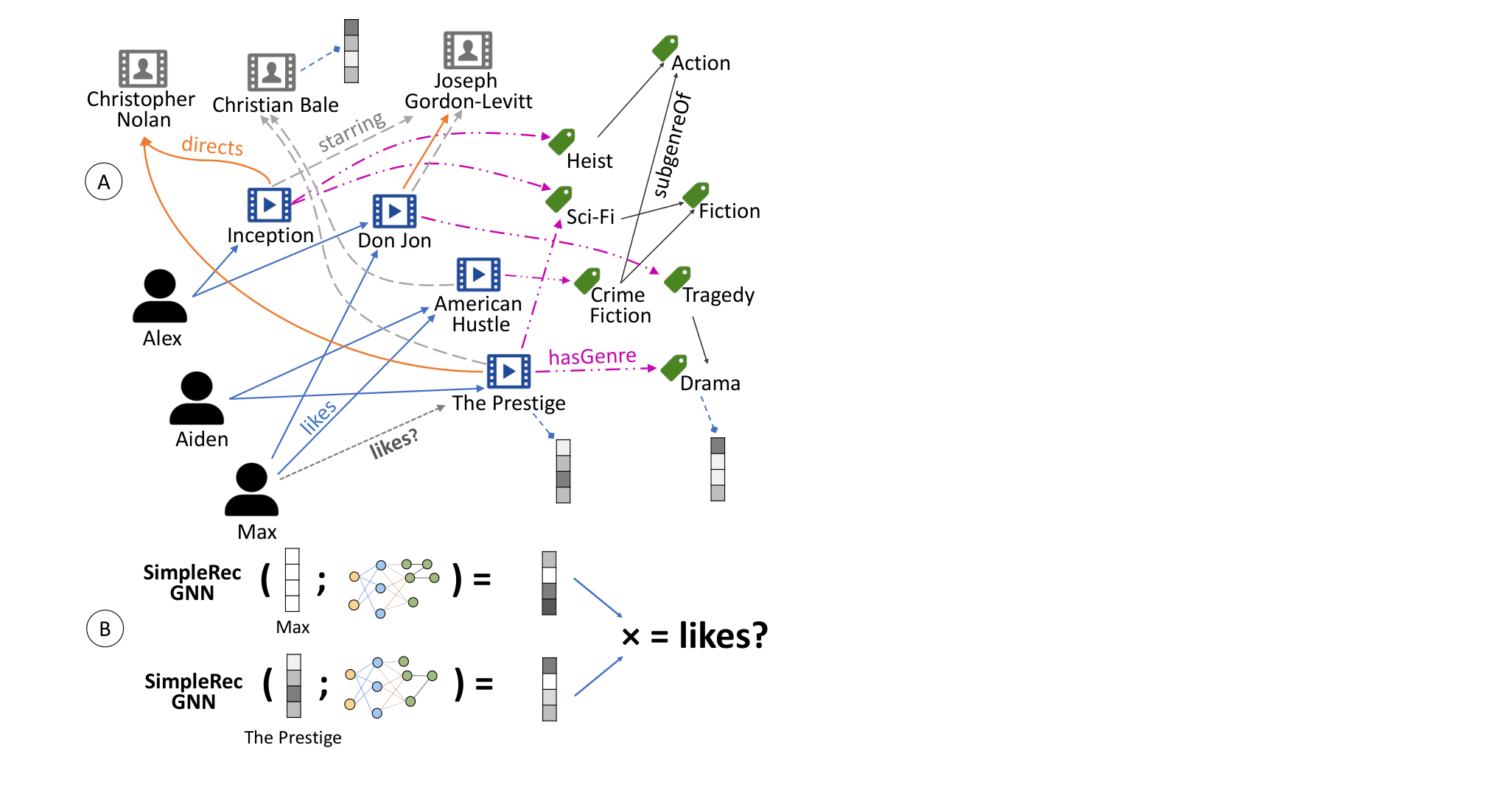
However, current inductive methods (Ying et al. 2018; Zhang and Chen 2019; Wu et al. 2021; Wang et al. 2021; Zhang et al. 2022; Zhang et al. 2021) only use interaction data, such as ratings, making them unable to handle situations where this type of data is sparse, e.g., long-tail users and items. Instead, including Knowledge Graph (KG)information would allow to handle long-tail users and items. Hence, we propose SimpleRec, a new simple-yet-powerful architecture that uses KGfor inductive predictions in a scalable way. Our baseline respects the following 4 important tenets: (i) it does not require any user metadata at all (e.g., personal attributes), (ii) it reduces the effect of the popularity bias by including both user-item information and item-entities connections11 1 The results in Appendix B illustrates this., (iii) it ensures scalability by avoiding the creation of any subgraph for each user-item pair and avoiding other complex sampling methods, and (iv) it exploits both relational information1 as well as any additional contextual information, e.g., textual attributes. As a result SimpleRecsets itself apart from trivial extensions of the GraphSAGE architecture as well as any other existing inductive method (Ying et al. 2018; Wang et al. 2019a; Wang et al. 2018a; Yang and Dong 2020; Palumbo et al. 2020; Wang et al. 2019c; Zhang and Chen 2019; Wu et al. 2021; Wang et al. 2021; Zhang et al. 2022; Zhang et al. 2021). We adopt this new strong baseline to re-evaluate state-of-the-art inductive recommendation methods. In doing so, we also put under scrutiny existing experimental protocols performed in previous studies. As a result, we identify also inconsistencies in previous evaluation protocols. Thus, our experiments show both a better way to evaluate Inductive Recommendation methods using KGs as well as an important scientific direction that has been evidently overlooked.
In the following, after providing the definition of recommendation over collaborative KGs, we illustrate issues with state-of-the-art methods for inductive recommendations, then we describe our proposed architecture, which we publish open-source along with the evaluation suite and re-implemented state-of-the-art methods at https://anonymous.4open.science/r/SimpleRec-DB4F. Finally, we present our evaluation methodology, overcoming existing issues, as well as the promising performances of our new proposed baseline.
2. Collaborative Knowledge Graphs
A KGis a heterogeneous graph representing entities as vertices (also nodes) and the semantic relations connecting them as labeled edges , given the relation types . In Figure 1, nodes represent recommendable items (), i.e., movies, and their connected entities (), e.g., actors, directors, and a taxonomy of genres, s.t. . Edges represent how nodes are connected, e.g., the entity “Inception” is connected to the genre “Heist” through the relation “has genre”. Furthermore, we adopt the concept of a Collaborative Knowledge Graph (CKG) (Wang et al. 2019a), i.e., a knowledge graph augmented with users () and user interactions, e.g., (Max, likes, Don Jon). We note that linking nodes in a KG also gives access to additional information that can be attached to nodes, e.g., encyclopedic texts about entities or product descriptions for items. Conversely, we explicitly avoid to assume any additional personal information about users, e.g., age or gender, as this information is usually not available and its storage constitutes more often a liability because of privacy concerns (Wang et al. 2018b).
In practice, we model our task as a top-k recommendation problem. We aim at learning a model that ranks items according to a user’s preferences estimated as ; i.e., , if user prefers item over . Furthermore, in line with previous literature (Wu et al. 2021; Zhang and Chen 2019; Lee et al. 2019), we define two types of users: warm-start users where some interactions are known at training time and cold-start users , for which no interaction is known at training time, but some become known at inference time. Thus, we only assume that entities in the KG itself remain unchanged, and we evaluate methods able to provide recommendation for the cold-start users.
3. Related Work
| Inductive | User | ||||||
| Model | User | Item | Metadata | Relational | Task | Subgraph | |
| NGCF (Wang et al. 2019b) | ✗ | ✗ | ✗ | ✗ | R | ✗ | |
| KGAT (Wang et al. 2019a) | ✗ | ✗ | ✗ | ✔ | R | ✗ | |
| KPRN (Wang et al. 2019c) | ✗ | ✗ | ✗ | ✔ | R | ✗ | |
| MeLU (Lee et al. 2019) | ✗ | ✗ | ✔ | ✗ | R | ✗ | |
| LGCN (He et al. 2020) | ✗ | ✗ | ✗ | ✗ | R | ✗ | |
| GraphSAGE (Hamilton et al. 2017) | (✔) | ✔ | ✗ | ✗ | C | ✗ | |
| PinSAGE (Ying et al. 2018) | (✔) | ✔ | ✗ | ✗ | R | ✗ | |
| IGMC (Zhang and Chen 2019) | ✔ | ✔ | ✗ | ✗ | P | ✔ | |
| IDCF (Wu et al. 2021) | ✔ | ✗ | ✗ | ✗ | P | ✗ | |
| PGD (Wang et al. 2021) | ✔ | ✔ | ✔ | ✗ | R | ✗ | |
| ICP (Zhang et al. 2021) | ✗ | ✔ | ✗ | ✗ | R | ✗ | |
| GIMC (Zhang et al. 2022) | ✔ | ✔ | ✗ | ✗ | P | ✔ | |
| SimpleRec | ✔ | ✔ | ✗ | ✔ | R | ✗ | |
Most existing recommendation methods are not able to represent nodes that were not present during training and are also limited in handling sparse datasets. First, most models are transductive, i.e., they embed each node in the graph within the same low-dimensionality space (Wang et al. 2019a; Wang et al. 2019c). Second, most of them utilize only bipartite graphs of user interactions with items (He et al. 2020; Wang et al. 2019b; Ying et al. 2018). Instead, inductive learning models generate predictions for unseen nodes by directly reasoning over the features that describe them. Here, we provide an overview of inductive methods, detailing their limitations as compared to our proposal (as summarized in Table 1).
GraphSAGE (Hamilton et al. 2017) was the first inductive Graph Neural Network (GNN)able to efficiently generate embeddings for unseen nodes by leveraging node features, e.g., textual attributes. It was later modified for the recommendation task in PinSAGE (Ying et al. 2018), also using MapReduce to scale the computation. Unfortunately, PinSAGE was designed for item-item recommendations, i.e., assuming we have boards of items and want to add a new item to a board. The method therefore does not explicitly handle user-item ratings but assumes that items closer in an embedding space will be rated similarly.
Other methods have been proposed for inductive matrix completion (Xu et al. 2013; Jain and Dhillon 2013), most recently IGMC (Zhang and Chen 2019) and GIMC (Zhang et al. 2022), which extract subgraphs around each user-item pair to obtain the necessary representations, passing such sub-graphs through multiple layers of a GNN. These approaches are designed for the single rating-prediction task and not for the ranking task. Generating these sub-graphs is prohibitively space- and time-consuming. Thus, they cannot efficiently produce user-item rankings, since a sub-graph is generated for all user-item pairs22 2 Similar to previous work (Wu et al. 2021) despite our best efforts, we were unable to train and test GIMC and IGMC in the ranking settings due to their running time requirements.. Furthermore, these methods do not use KG information; thus, they cannot provide predictions for new items with no interactions. Therefore, instead of constructing subgraphs, we employ subsampling of neighboring nodes to obtain a scalable prediction mechanism (Ying et al. 2018; Hamilton et al. 2017) and we use KGsto gain information also about items with few user interactions.
Some methods, e.g., PDG (Wang et al. 2021) and MeLU (Lee et al. 2019), exploit instead user metadata, e.g., gender and age information. Yet, this information is rarely available, making it impossible to use these methods in almost all cases33 3 We excluded MeLU as our tests without user metadata led to very poor results.. Moreover, MeLU (Lee et al. 2019) retrains the model for each user, which is not scalable. Hence, in our method, we assume no user metadata, learning instead how to aggregate information.
Related works therefore either: (i) create subgraphs, which do not scale in the ranking task; (ii) use personal user data, which is almost never available; or (iii) predict a single user rating, which under-performs in the ranking task, even compared to non-personalized methods (Cremonesi et al. 2010). Hence, (Table 1) only GraphSAGE (Hamilton et al. 2017), PinSAGE (Ying et al. 2018) and IDCF (Wu et al. 2021) are feasible methods to recommend for users that have not been seen during training, but they do not exploit KGs. Thus, we are the first to propose a scalable inductive method for user-personalized recommendation that learns to extract knowledge from a KG while not requiring any user metadata.
4. Inductive Relational GNN for Recommendation
We now present our architecture Simple and strong inductive baseline for Recommendation (SimpleRec), which is able to generate node vector representations for recommendation in an inductive manner for both users and items using a CKGwithout any user metadata. The model consists of three components: (i) an embedding layer, where we compress node feature information to create node embeddings (see Figure 2 A); (ii) a gated propagation layer, which chooses which information to propagate from the embeddings of neighboring nodes in a CKG(see Figure 2 C); and (iii) a prediction layer, which uses the output of all propagation layers to create a user and an item embedding, producing a ranking score (see Figure 2 D).
Embedding. As for other methods exploiting KGs (Hamilton et al. 2017; Ying et al. 2018), we assume most items and connected entities have textual information and employ node embedding techniques and node degrees as initial features. We use a pre-trained version of Sentence-BERT (Reimers and Gurevych 2019) to process the textual description of each entity and produce sentence embeddings. Nonetheless, when the non-recommendable entities are missing textual information, we can still learn their embeddings using Knowledge Graph Embedding (KGE)methods, since these entities are static (i.e., the KG excluding user and items, is not bound to change often). Specifically, we use ComplEX (Trouillon et al. 2016), trained with all triples in the KG, where we limit the output embeddings to be only on connected entities , while items are always represented using textual descriptions. Thus, we do not need retraining if new users or items are added. Yet, the initial features are too large () for the subsequent layers leading to out of memory errors and very slow training times. The dimensionality therefore has to be reduced before being passed to the GNNlayers. Hence, we introduce an AutoEncoder (AE)layer to reduce dimensionality (Kramer 1991). The loss of the AEis defined as:
| (1) |
where :, with , is the encoding function mapping the initial feature vector for each node to a set of lower dimensionality vectors. We define an AEfor each embedding type, i.e., one for textual embeddings and one for KGE, converting the embeddings into a shared embedding space. The output of the encoder is used as the input for the GNNs(see Figure 2 B).
Propagation. We apply multiple layers of GNNs (Hamilton et al. 2017; Ying et al. 2018). Yet, existing inductive GNN are not designed to use relational information. We therefore define relational gates as:
| (2) |
where defines the ego-network of node , is the gating function, and is the embedding of node . During the first graph convolution , i.e., the output dimensionality of the AE. In contrast to other gated networks (e.g., MGAT (Tao et al. 2020) and GGCN (Li et al. 2016)), our model’s gates are relation-specific, allowing it to propagate different information from different parts of an entity’s embedding based on the relation to it44 4 See Appendix B for the gating mechanism related improvements.. Hence, our gate is , with the sigmoid activation function , the concatenation operator , and .
The final part combines an entity’s current embedding with the aggregated ego-network embedding , defined as , where is an aggregator function. Among recent aggregators (Kipf and Welling 2016; Wang et al. 2019a; Hamilton et al. 2017), we identified the best performance with (He et al. 2020). We refer to Appendix A for the formal definition of the aggregators.
Prediction. As in previous approaches (Kipf and Welling 2016; Wang et al. 2019a; Tao et al. 2020), we concatenate the output after each layer for a user and item as: and efficiently obtaining the final prediction via dot-product as , which usually outperforms learned, non-linear, similarities (Rendle et al. 2020).
Optimization. The final loss function is a combination of autoencoder loss in Equation 1 and the Bayesian Personalized Ranking (BPR)loss (Wang et al. 2019a; He et al. 2020; Tao et al. 2020; Rendle et al. 2009), s.t. we learn to encode an embedding suitable for ranking while maintaining the information of the original features, computed as: , where and are tuned during hyperparameter optimization and are the learnable parameters. We study the effects of the AEloss in Appendix B.
| ML-20m | ML-S | AB | AB-S | ||||
|---|---|---|---|---|---|---|---|
| # Users | 132,287 | 12,500 | 70,679 | 60,000 | |||
| # Items | 4725 | 4438 | 24,841 | 24,841 | |||
| # Ratings | 11,376,533 | 1,106,000 | 847,733 | 720,111 | |||
| Density | 0.018 | 0.019 | 0.00048 | 0.00048 |
| Entities | Edges | Labels | Density | |
|---|---|---|---|---|
| MindReader (Brams et al. 2020) | 13,767 | 201,438 | 8 | 1.06e-3 |
| Amazon Book (Wang et al. 2019a) | 88,572 | 2,555,995 | 39 | 3.26e-4 |
Scalability. Our embedding approach, calculating the aggregation (), and the prediction () are all bounded by the number of nodes in the graph, while the calculation of the ego-network () is bounded by the number of edges. As these steps are applied sequentially and , we know that the complexity of our method is bounded by the ego-network aggregation complexity, more specifically, the linear transformation of the gate calculation. When naïvely applying the gates over all edges, the complexity is , where is the largest dimension utilized during graph convolutions55 5 We note that is bounded by .. Yet, as is equivalent to we only need to compute the transformation for each unique and pair instead of each unique triple. Therefore, we can apply a MapReduce computation (Ying et al. 2018) to have at most calculations, leading to the complexity .
As our prediction is a dot product after graph convolutions, our method can predict in for a single user as the vector dot product complexity is , which we do number of times. This is less than PinSAGE, which requires the dot product between all items and the user’s rated items, s.t. for a worst-case where a user has rated half the entities and we want to rank the other half. Our prediction is less computationally complex, as the reduced dimension, even when taking the number of layers into account as , is far less than the number of items.
5. Experiments
Inductive approaches are designed to provide recommendations in a cold-start setting, where ratings for new users are only known at inference time. Yet, as we will show, these baselines do not perform in this setting due to poor selection of learning metrics, evaluation methodologies, or other complexities. In the following, we aim at answering the questions: RQ1) Are existing inductive approaches really competitive when compared to SimpleRec? RQ2) Why do other architectures under-perform? and, RQ3) What negative item sampling strategy is the most appropriate for the evaluation?
| MovieLens Subsampled + 1250 users | MovieLens Subsampled + 90% | Amazon Book Subsampled + 15% | |||||||||||||
| NDCG | Recall | Precision | I-NDCG | NDCG | Recall | Precision | I-NDCG | NDCG | Recall | Precision | I-NDCG | ||||
| TopPop | 0.11182 | 0.14351 | 0.05256 | 0.85136 | 0.10916 | 0.14426 | 0.05147 | 0.85350 | 0.01552 | 0.03496 | 0.00273 | 0.78715 | |||
| GraphSAGE | 0.07862 | 0.10637 | 0.04336 | 0.84262 | 0.07281 | 0.10356 | 0.04164 | 0.84345 | 0.00667 | 0.01695 | 0.00149 | 0.76845 | |||
| PinSAGE | 0.14129 | 0.18745 | 0.06396 | 0.88378 | 0.13592 | 0.18622 | 0.06280 | 0.88496 | 0.05398 | 0.11764 | 0.00927 | 0.89937 | |||
| IDCF | 0.11042 | 0.14155 | 0.05244 | 0.81959 | 0.10875 | 0.14394 | 0.05113 | 0.85388 | 0.01205 | 0.02828 | 0.00231 | 0.75548 | |||
| SimpleRec | 0.18085* | 0.24618* | 0.08460* | 0.92200* | 0.18411* | 0.24482* | 0.08365* | 0.92208* | 0.06472* | 0.14055* | 0.01144* | 0.91769* | |||
Datasets. To evaluate existing methods, we adopt two real world datasets: (i) MovieLens-20m (ML-20m) (Harper and Konstan 2015), a dataset with ratings on movies and (ii) Amazon-Book (2014) (AB) (Ni et al. 2019), a dataset with reviews on books. Neither dataset has an associated KG. We therefore use the MindReader KG (Brams et al. 2020) for the ML-20mdataset, and for the ABdataset the KG constructed to evaluate KGAT (Wang et al. 2019a). In both cases, we keep only items mapped to the KG. We highlight how some methods compare performances over different versions of the ABdataset, e.g., the 2018 used in IDCF (Wu et al. 2021) is different from the version used in other works (Wang et al. 2019a; He et al. 2020; Wang et al. 2019b; for Recommender Systems 2022). Since users and items have an average of and ratings, respectively, on the 2018 dataset, while the users have an average of ratings and items in the 2014 dataset used here, our evaluation considers a sparse dataset, which is a more challenging setup. Therefore, comparisons on just the original reported numbers are unreliable.
In our cold-start experiments, we sample 12,500 users from ML-20mand 60,000 users from ABfor training, named MovieLens Subsampled (ML-S)and Amazon-Book Subsampled (AB-S), respectively. We then created two cold-start scenarios on ML-S: one adding 10% new users (i.e., 1250); and an extreme setting, where we treat all users not in ML-Sas cold-start users, being of the users in the original ML-20mdataset. For AB-Swe create one scenario adding the remaining users from the original dataset, being of total number of users.
Parameter settings. All models are implemented in PyTorch and optimized using the Adam optimizer66 6 We tested the methods’ implementations also on the datasets reported in their evaluation, when possible, getting similar results.; we train with a batch size of 1024 for a maximal of 1000 epochs, saving the best-performing state on the validation set and stopping after 50 successive epochs without improvement. For hyperparameter tuning, we employ Asynchronous Successive Halving (ASHA) (Li et al. 2018), with , , , setting minimum and maximum values of parameters based on the values described original works77 7 A configuration file can be found in the source code with all parameter options..
Methods. We compare to four methods: TopPop (Cremonesi et al. 2010), a simple non-personalized recommender that recommends the most popular items (a common baseline (Palumbo et al. 2020)); GraphSAGE (Hamilton et al. 2017), modified to recommend using the cosine similarity between a user’s rated items and new items; PinSAGE(Ying et al. 2018), with a semi-supervised objective, i.e., items co-rated should be similar, closely matching their pin/boards setting88 8 Based on https://github.com/dmlc/dgl/tree/master/examples/pytorch/pinsage; and IDCF (Wu et al. 2021), a two-step learning method, which reports experimental results superior to all other inductive methods to date.
RQ1 & RQ2. As Table 4 shows, SimpleRecis able to outperform all methods on all metrics with statistical significance. We also see contrasting results w.r.t. the original IDCF evaluation. IDCF was originally evaluated in a ranking setting; however, the learned embeddings of IDCF are learned towards Cross-Entropy, a non-ranking, point-wise learning objective. Such learning methodologies have been shown to perform poorly, learning a similar or worse ranking than TopPop (Cremonesi et al. 2010; Wu et al. 2022). In the original work, IDCF outperforms PinSAGE by a small margin, yet we observe the opposite in our evaluation. This is due to (i) our setup performing a more appropriate early stopping based on the evaluation metric instead of the loss function and (ii) our evaluation adopting a better learning objective for PinSAGE. Ranking loss generally leads to better performance, utilized by the two best performing methods. Yet, in IDCF method use the Cross-Entropy loss (Krichene and Rendle 2020).
RQ3. When evaluating ranking performance, NDCG is the metric commonly adopted, but there are two alternatives on which set of items to rank: either rank all items in the the dataset or just a subset. In other evaluations (Wu et al. 2021; He et al. 2017; Cremonesi et al. 2010), instead of ranking all items, only negative items are sampled per each positive. While this makes it equally hard to rank positive items for all test users, it has been proven to produce unreliable comparisons of performances across methods (Krichene and Rendle 2020). In the original IDCF evaluation, this faulty method (here labeled I-NDCG) is adopted. NDCG measures the methods’ ability to provide high-quality recommendations in the top of a ranked list. Yet, when subsampling negative items, the methods’ relative performance can change, meaning that the best performing method might not provide any or few relevant recommendations when challenged with the complete list of possible items. E.g., we see GraphSAGE outperforms IDCF on I-NDCG in both ML-S and AB-S, though clearly performing worse in the appropriate NDCG@20. On a different Amazon dataset, the Amazon-Beauty dataset, not reported here for space constraints, when utilizing the faulty I-NDCG, we also found TopPop (not included in the IDCF evaluation) outperforming all methods results (including IDCF) reported in IDCF (Wu et al. 2021). However, when using NDCG@20 we see up towards 3x times better performance when utilizing our method, compared to TopPop.
6. Conclusion and future work
In this work, we propose a simple and strong baseline for inductive recommendation. Our goal was to demonstrate the feasibility and advantages of this kind of architecture when compared to other inductive architectures. In particular, we devise a scalable GNN architecture to perform inductive learning for recommendation, able to utilize high-order connectivities in CKGs. We show that our method can outperform related work and showcase methodological limitations in the evaluation methods used. Overall, we conclude that more attention is needed towards this kind of architecture, especially given their ability to: (1) scale to large graphs and large numbers of users using MapReduce, and (2) maintain good prediction while being simple; i.e, performing no complex sampling methods or non-standard learning steps. Finally, we raise attention to the need for more sound evaluation protocols and for more transparency on the dataset adopted.
Acknowledgements
This research was partially funded by the Danish Council for Independent Research (DFF) under grant agreement no. DFF-8048-00051B and the Poul Due Jensen Foundation. During this work, Matteo Lissandrini was supported by the European Union’s Horizon 2020 research and innovation programme under the Marie Skłodowska-Curie grant agreement No 838216.
References
- (1)
- Brams et al. (2020) Anders H. Brams, Anders L. Jakobsen, Theis E. Jendal, Matteo Lissandrini, Peter Dolog, and Katja Hose. 2020. MindReader: Recommendation over Knowledge Graph Entities with Explicit User Ratings. In Proceedings of the 29th ACM International Conference on Information & Knowledge Management (Virtual Event, Ireland) (CIKM ’20). Association for Computing Machinery, New York, NY, USA, 2975–2982. https://doi.org/10.1145/3340531.3412759
- Cremonesi et al. (2010) Paolo Cremonesi, Yehuda Koren, and Roberto Turrin. 2010. Performance of recommender algorithms on top-n recommendation tasks. In Proceedings of the fourth ACM conference on Recommender systems. 39–46.
- for Recommender Systems (2022) BenchmArking for Recommender Systems. 2022. Bars Datasets. https://github.com/openbenchmark/BARS/tree/master/candidate_matching/datasets
- Hamilton et al. (2017) William L Hamilton, Rex Ying, and Jure Leskovec. 2017. Inductive representation learning on large graphs. In Proceedings of the 31st International Conference on Neural Information Processing Systems. 1025–1035.
- Harper and Konstan (2015) F Maxwell Harper and Joseph A Konstan. 2015. The movielens datasets: History and context. Acm transactions on interactive intelligent systems (tiis) 5, 4 (2015), 1–19.
- He et al. (2020) Xiangnan He, Kuan Deng, Xiang Wang, Yan Li, Yongdong Zhang, and Meng Wang. 2020. Lightgcn: Simplifying and powering graph convolution network for recommendation. In Proceedings of the 43rd International ACM SIGIR Conference on Research and Development in Information Retrieval. 639–648.
- He et al. (2017) Xiangnan He, Lizi Liao, Hanwang Zhang, Liqiang Nie, Xia Hu, and Tat-Seng Chua. 2017. Neural collaborative filtering. In Proceedings of the 26th international conference on world wide web. 173–182.
- Jain and Dhillon (2013) Prateek Jain and Inderjit S Dhillon. 2013. Provable inductive matrix completion. arXiv preprint arXiv:1306.0626 (2013).
- Kipf and Welling (2016) Thomas N Kipf and Max Welling. 2016. Semi-supervised classification with graph convolutional networks. arXiv preprint arXiv:1609.02907 (2016).
- Kramer (1991) Mark A Kramer. 1991. Nonlinear principal component analysis using autoassociative neural networks. AIChE journal 37, 2 (1991), 233–243.
- Krichene and Rendle (2020) Walid Krichene and Steffen Rendle. 2020. On Sampled Metrics for Item Recommendation. In Proceedings of the 26th ACM SIGKDD International Conference on Knowledge Discovery and Data Mining (Virtual Event, CA, USA) (KDD ’20). Association for Computing Machinery, New York, NY, USA, 1748–1757. https://doi.org/10.1145/3394486.3403226
- Lee et al. (2019) Hoyeop Lee, Jinbae Im, Seongwon Jang, Hyunsouk Cho, and Sehee Chung. 2019. Melu: Meta-learned user preference estimator for cold-start recommendation. In Proceedings of the 25th ACM SIGKDD International Conference on Knowledge Discovery & Data Mining. 1073–1082.
- Li et al. (2018) Liam Li, Kevin Jamieson, Afshin Rostamizadeh, Ekaterina Gonina, Moritz Hardt, Ben Recht, and Ameet Talwalkar. 2018. Massively parallel hyperparameter tuning. (2018).
- Li et al. (2016) Yujia Li, Daniel Tarlow, Marc Brockschmidt, and Richard S. Zemel. 2016. Gated Graph Sequence Neural Networks. In 4th International Conference on Learning Representations, ICLR 2016, San Juan, Puerto Rico, May 2-4, 2016, Conference Track Proceedings, Yoshua Bengio and Yann LeCun (Eds.). http://arxiv.org/abs/1511.05493
- Ni et al. (2019) Jianmo Ni, Jiacheng Li, and Julian McAuley. 2019. Justifying Recommendations using Distantly-Labeled Reviews and Fine-Grained Aspects. In Proceedings of the 2019 Conference on Empirical Methods in Natural Language Processing and the 9th International Joint Conference on Natural Language Processing (EMNLP-IJCNLP). Association for Computational Linguistics, Hong Kong, China, 188–197. https://doi.org/10.18653/v1/D19-1018
- Palumbo et al. (2020) Enrico Palumbo, Diego Monti, Giuseppe Rizzo, Raphaël Troncy, and Elena Baralis. 2020. entity2rec: Property-specific knowledge graph embeddings for item recommendation. Expert Systems with Applications 151 (2020), 113235.
- Reimers and Gurevych (2019) Nils Reimers and Iryna Gurevych. 2019. Sentence-BERT: Sentence Embeddings using Siamese BERT-Networks. In Proceedings of the 2019 Conference on Empirical Methods in Natural Language Processing and the 9th International Joint Conference on Natural Language Processing (EMNLP-IJCNLP). 3982–3992.
- Rendle et al. (2009) Steffen Rendle, Christoph Freudenthaler, Zeno Gantner, and Lars Schmidt-Thieme. 2009. BPR: Bayesian personalized ranking from implicit feedback. In Proceedings of the Twenty-Fifth Conference on Uncertainty in Artificial Intelligence. 452–461.
- Rendle et al. (2020) Steffen Rendle, Walid Krichene, Li Zhang, and John Anderson. 2020. Neural collaborative filtering vs. matrix factorization revisited. In Fourteenth ACM Conference on Recommender Systems. 240–248.
- Tao et al. (2020) Zhulin Tao, Yinwei Wei, Xiang Wang, Xiangnan He, Xianglin Huang, and Tat-Seng Chua. 2020. MGAT: Multimodal Graph Attention Network for Recommendation. Information Processing & Management 57, 5 (2020), 102277.
- Trouillon et al. (2016) Théo Trouillon, Johannes Welbl, Sebastian Riedel, Éric Gaussier, and Guillaume Bouchard. 2016. Complex Embeddings for Simple Link Prediction. In Proceedings of the 33nd International Conference on Machine Learning, ICML 2016, New York City, NY, USA, June 19-24, 2016 (JMLR Workshop and Conference Proceedings, Vol. 48), Maria-Florina Balcan and Kilian Q. Weinberger (Eds.). JMLR.org, 2071–2080. http://proceedings.mlr.press/v48/trouillon16.html
- Wang et al. (2018b) Cong Wang, Yifeng Zheng, Jinghua Jiang, and Kui Ren. 2018b. Toward privacy-preserving personalized recommendation services. Engineering 4, 1 (2018), 21–28.
- Wang et al. (2018a) Hongwei Wang, Fuzheng Zhang, Jialin Wang, Miao Zhao, Wenjie Li, Xing Xie, and Minyi Guo. 2018a. Ripplenet: Propagating user preferences on the knowledge graph for recommender systems. In Proceedings of the 27th ACM International Conference on Information and Knowledge Management. 417–426.
- Wang et al. (2021) Shuai Wang, Kun Zhang, Le Wu, Haiping Ma, Richang Hong, and Meng Wang. 2021. Privileged Graph Distillation for Cold Start Recommendation. In SIGIR ’21: The 44th International ACM SIGIR Conference on Research and Development in Information Retrieval, Virtual Event, Canada, July 11-15, 2021, Fernando Diaz, Chirag Shah, Torsten Suel, Pablo Castells, Rosie Jones, and Tetsuya Sakai (Eds.). ACM, 1187–1196. https://doi.org/10.1145/3404835.3462929
- Wang et al. (2019a) Xiang Wang, Xiangnan He, Yixin Cao, Meng Liu, and Tat-Seng Chua. 2019a. Kgat: Knowledge graph attention network for recommendation. In Proceedings of the 25th ACM SIGKDD International Conference on Knowledge Discovery & Data Mining. 950–958.
- Wang et al. (2019b) Xiang Wang, Xiangnan He, Meng Wang, Fuli Feng, and Tat-Seng Chua. 2019b. Neural graph collaborative filtering. In Proceedings of the 42nd international ACM SIGIR conference on Research and development in Information Retrieval. 165–174.
- Wang et al. (2019c) Xiang Wang, Dingxian Wang, Canran Xu, Xiangnan He, Yixin Cao, and Tat-Seng Chua. 2019c. Explainable reasoning over knowledge graphs for recommendation. In Proceedings of the AAAI Conference on Artificial Intelligence, Vol. 33. 5329–5336.
- Wu et al. (2022) Jiancan Wu, Xiang Wang, Xingyu Gao, Jiawei Chen, Hongcheng Fu, Tianyu Qiu, and Xiangnan He. 2022. On the Effectiveness of Sampled Softmax Loss for Item Recommendation. arXiv preprint arXiv:2201.02327 (2022).
- Wu et al. (2021) Qitian Wu, Hengrui Zhang, Xiaofeng Gao, Junchi Yan, and Hongyuan Zha. 2021. Towards Open-World Recommendation: An Inductive Model-based Collaborative Filtering Approach. In Proceedings of the 38th International Conference on Machine Learning, ICML 2021, 18-24 July 2021, Virtual Event (Proceedings of Machine Learning Research, Vol. 139), Marina Meila and Tong Zhang (Eds.). PMLR, 11329–11339. http://proceedings.mlr.press/v139/wu21j.html
- Xu et al. (2013) Miao Xu, Rong Jin, and Zhi-Hua Zhou. 2013. Speedup matrix completion with side information: Application to multi-label learning. In Advances in neural information processing systems. 2301–2309.
- Yang and Dong (2020) Zuoxi Yang and Shoubin Dong. 2020. HAGERec: hierarchical attention graph convolutional network incorporating knowledge graph for explainable recommendation. Knowledge-Based Systems 204 (2020), 106194.
- Ying et al. (2018) Rex Ying, Ruining He, Kaifeng Chen, Pong Eksombatchai, William L Hamilton, and Jure Leskovec. 2018. Graph convolutional neural networks for web-scale recommender systems. In Proceedings of the 24th ACM SIGKDD International Conference on Knowledge Discovery & Data Mining. 974–983.
- Zhang et al. (2022) Chengkun Zhang, Hongxu Chen, Sixiao Zhang, Guandong Xu, and Junbin Gao. 2022. Geometric Inductive Matrix Completion: A Hyperbolic Approach with Unified Message Passing. In WSDM ’22: The Fifteenth ACM International Conference on Web Search and Data Mining, Virtual Event / Tempe, AZ, USA, February 21 - 25, 2022, K. Selcuk Candan, Huan Liu, Leman Akoglu, Xin Luna Dong, and Jiliang Tang (Eds.). ACM, 1337–1346. https://doi.org/10.1145/3488560.3498402
- Zhang et al. (2021) Chuxu Zhang, Huaxiu Yao, Lu Yu, Chao Huang, Dongjin Song, Haifeng Chen, Meng Jiang, and Nitesh V Chawla. 2021. Inductive Contextual Relation Learning for Personalization. ACM Transactions on Information Systems (TOIS) 39, 3 (2021), 1–22.
- Zhang and Chen (2019) Muhan Zhang and Yixin Chen. 2019. Inductive Matrix Completion Based on Graph Neural Networks. In International Conference on Learning Representations.
Appendix A Aggregators
In the following we formally define the different aggregators used in the literature that we initially explored in our architecture.
- •
GCN aggregator (Kipf and Welling 2016) summing the two vectors and applying a nonlinear transformation:
(3) - •
GraphSAGE aggregator (Hamilton et al. 2017) concatenating the two vectors before applying a nonlinear transformation:
(4) - •
LightGCN aggregator (He et al. 2020) removing all transformations and simply propagating the ego-network vector:
(5)
Appendix B Ablation studies
We study the effect of different components and parameters in the cold-start setting. In particular, we investigate the effect of a gating mechanism, the autoencoder and using only a bipartite graph. In both Table 5 and Table 6, bold is the best performing method and ‘*’ signifies statistical significant improvement over the next best performing model. Furthermore we define Cov as
| (6) |
where is the set of the top-k items recommended given to a user . The naïve TopPop would always have a score of , while a random model would recommend all items given enough users, leading to a coverage score of . Intuitively, the metric therefore defines the diversity in a methods recommendations without taking the quality of the recommendations into account. We note that it is impossible to calculate statistical significance for coverage as all users have unique items and therefore does not change between methods.
B.1. Gating mechanism and KG structure
Gates. The results of the method with different gating mechanisms can be seen in Table 6. In the table, ‘w/o relation’ is the gating mechanism without relation type, i.e., a single type shared for all edges, and ‘w/o gates’ is the method without the gating mechanism.
- •
Overall, the gating mechanism improves performance, as we can adaptively select information from neighboring nodes seeing it outperform the two other models in all metrics.
- •
Disregarding relation types leads to worse performance on all datasets and completely removing the gates leads to dramatically lower performance.
- •
The models performance without gates is worse than PinSAGE, though still better than IDCF. Only using the users interactions without a gating mechanism, is therefore still better than the reconstruction using in IDCF.
- •
Even without relation types, we see large and statistical significant increase in performance. Allowing the model to select information based on itself and its neighbors are therefore very relevant for the models performance.
Effect of the KG. We create a version of the method where it only uses the collaborative graph instead of the CKG, named Bipartite in Table 6.
- •
We observe that the bipartite model performs very well on the ML-20mdataset, and less so on the ABdataset. The ABdataset is less dense making edges added by the KGmore important when clustering users according to their preferences.
- •
Even with its almost equivalent performance w.r.t. NDCG, the bipartite model lacks diversity. Furthermore, on all datasets, the SimpleRecwill outperform the bipartite model on at least one metric with statistical significance. On the ABwe see a large difference in the coverage of the model compared to the bipartite model. This is also visible on the ML-20mdatasets, though less prevalent.
- •
Combining the Cov and NDCG metric, we see that using KGinformation leads to more diverse recommendations without degrading the recommendation performance. Having highest diversity while having the highest ranking scores, means SimpleRecis able to recommend diverse and relevant items, with higher degree than without KGinformation. The recommendations are therefore less popularity biased when using KGinformation as it recommends a larger set of items.
B.2. Autoencoder
We study the impact of the AEloss, finding it to have minimal effect or decreasing performance (see Table 5). When comparing the best performing model where with the model where , we often see no statistical significant increase or decrease.
- •
We initially hypothesized that the encoded features trained without the AEloss would overfit and that the model would have a difficult time extracting relevant information through multiple GNNlayers. The AEloss would therefore help with extracting information while allowing the recommendation loss to tailor the encoded embedding to the recommendation setting. Yet, the results does not indicate that the AEloss improves the performance for our model.
- •
On the ML-20mand ABdatasets, we see a statistic significant decrease in performance between and . A high AEloss therefore does not give better recommendation capabilities.
- •
Lower values of either decreases performance or maintains it without statistical significant increases. We therefore leave it as future work to find out if it is possible to utilize the AEloss in a meaningful way for similar methods.
| MovieLens Subsampled + 1250 users | MovieLens Subsampled + 90% | Amazon Book Subsampled + 15% | ||||||||||
|---|---|---|---|---|---|---|---|---|---|---|---|---|
| NDCG | Recall | Precision | Cov | NDCG | Recall | Precision | Cov | NDCG | Recall | Precision | Cov | |
| 0.00 | 0.18123 | 0.18123 | 0.08292 | 0.19831 | 0.18367* | 0.24374* | 0.08335 | 0.44127 | 0.06842 | 0.14469 | 0.01171 | 0.20390 |
| 0.01 | 0.18013 | 0.23694 | 0.08232 | 0.20402 | 0.18260 | 0.24241 | 0.08320 | 0.43915 | 0.06745 | 0.14217 | 0.01141 | 0.17612 |
| 0.10 | 0.17642 | 0.23271 | 0.08152 | 0.17989 | 0.17947 | 0.23806 | 0.08138 | 0.37545 | 0.06812 | 0.14230 | 0.01166 | 0.24278 |
| 0.50 | 0.17708 | 0.23583 | 0.08076 | 0.17016 | 0.17818 | 0.23729 | 0.08139 | 0.33672 | 0.06861 | 0.14270 | 0.01170 | 0.22322 |
| 1.00 | 0.16832 | 0.22822 | 0.07860 | 0.15302 | 0.17339 | 0.23201 | 0.07925 | 0.29397 | 0.06251 | 0.13347 | 0.01089 | 0.18574 |
| 2.00 | 0.17089 | 0.22536 | 0.07736 | 0.14857 | 0.17295 | 0.23021 | 0.07838 | 0.27429 | 0.05939 | 0.12721 | 0.01034 | 0.13888 |
| MovieLens Subsampled + 1250 users | MovieLens Subsampled + 90% | Amazon Book Subsampled + 15% | ||||||||||
| NDCG | Recall | Precision | Cov | NDCG | Recall | Precision | Cov | NDCG | Recall | Precision | Cov | |
| Bipartite | 0.18331 | 0.24071 | 0.08264 | 0.17778 | 0.18379 | 0.24341 | 0.08309 | 0.42455 | 0.06386 | 0.13484 | 0.01108 | 0.18751 |
| W/o relations | 0.17720 | 0.24193 | 0.08288 | 0.18243 | 0.17799 | 0.23688 | 0.08140 | 0.34519 | 0.06451 | 0.13395 | 0.01106 | 0.18465 |
| W/o gates | 0.12482 | 0.17000 | 0.05848 | 0.08148 | 0.09416 | 0.13479 | 0.04331 | 0.05122 | 0.03653 | 0.00634 | 0.00927 | 0.07673 |
| SimpleRec | 0.18085 | 0.24618 | 0.08460* | 0.18540 | 0.18411 | 0.24482* | 0.08365* | 0.42646 | 0.06472 | 0.14055* | 0.01144* | 0.21460 |