Impact of Channel Aging on Reconfigurable Intelligent Surface Aided Massive MIMO Systems with Statistical CSI

Emerging applications bring challenges that demand ever-higher data rates and increased connectivity/coverage together with ultra-reliable and low-latency wireless communication (URLLC) requirements. Especially, these applications have led to the development of disruptive technologies such as massive multiple-input multiple-output (mMIMO) systems and millimeter-wave (mmWave) communications [1]. Unfortunately, existing techniques incur additional power and hardware costs while they cannot guarantee an adequate quality of service (QoS) in dead zones due to obstacles. For example, mMIMO exhibits poor performance in low scattering conditions, and the large number of active elements might result in prohibitive energy usage. In particular, they focus on improvements regarding the transmission and reception, while the wireless propagation environment is left uncontrollable. Furthermore, the time-varying and random nature of the wireless channel constitute the ultimate impediment to achieving the URLLC and rate targets.

In this direction, sixth generation (6G) networks, aiming at covering the higher rate demands and more stringent constraints, have appeared with the reconfigurable intelligent surface (RIS) being among its proposed promising technologies. Actually, RIS has attracted significant attention since it overcomes the aforementioned issues [2, 3, 4, 5, 6, 7, 8, 9, 10, 11, 12, 13]. Specifically, a RIS is a software-defined surface that is usually attached to existing infrastructure to alleviate blockage effects. It consists of a large number of individually-controlled, low-cost, and nearly passive elements. A RIS achieves to adapt to changes in the propagation environment and modify the radio waves since each of its elements can induce an adjustable phase shift to each incident signal, which enables a dynamic control over the wireless propagation channel. For instance, in [3], a minimization of the transmit power at the base station (BS) with signal-to-interference-plus-noise ratio (SINR) constraints took place in a RIS-assisted multi-user (MU) multiple-input single-output (MISO) communication system by jointly optimizing the precoding and reflecting beamforming matrices (RBMs). In [4], the sum rate was maximized subject to a transmit power constraint, while in [5], the sum rate was optimized by accounting also for correlated Rayleigh fading and inevitable hardware impairments at both the transceiver and the RIS. Similarly, in [6], the maximization of the minimum UE rate was studied in the case of a large number of antennas, in [7], the impact of hardware impairments was evaluated, and in [11], the impact of imperfect CSI on the outage probability was investigated. Notably, given that RIS-assisted MIMO systems, having a reduced number of active radio frequency (RF) chains, can achieve similar performance to mMIMO without RIS [13], it is indicated that a more cost and energy-efficient implementation of mMIMO is possible.

To reap the benefits of RIS and mMIMO and arrive at realistic conclusions, the acquisition of accurate channel state information (CSI) is of paramount importance [14, 15, 8, 16, 17, 18]. ¹¹ 1 Note that many previous works assumed perfect CSI, which is a highly unrealistic assumption. However, channel estimation (CE) in RIS-aided systems is quite challenging because of two main reasons. First, although its passive elements render RIS energy-efficient, they make infeasible conventional CE through transmitting and receiving pilots, which require active elements. Second, RIS generally includes a large number of elements, which require a prohibitively high training overhead that severely reduces the achievable rate. For instance, in [14], an ON/OFF CE scheme was proposed, where the least-squares estimates of all RIS-assisted MISO channels with a single user were calculated one by one. Moreover, other works such as [15, 8] do not provide analytical expressions for the estimated channel that could be exploited for the derivation of the spectral efficiency (SE). In [16], all RIS elements were assumed active during training but a number of sub-phases equal at least to the number of RIS elements are required, which results in a lower rate because the overhead on the coherence time for CE is larger. Moreover, this method does not provide the covariance of the estimated channel vector from all RIS elements to a specific UE but estimates of the individual channels while leaving the correlation among them unknown. An effective method with low overhead compared to previous works is to estimate the cascaded BS-RIS-UE channel in a single phase based on minimum mean square error (MMSE) as in [5]. Notably, another method, which reduces the overhead has been presented by exploiting RIS partitioning into subgroups, e.g., see [18]. Also, therein, an insightful categorization of the various CE approaches concerning RIS-assisted systems has been provided.

In practice, CSI is not only imperfect but can also be outdated because of channel aging [19, 20, 21, 22, 23]. The cause of channel aging is the UE mobility, which renders the channel time-varying, i.e., contrary to the standard block fading model, the channel evolves with time and is different during each symbol. Thus, a mismatch appears between the current channel and the estimated channel used for detection or precoding. Interestingly, in [22], channel aging was also considered during the training phase for a more realistic study. Several works have studied the impact of channel aging in mMIMO systems as mentioned but little attention has been given to its effect in RIS-assisted systems despite its great significance [23].

In principle, the phase shifts optimization lies on two methodologies with respect to CSI, namely, instantaneous CSI (I-CSI) [3, 4] and statistical CSI (S-CSI) [24, 6, 5, 25, 26, 23, 27, 28, 29]. The first approach suggests the optimization of the phases at every coherence interval because the related expressions depend on small-scale fading, while the second approach concerns expressions that depend on large-scale statistics, which vary every several coherence intervals. Hence, the latter approach enables considerably the reduction of the signal overhead and the computational complexity, which can become excessively high in the case of a large number of RIS elements and BS antennas. Moreover, for the same reasons, the S-CSI approach is more energy-efficient. Notably, in high mobility scenarios, which are faster time-varying, the I-CSI method would be very challenging to be implemented since the tuning of the RIS parameters should be repeated very frequently. On the contrary, the application of the S-CSI appears to be more practical.

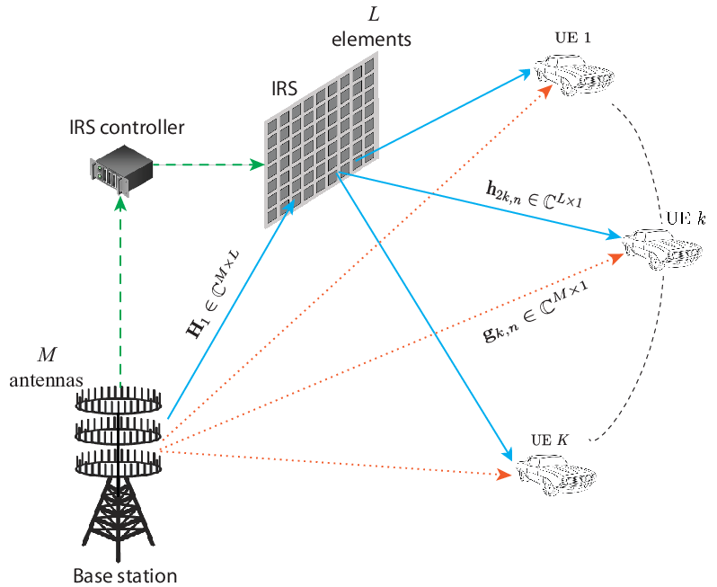
We consider a RIS-assisted downlink mMIMO system, where a BS, equipped with $M$ antennas communicates with $K$ single-antenna noncooperative UEs behind obstacles. A RIS, consisting of $L$ passive reflecting elements is located in the LoS of the BS to assist the communication with the UEs, e.g., imagine the common scenario where both the BS and RIS are deployed at high altitude and their locations are fixed, as shown in Fig. 1. The RIS can dynamically adjust the phase shift induced by each reflecting element on the impinging electromagnetic waves through a perfect smart controller that is connected to the BS in terms of a perfect backhaul link. The size of each RIS element is $d_{\mathrm{H}}\times d_{\mathrm{V}}$, where $d_{\mathrm{V}}$ and $d_{\mathrm{H}}$ express its vertical height and its horizontal width, respectively. The proposed model considers also the potential presence of direct links between the BS and the UEs. However, these could be also neglected in the cases of high penetration losses and/or big signal blockages.

Perfect CSI is not available in practice but the BS needs to estimate the channel. On this ground, we consider the standard time-division-duplex (TDD) protocol, where each block consists of $\tau$ channel uses for the uplink training phase and $\tau_{\mathrm{d}}=\tau_{\mathrm{c}}-\tau$ channel uses for the downlink data transmission phase [33]. The disadvantage of RIS-assisted systems is that the RIS, which consists of passive elements, cannot process the received pilot symbols from the UEs to obtain the estimated channels and cannot send pilots to the BS for CE. Herein, contrary to ON/OFF channel estimation schemes such as [14] and [16] that require $L+1$ phases, we perform the CE in a single phase. Notably, the consideration of the cascaded channel CE instead of the individual channels has already been applied in several works such as [5, 6]. Actually, it is more beneficial to consider the overall channel because this allows computing the correlation among inter-element links, while in the case of individual channels, this correlation remains unknown. Also, our CE is accompanied by reduced feedback and allows higher achievable SE due to the larger pre-log factor since the training overhead is much lower.

During the uplink training phase, each UE transmits a $\tau$-length mutually orthogonal training sequences, i.e., $\bm{\psi}_{k}=\left[\psi_{k,1},\ldots,\psi_{k,\tau}\right]^{{\scriptscriptstyle\mathsf{T}}}\in{\mathbb{C}}^{\tau\times 1}$. We assume that the pilot sequence consists of $K$ pilot symbols, which is the minimal number for channel estimation, i.e., $\tau\geq K$ [34]. Also, ${\bm{\Theta}}$ is assumed fixed. Thus, the received signal by the BS at time $n$ is given by

where $p_{\mathrm{p}}\geq 0$ is the common pilot transmit power for all UEs and ${\mathbf{W}}_{n}\in\mathbb{C}^{M\times\tau}$ is spatially white additive Gaussian noise matrix at the BS during this phase. After correlation of the received signal with the training sequence of UE $k$ $\frac{1}{\sqrt{p_{{\mathrm{p}}}}}{\bm{\psi}}_{k}$, we obtain

where $\tilde{{\mathbf{w}}}_{k,n}={\mathbf{W}}_{n}{\bm{\psi}}_{k}\sim\mathcal{CN}\left({\mathbf{0}},\tilde{\sigma}^{2}{\bm{\mathrm{I}}}_{M}\right)$.

Although this received signal can be used to estimate the channel at any time slot of the block, the estimated channel will deteriorate as the time interval between training and transmission increases. On this ground, we consider the channel estimate at $n=K+1$ since the estimate will be worse at a later instant. Based on (3), the channel at the $n$th instant ($n\leq K$) can be described in terms of the channel at time $K+1$ as

where $\tilde{{\mathbf{e}}}_{k,n}\sim\mathcal{CN}\left({\mathbf{0}},{\mathbf{R}}_{k}\right)$ is the independent innovation vector, which relates ${\mathbf{h}}_{k,n}$ and ${\mathbf{h}}_{k,\zeta}$. Also, we have defined $\zeta=K+1$ to simplify the notation. Inserting (6) into (5), we obtain

By applying the standard minimum mean square error (MMSE) estimation [33], the BS obtains the channel estimate of ${{\mathbf{h}}}_{k,\zeta}$ as

where ${\mathbf{Q}}=\left({\mathbf{R}}_{k}+\frac{\tilde{\sigma}^{2}}{{p_{{\mathrm{p}}}}}{\bm{\mathrm{I}}}_{M}\right)^{-1}$. The estimate $\hat{{\mathbf{h}}}_{k,\zeta}$ is distributed as $\mathcal{CN}\left({\mathbf{0}},{\bm{\Phi}}_{k}\right)$, where ${\bm{\Phi}}_{k}=\alpha^{2}_{k,\zeta-n}{\mathbf{R}}_{k}{\mathbf{Q}}{\mathbf{R}}_{k}$. According to the orthogonality property of MMSE estimation, the independent channel estimation error vector is $\tilde{{\mathbf{h}}}_{k,\zeta}={{\mathbf{h}}}_{k,\zeta}-\hat{{\mathbf{h}}}_{k,\zeta}$ and distributed as $\mathcal{CN}\left({\mathbf{0}},{\bm{\Psi}}_{k}\right)$, where ${\bm{\Psi}}_{k}={\mathbf{R}}_{k}-{\bm{\Phi}}_{k}$. Notably, the channel estimate $\hat{{\mathbf{h}}}_{k,\zeta}$ in (8) includes the degradation due to the channel aging.

In Sec. VI, we illustrate the normalized mean square error (NMSE) defined as

According to (10), an increase in channel aging results in the increase of the $\mathrm{NMSE}_{k}$. Overall, channel aging has a detrimental on channel estimation. Below, we elaborate on its impact during the downlink transmission.

The downlink transmission of data from the BS to all UEs consists of a broadcast channel that has to make use of a certain precoding strategy in terms of a precoding vector ${\mathbf{f}}_{k,n}\in{\mathbb{C}}^{M\times 1}$. In parallel, taking advantage of TDD and its channel reciprocity, the downlink channel is the Hermitian transpose of the uplink channel. Thus, the received signal $r_{k,n}\in{\mathbb{C}}$ by UE $k$ during the data transmission phase ($n=K+1,\ldots,\tau_{\mathrm{c}}$) can be written as

where ${\mathbf{s}}_{n}=\sum_{i=1}^{K}\sqrt{p_{i}}{\mathbf{f}}_{i,n}x_{i,n}$ describes the transmit signal vector by the BS, $p_{i}\geq 0$ is the transmit power to UE $i$, and $z_{k,n}\sim{\cal C}{\cal N}(0,\sigma^{2})$ is complex Gaussian noise at UE $k$. Note that ${\mathbf{f}}_{i,n}\in{\mathbb{C}}^{M\times K}$ and $x_{i,n}$ are the linear precoding vector and the data symbol with $\mathbb{E}\{|x_{i,n}|^{2}\}=1$, respectively.⁶⁶ 6 If we assume that mmWwave communication takes place, hybrid beamforming can be introduced as the best solution that achieves a good trade-off between cost and complexity as usually adopted in the literature. However, the study of the impact of channel aging in the mmWwave region is left for future research due to limited space. The precoding vector is normalized based on the average total power constraint

where ${\mathbf{F}}_{n}=[{\mathbf{f}}_{1,n},\ldots,{\mathbf{f}}_{K,n}]\in\mathbb{C}^{M\times K}$, ${\mathbf{P}}=\text{diag}(p_{1},\ldots,p_{K})$, and $P_{\mathrm{max}}>0$ is the total transmit power. However, the channel ${\mathbf{h}}_{k,n}$ in (11) can be expressed as

where $\hat{{\mathbf{h}}}_{k}$ expresses the channel vector at the beginning of the data transmission phase, and $\tilde{{\mathbf{h}}}_{k}$ is the corresponding channel estimation error.

Substitution of (13) into (11) provides

Although UEs do not have instantaneous CSI, we can assume that UE $k$ has access to $\mathbb{E}\{\hat{{\mathbf{h}}}_{k}^{{\scriptscriptstyle\mathsf{H}}}{\mathbf{f}}_{k,n}x_{k,n}\}$. Then, by using the technique in [35], where UE $k$ is aware of only the statistical CSI, the received signal is written as

In this section, we focus on the optimization of the sum SE of a RIS-assisted time-varying mMIMO system with channel aging. Specifically, the sum rate maximization problem is described as

where we have denoted the elements of ${\bm{\Theta}}$ as $\tilde{\theta}_{l}=\exp\left(j\theta_{l}\right)$ for all $l$ and the vector ${\mathbf{p}}=[p_{1},\ldots,p_{K}]^{{\scriptscriptstyle\mathsf{T}}}$. The first constraint in (24b) means that each RIS element induces a phase shift without any change on the amplitude of the incoming signal, while constraint (24c) ensures that the BS transmit power is kept below the maximum power $P_{\mathrm{max}}$.⁹⁹ 9 The considered optimization problem allocates the available resources (power vector, RIS configuration) to maximize the total spectral efficiency (i.e, sum-rate). This is a well-known objective function when the total/aggregate rate of the network is the key design priority. It is worth also noting that the sum capacity/rate is a fundamental performance metric (one dimension) in multi-user networks from information theoretic perspective. To consider QoS per individual user, the consideration of other objective functions that take into account fairness (e.g. max-min rate) and/or minimum individual rates is required, which are beyond the scope of this paper and can be considered for future work.

The solution of the optimization problem $(\mathcal{P}1)$ is challenging due to its non-convexity and the unit-modulus constraint concerning $\tilde{\theta}_{l}$. To tackle this difficulty, we consider the alternating optimization (AO) technique, where ${\bm{\Theta}}$ and ${\mathbf{p}}$ are going to be solved separately and iteratively. In particular, first, we focus on finding the optimum ${\bm{\Theta}}$ given fixed ${\mathbf{p}}$. Next, we solve for ${\mathbf{p}}$ with fixed ${\bm{\Theta}}$. The iteration of this procedure, where the sum rate increases at each iteration step, continues until convergence to the optimum value since the sum rate is upper-bounded subject to the power constraint (24c). Note that all computations take place at the BS.

References

- [1] F. Boccardi et al., “Five disruptive technology directions for 5G,” IEEE Commun. Mag., vol. 52, no. 2, pp. 74–80, 2014.
- [2] E. Basar et al., “Wireless communications through reconfigurable intelligent surfaces,” IEEE Access, vol. 7, pp. 116 753–116 773, 2019.
- [3] Q. Wu and R. Zhang, “Intelligent reflecting surface enhanced wireless network via joint active and passive beamforming,” IEEE Trans. Wireless Commun., vol. 18, no. 11, pp. 5394–5409, 2019.
- [4] C. Pan et al., “Multicell MIMO communications relying on intelligent reflecting surfaces,” IEEE Trans. Wireless Commun., vol. 19, no. 8, pp. 5218–5233, 2020.
- [5] A. Papazafeiropoulos et al., “Intelligent reflecting surface-assisted MU-MISO systems with imperfect hardware: Channel estimation, beamforming design,” IEEE Trans. Wireless Commun., 2021.
- [6] A. Kammoun et al., “Asymptotic max-min SINR analysis of reconfigurable intelligent surface assisted MISO systems,” IEEE Trans. Wireless Commun., vol. 19, no. 12, pp. 7748–7764, 2020.
- [7] A. Papazafeiropoulos et al., “Asymptotic analysis of Max-Min weighted SINR for IRS-assisted MISO systems with hardware impairments,” IEEE Wireless Commun. Lett., pp. 1–1, 2021.
- [8] A. M. Elbir et al., “Deep channel learning for large intelligent surfaces aided mm-Wave massive MIMO systems,” IEEE Wireless Commun. Lett., vol. 9, no. 9, pp. 1447–1451, 2020.
- [9] H. Guo et al., “Weighted sum-rate maximization for reconfigurable intelligent surface aided wireless networks,” IEEE Trans. Wireless Commun., vol. 19, no. 5, pp. 3064–3076, 2020.
- [10] J. Chen et al., “Intelligent reflecting surface: A programmable wireless environment for physical layer security,” IEEE Access, vol. 7, pp. 82 599–82 612, 2019.
- [11] P. Yang, L. Yang, and S. Wang, “Performance analysis for RIS-Aided Wireless Systems With Imperfect CSI,” IEEE Wireless Commun. Lett., vol. 11, no. 3, pp. 588–592, 2021.
- [12] E. Björnson, Ö. Özdogan, and E. G. Larsson, “Intelligent reflecting surface versus decode-and-forward: How large surfaces are needed to beat relaying?” IEEE Wireless Commun. Lett., vol. 9, no. 2, pp. 244–248, 2019.
- [13] M. Di Renzo et al., “Smart radio environments empowered by reconfigurable intelligent surfaces: How it works, state of research, and the road ahead,” IEEE J. Sel. Areas Commun., vol. 38, no. 11, pp. 2450–2525, 2020.
- [14] D. Mishra and H. Johansson, “Channel estimation and low-complexity beamforming design for passive intelligent surface assisted MISO wireless energy transfer,” in International Conference on Acoustics, Speech and Signal Processing (ICASSP). IEEE, 2019, pp. 4659–4663.
- [15] Z.-Q. He and X. Yuan, “Cascaded channel estimation for large intelligent metasurface assisted massive MIMO,” IEEE Wireless Commun. Lett., vol. 9, no. 2, pp. 210–214, 2019.
- [16] Q. Nadeem et al., “Intelligent reflecting surface-assisted multi-user MISO Communication: Channel estimation and beamforming design,” IEEE Open J. Commun. Soc., vol. 1, pp. 661–680, 2020.
- [17] B. Zheng and R. Zhang, “Intelligent reflecting surface-enhanced OFDM: Channel estimation and reflection optimization,” IEEE Wireless Commun. Lett., vol. 9, no. 4, pp. 518–522, 2019.
- [18] E. Shtaiwi et al., “Channel estimation approach for RIS assisted MIMO systems,” IEEE Trans. Cogn. Commun. Net., vol. 7, no. 2, pp. 452–465, 2021.
- [19] K. Truong and R. Heath, “Effects of channel aging in massive MIMO systems,” IEEE/KICS J. Commun. Net., Special Issue on massive MIMO, vol. 15, no. 4, pp. 338–351, Aug 2013.
- [20] A. K. Papazafeiropoulos and T. Ratnarajah, “Deterministic equivalent performance analysis of time-varying massive MIMO systems,” IEEE Trans. Wireless Commun., vol. 14, no. 10, pp. 5795–5809, 2015.
- [21] A. K. Papazafeiropoulos, “Impact of general channel aging conditions on the downlink performance of massive MIMO,” IEEE Trans. Veh. Tech., vol. 66, no. 2, pp. 1428–1442, Feb 2017.
- [22] R. Chopra et al., “Performance analysis of FDD massive MIMO systems under channel aging,” IEEE Trans. Wireless Commun., vol. 17, no. 2, pp. 1094–1108, 2017.
- [23] Y. Chen, Y. Wang, and L. Jiao, “Robust transmission for reconfigurable intelligent surface aided millimeter wave vehicular communications with statistical CSI,” IEEE Trans. Wireless Commun., pp. 1–1, 2021.
- [24] M.-M. Zhao et al., “Intelligent reflecting surface enhanced wireless network: Two-timescale beamforming optimization,” IEEE Trans. Wireless Commun., vol. 19, no. 8, pp. 5218–5233, 2020.
- [25] T. Van Chien et al., “Outage probability analysis of IRS-assisted systems under spatially correlated channels,” IEEE Wireless Commun. Lett., pp. 1–1, 2021.
- [26] A. Papazafeiropoulos et al., “Coverage probability of distributed IRS systems under spatially correlated channels,” IEEE Wireless Commun Lett., pp. 1–1.
- [27] L. You et al., “Reconfigurable intelligent surfaces-assisted multiuser MIMO Uplink Transmission With Partial CSI,” IEEE Trans. Wireless Commun., vol. 20, no. 9, pp. 5613–5627, 2021.
- [28] K. Zhi et al., “Power scaling law analysis and phase shift optimization of RIS-Aided Massive MIMO Systems With Statistical CSI,” IEEE Trans. Commun., vol. 70, no. 5, pp. 3558–3574, 2022.
- [29] Y. Zhang et al., “Performance analysis of reconfigurable intelligent surface assisted systems under channel aging,” Intelligent and Converged Networks, vol. 3, no. 1, pp. 74–85, 2022.
- [30] E. Björnson and L. Sanguinetti, “Rayleigh fading modeling and channel hardening for reconfigurable intelligent surfaces,” IEEE Wireless Commun. Lett., vol. 10, no. 4, pp. 830–834, 2021.
- [31] D. Neumann, M. Joham, and W. Utschick, “Covariance matrix estimation in massive MIMO,” IEEE Signal Process. Lett., vol. 25, no. 6, pp. 863–867, 2018.
- [32] S. Abeywickrama et al., “Intelligent reflecting surface: Practical phase shift model and beamforming optimization,” IEEE Trans. Commun., vol. 68, no. 9, pp. 5849–5863.
- [33] E. Björnson, J. Hoydis, and L. Sanguinetti, “Massive MIMO networks: Spectral, energy, and hardware efficiency,” Foundations and Trends® in Signal Processing, vol. 11, no. 3-4, pp. 154–655, 2017.
- [34] B. Hassibi and B. Hochwald, “How much training is needed in multiple-antenna wireless links?” IEEE Trans. Inform. Theory, vol. 49, no. 4, pp. 951–963, April 2003.
- [35] M. Medard, “The effect upon channel capacity in wireless communications of perfect and imperfect knowledge of the channel,” IEEE Trans. Inf. Theory, vol. 46, no. 3, pp. 933–946, May 2000.
- [36] E. Björnson, M. Matthaiou, and M. Debbah, “Massive MIMO with non-ideal arbitrary arrays: Hardware scaling laws and circuit-aware design,” IEEE Trans. Wireless Commun., vol. 14, no. 8, pp. 4353–4368, Aug 2015.
- [37] A. Pitarokoilis, S. Mohammed, and E. Larsson, “Uplink performance of time-reversal MRC in massive MIMO systems subject to phase noise,” IEEE Trans. Wireless Commun., vol. 14, no. 2, pp. 711–723, Feb 2015.
- [38] J. Hoydis, S. ten Brink, and M. Debbah, “Massive MIMO in the UL/DL of cellular networks: How many antennas do we need?” IEEE J. Select. Areas Commun., vol. 31, no. 2, pp. 160–171, February 2013.
- [39] R. Couillet and M. Debbah, Random matrix methods for wireless communications. Cambridge University Press, 2011.
- [40] S. Boyd, S. P. Boyd, and L. Vandenberghe, Convex optimization. Cambridge university press, 2004.
- [41] Q. Shi et al., “An iteratively weighted MMSE approach to distributed sum-utility maximization for a MIMO interfering broadcast channel,” vol. 59, no. 9, pp. 4331–4340, 2011.
- [42] E. Access, “Further advancements for E-UTRA physical layer aspects,” 3GPP Technical Specification TR, vol. 36, p. V2, 2010.
- [43] Z. Bai and J. W. Silverstein, Spectral analysis of large dimensional random matrices. Springer, 2010, vol. 20.
- [44] S. Wagner et al., “Large system analysis of linear precoding in correlated MISO broadcast channels under limited feedback,” IEEE Trans. Inf. Theory, vol. 58, no. 7, pp. 4509–4537, July 2012.
- [45] R. Krishnan et al., “Linear massive MIMO precoders in the presence of phase noise-A large-scale analysis,” IEEE Trans. Veh. Tech., vol. 65, no. 5, pp. 3057–3071, 2016.
- [46] K. B. Petersen and M. S. Pedersen, “The matrix cookbook, nov 2012,” URL http://www2. imm. dtu. dk/pubdb/p. php, vol. 3274, p. 14, 2012.