In this section, we briefly introduce the concept of $L^{p}$ graphons pioneered by Borgs et al., 2018 and Borgs et al., 2019 which provide more details. $L^{p}$ graphons can be informally thought of as adjacency matrices for graphs with (almost) infinitely many nodes. Naturally, approximating sparse finite graphs by these $L^{p}$ graphons leads to the loss of some topological information, see e.g. Borgs et al., 2018. Nevertheless, $L^{p}$ graphons provide an expressive asymptotic approximation of the finite case which we show both theoretically and empirically on the next pages. In contrast to standard graphons which are limited to dense graphs, $L^{p}$ graphons are more general and also apply to sparse graphs. An $L^{p}$ graphon is a symmetric, integrable function $W\colon\left[{0,1}\right]^{2}\rightarrow\mathbb{R}$ with $\left\|{W}\right\|_{p}<\infty$ where the $L^{p}$ norm on graphons is $\left\|{W}\right\|_{p}\coloneqq\left({\int_{\left[{0,1}\right]^{2}}\left|{W(x,y)}\right|^{p}\,\mathrm{d}x\,\mathrm{d}y}\right)^{1/p}$ for $1\leq p<\infty$ and the essential supremum if $p=\infty$.

To quantify whether a graphon is a good approximation for a sequence of finite graphs, we associate every finite graph $G=\left({V(G),E(G)}\right)$ with a graphon $W^{G}$. For a graph $G$ with $N$ nodes, we partition the unit interval $[0,1]$ into $N$ intervals $I_{1},\ldots,I_{N}$ of equal length. Then, the function $W^{G}$ is assigned a constant value on each square $I_{i}\times I_{j}$ ($i,j\in V(G)$) which is equal to one if there is an edge between the nodes $i,j$ in $G$ and zero otherwise. Thus, $W^{G}$ is by construction a step-function and therefore often called step-graphon. To compare some graph $G$ and graphon $W$, we can simply compare the graphons $W$ and $W^{G}$ in the space of graphons. Instead of $W^{G}$ itself, we frequently consider the normalized associated graphon $W_{G}/\left\|{G}\right\|_{1}$ to derive results that also hold in the sparse case. To measure how close two graphons are, the cut norm is a natural candidate and possesses many useful properties, see e.g. Lovász, 2012 for a detailed discussion. For a graphon $W\colon\left[{0,1}\right]^{2}\rightarrow\mathbb{R}$, define the cut norm by

where $S$ and $T$ range over the measurable subsets of $\left[{0,1}\right]$.

Starting with a graphon, we can use the following well-established construction to generate sparse random graphs with $N$ nodes where we assume without loss of generality that the vertices are labeled by $1,\ldots,N$. We choose $x_{1},\ldots,x_{N}$ i.i.d. uniformly at random in $[0,1]$ and fix some $\rho>0$. For all vertex pairs $1\leq i<j\leq N$ there is an edge between $i$ and $j$ with probability $\min\left\{{\rho W(x_{i},x_{j}),1}\right\}$ which yields a sparse random graph $\mathbf{G}\left({N,W,\rho}\right)$. A sequence of sparse random graphs generated by this method converges to the generating graphon $W$ in the cut norm, see (Borgs et al., 2019, Theorem 2.14).

The limiting graphon in Assumption 1 is only guaranteed to exist for so-called $L^{p}$ upper regular graph sequences, for details see Borgs et al., 2018, Borgs et al., 2019. This implicit assumption means that our approach does not apply to arbitrary sequences of sparse random graphs. If the average degree in the graph sequence does not tend to infinity as $N\to\infty$, $L^{p}$ upper regularity is not fulfilled. Thus, for example, the asymptotic behavior of ultra-sparse graph sequences is beyond the scope of $L^{p}$ graphons. Nevertheless, $L^{p}$ graphons are the limit of crucial sparse graph sequences such as power law graphs which cannot be provided by standard graphons. In our paper, ’power law’ refers to the tail of the distribution. Figure 1 shows the advantages of $L^{p}$ graphons over standard graphons using an exemplary real-world network (data from Rozemberczki et al., 2019). The examples in the next sections are usually based on power law graphons $W\colon\left[{0,1}\right]^{2}\rightarrow\mathbb{R}$ with $W(x,y)=(1-\alpha)^{2}(xy)^{-\alpha}$ where $\alpha\in(0,1)$, see Borgs et al., 2018 for details.

For the theoretical analysis of the OMD algorithm in the next sections, we introduce the concept of smoothed step graphons which is new to the best of our knowledge. The basic idea is to smooth the borders of the steps. Then, the smoothed step graphon is Lipschitz continuous but still close to the original step graphon as we decrease the width $\xi$ of the border regions.

Consider an arbitrary step graphon $W_{s}$ on the unit interval partitioned into $M$ subintervals $\mathcal{I}_{1},\ldots,\mathcal{I}_{M}$ of equal length $1/M$ such that $W_{s}(x,y)=w_{i,j}\geq 0$ for all $(x,y)\in\mathcal{I}_{i}\times\mathcal{I}_{j},1\leq i,j\leq M$. Then, for an arbitrary but fixed $0<\xi<1/(2M)$, we define the corresponding smoothed step graphon $W_{s,\xi}$ as follows. For all $(x,y)\in\left\{(x,y)\in[0,1]^{2}:(x\leq\xi)\lor(x\geq 1-\xi)\right\}$ and $(x,y)\in\left\{(y\leq\xi)\lor(y\geq 1-\xi)\right\}$ we define $W_{s,\xi}(x,y)\coloneqq W_{s}(x,y)$. The values of the two graphons are also defined to be identical for $(x,y)$ with $(x,y)\in\widetilde{\mathcal{I}}_{i}\times\widetilde{\mathcal{I}}_{j}$ for some $1\leq i,j\leq M$ where $\widetilde{\mathcal{I}}_{i}\coloneqq[(i-1)/M+\xi,i/M-\xi)$ for all $1\leq i\leq M$. In contrast to that, if $x\in\widetilde{\mathcal{I}}_{i}$ and $y\in[j/M-\xi,j/M+\xi)$ for some $1\leq i,j\leq M$, we have $W_{s,\xi}(x,y)\coloneqq(\frac{1}{2}-\frac{y-j/M}{2\xi})w_{i,j}+\frac{y-j/M+\xi}{2\xi}w_{i,j+1}$ and analogously for $x$ and $y$ with switched roles. Finally, if both $x\in[i/M-\xi,i/M+\xi)$ and $y\in[j/M-\xi,j/M+\xi)$ for some $1\leq i,j\leq M$, we define

Note that $W_{s,\xi}$ is Lipschitz continuous and that by construction we have $\left\|{W_{s,\xi}-W_{s}}\right\|_{\square}\leq 4M\xi\cdot\max_{i,j}w_{i,j}$ which approaches zero as $\xi\to 0$.

For the finite case, we assume that there are $N$ agents with finite state and action spaces $\mathcal{X}$ and $\mathcal{U}$, respectively. The agents implement actions at time points $\mathcal{T}\coloneqq\left\{{0,\ldots,T-1}\right\}$ with terminal time point $T$. The interactions between individuals are modeled by a graph $G_{N}=(V_{N},E_{N})$ where each vertex represents one agent and each edge a connection between two agents. For an arbitrary finite set $A$ we denote by $\mathcal{P}(A)$ the set of all probability measures on $A$ and by $\mathcal{B}(A)$ the set of all bounded measures on $A$. Thus, the space of policies is defined as $\Pi\coloneqq\mathcal{P}(\mathcal{U})^{\mathcal{T}\times\mathcal{X}}$ and a policy of agent $i$ is denoted by $\pi^{i}=\left({\pi^{i}_{t}}\right)_{t\in\mathcal{T}}\in\Pi$ correspondingly. Furthermore, agents in the model are assumed to implement Markovian feedback policies such that they only consider local state information. Formally, this is captured by defining for all $t\in\mathcal{T}$ and $i\in V_{N}$ the model dynamics

with $X^{i}_{0}\sim\mu_{0}$ for some transition kernel $P\colon\mathcal{X}\times\mathcal{U}\times\mathcal{B}(\mathcal{X})\to\mathcal{P}(\mathcal{X})$ and the neighborhood state distribution

for each agent $i$ with $\delta$ being the Dirac measure and $\mathbb{G}^{i}_{t}\in\mathcal{B}(\mathcal{X})$ for all $i\leq N$ by definition. The normalization factor $\rho_{N}$ ensures that the neighborhood distribution does not converge to a vector of zeros as $N$ approaches infinity. Here, $\rho_{N}$ is assumed to have the same asymptotic order as the edge density of $G_{N}$, i.e. $\rho_{N}=\Theta\left({\left|{E_{N}}\right|/N^{2}}\right)$ as $N\to\infty$. Each agent faces a reward function $r\colon\mathcal{X}\times\mathcal{U}\times\mathcal{B}(\mathcal{X})\to\mathbb{R}$ which yields her reward depending on her state, action, and the state distribution of her neighbors. Agents competitively try to maximize their expected sum of rewards

Note that we can handle the infinite-horizon discounted objective case analogously, see e.g. Cui and Koeppl, 2022. Finding equilibria for this type of model requires a suitable equilibrium concept. Although the classical Nash equilibrium notion (see, e.g. Carmona and Delarue, 2018a) seems to be a natural candidate, its definition requires that no agent has an incentive to unilaterally deviate from the current policy. As we are primarily interested in an approximation via $L^{p}$ graphons, this equilibrium concept is to strict. Even in the limit $N\to\infty$ there can always occur (small) subgroups of agents whose graph connections deviate from the structure of the underlying graphon. Therefore, we work with the $(\epsilon,p)$-Markov-Nash equilibrium (see, for example Carmona, 2004, Elie et al., 2020b, Cui and Koeppl, 2022) which only requires optimality for a fraction $1-p$ of all individuals. This fraction will increase, $(1-p)\to 1$ as $N\to\infty$.

The $L^{p}$ graphon mean field model (LPGMFG) constitutes the limit of the finite agent model as $N\to\infty$ and provides a reasonable approximation for the finite case. Before we formalize this claim and provide rigorous statements, we introduce the LPGMFG itself. The main difference to the $N$-agent model is that we now consider an infinite number of agents $\alpha\in\mathcal{I}\coloneqq[0,1]$. Thus, $\mathcal{M}_{t}\coloneqq\mathcal{P}(\mathcal{X})^{\mathcal{I}}$ denotes the space of measurable state marginal ensembles at time $t$, and $\bm{\mathcal{M}}\coloneqq\mathcal{P}(\mathcal{X})^{\mathcal{I}\times\mathcal{T}}$ the space of measurable mean field ensembles. Here, measurable means that $\alpha\mapsto\mu_{t}^{\alpha}(x)$ is measurable for all $\bm{\mu}\in\bm{\mathcal{M}},t\in\mathcal{T},x\in\mathcal{X}$. Analogously, a space of uniformly Lipschitz, measurable policy ensembles $\bm{\Pi}\subseteq\Pi^{\mathcal{I}}$ is defined such that $\alpha\mapsto\pi^{\alpha}_{t}(u|x)$ is measurable and $L_{\bm{\Pi}}$-Lipschitz for any $\bm{\pi}\in\bm{\Pi},t\in\mathcal{T}$, $u\in\mathcal{U},x\in\mathcal{X}$. Intuitively, a policy ensemble $\bm{\pi}\in\bm{\Pi}$ includes an infinite number of policies $\pi^{\alpha}\in\Pi$ where each policy is associated with one agent $\alpha$. State and action variables are defined for all $(\alpha,t)\in\mathcal{I}\times\mathcal{T}$ as

with $X^{\alpha}_{0}\sim\mu_{0}$ where the deterministic neighborhood MF of agent $\alpha$ for some deterministic MF $\bm{\mu}\in\bm{\mathcal{M}}$ is

with $\mathbb{G}^{\alpha}_{t}\in\mathcal{B}(\mathcal{X})$ by definition. Each agent tries to competitively maximize her rewards given by

Now, it remains to adapt the Nash equilibrium concept to the LPGMFG case. Thus, we introduce two functions $\Psi\colon\bm{\Pi}\to\bm{\mathcal{M}}$ and $\Phi\colon\bm{\mathcal{M}}\to 2^{\bm{\Pi}}$. $\Psi$ maps a policy ensemble $\bm{\pi}\in\bm{\Pi}$ to the mean field ensemble $\bm{\mu}=\Psi(\bm{\pi})\in\bm{\mathcal{M}}$ generated by $\bm{\pi}$ which is formalized by the recursive equation

for all $\alpha\in[0,1]$ with $\mu_{0}^{\alpha}\equiv\mu_{0}$. The second map $\Phi\colon\bm{\mathcal{M}}\to 2^{\bm{\Pi}}$ takes a mean field ensemble $\bm{\mu}\in\bm{\mathcal{M}}$ and maps it to the set of policy ensembles $\Phi\left({\bm{\mu}}\right)\subseteq 2^{\bm{\Pi}}$ that are optimal with respect to $\bm{\mu}$, i.e. $\pi^{\alpha}=\argmax_{\pi\in\Pi}J^{\bm{\mu}}_{\alpha}\left({\pi^{\alpha}}\right)$ for all $\alpha\in[0,1]$. With the above definitions, we can state the equilibrium concept for LPGMFGs, namely the $L^{p}$ graphon mean field equilibrium (GMFE).

We also refer to the policy part of a GMFE as its Nash Equilibrium (NE). Intuitively, a GMFE consists of a policy ensemble $\bm{\pi}$ and a MF ensemble $\bm{\mu}$ such that $\bm{\pi}$ generates $\bm{\mu}$ and is also an optimal response to the generated MF. We will frequently use a Lipschitz assumption common in the MFG literature (Bayraktar et al., 2020, Carmona and Delarue, 2018a, Cui and Koeppl, 2022) to enable the derivation of expressive theoretical results. The power law graphon, however, is not Lipschitz, so we derive a Lipschitz cutoff version in Appendix N. Since this cutoff power law graphon does not yield qualitatively different results compared to the power law graphon, it is omitted from the main text.

Under Assumption 2, the model defined above has a GMFE which is formalized by the next theorem.

The proofs of all theoretical results can be found in the Appendix. This paragraph relates the finite agent model to the MF model by showing that LPGMFGs yield an increasingly accurate approximation for the $N$-agent case as the number of agents grows. We emphasize that the LPGMFG yields an approximation for the $N$-agent game for all $N$ at once. Both the theoretical results as well as the empirical findings show that the accuracy of this approximation increases with the number $N$ of agents, see the next sections for details. As a consequence, the LPGMFG concept provides a scalable and increasingly accurate approximation for otherwise intractable multi agent problems with a large number of individuals. By Theorem 1, there exists a GMFE $(\bm{\pi},\bm{\mu})$ which yields an approximate NE for the $N$-agent problem through the map $\Gamma_{N}(\bm{\pi})\coloneqq\left({\pi^{1},\ldots,\pi^{N}}\right)\in\Pi^{N}$ defined by $\pi_{t}^{i}(u|x)\coloneqq\pi_{t}^{\alpha_{i}}(u|x)$ for all $\alpha\in\mathcal{I}$, $t\in\mathcal{T}$, $x\in\mathcal{X},u\in\mathcal{U}$ with $\alpha_{i}=i/N$.

For a theoretical comparison, we lift both the policies and empirical distributions in the finite agent model to the continuous domain $\mathcal{I}$. Thus, for an $N$-agent policy tuple $\left({\pi^{1},\ldots,\pi^{N}}\right)\in\Pi^{N}$ the corresponding step policy ensemble $\bm{\pi}^{N}\in\bm{\Pi}$ and the random empirical step measure ensemble $\bm{\mu}^{N}\in\bm{\mathcal{M}}$ are defined by $\pi_{t}^{N,\alpha}\coloneqq\sum_{i\in V_{N}}\bm{1}_{\left\{{\alpha\in(\frac{i-1}{N},\frac{i}{N}]}\right\}}\cdot\pi_{t}^{i}$ and $\mu_{t}^{N,\alpha}\coloneqq\sum_{i\in V_{N}}\bm{1}_{\left\{{\alpha\in(\frac{i-1}{N},\frac{i}{N}]}\right\}}\cdot\delta_{X_{t}^{j}}$ for all $\alpha\in\mathcal{I}$ and $t\in\mathcal{T}$. For notational convenience, we furthermore define for any $f\colon\mathcal{X}\times\mathcal{I}\to\mathbb{R}$ and state marginal ensemble $\bm{\mu}_{t}\in\mathcal{M}_{t}$, $\bm{\mu}_{t}\left({f}\right)\coloneqq\int_{\mathcal{I}}\sum_{x\in\mathcal{X}}f(x,a)\mu_{t}^{\alpha}(x)\,\mathrm{d}\alpha$. With these definitions in place, we state our first main theoretical result.

Based on Theorem 2, we can derive a central result of this paper which formalizes the capability of LPGMFGs to approximate finite $N$-agent models. In contrast to prior work, proving Theorem 2 requires an additional mathematical effort which is discussed in Appendix A.

Intuitively, Theorem 3 states that the GMFE provides an increasingly accurate approximation of the $N$-agent problem as the number of agents goes up. Since the algorithmic computation of NE is in general intractable (Conitzer and Sandholm, 2008, Papadimitriou, 2001, Papadimitriou, 2007), the LPGMFGs approximation can overcome these difficulties by choosing $\epsilon$ and $p$ in Theorem 3 close to zero when the number $N$ of agents is sufficiently large.

For learning equilibria in LPGMFGs, we introduce equivalence classes (Cui and Koeppl, 2022). We discretize the continuous interval $\mathcal{I}$ of agents by some finite number $M$ of subintervals that form a partition of $\mathcal{I}$. For convenience, we usually assume that every subinterval has the same length. Then, all agents within one class, i.e. a subinterval, are approximated by the agent who is located at the center of the respective subinterval. Subsequently, we can solve the optimal control problem for each equivalence class separately by applying either backwards induction or RL. Although this formulation seems to resemble classical multi-population mean field games (MP MFGs) (Huang et al., 2006, Perolat et al., 2021) at first, the crucial advantages of LPGMFGs are that they are on the one hand rigorously connected to finite agent games. On the other hand, they can handle an uncountable number of agent equivalence classes that cannot be captured by the standard multi-class model. Beyond that, the just described learning method for LPGMFGs does not just provide an approximation for some finite $N$-agent problem with a fixed $N$. Instead, it yields an estimation for the $N$-agent problem for all arbitrary, large enough $N$ at once. The technical details of the approach can be found in Appendix I.

The discretized game generated by the equivalence class method can be interpreted as a MP MFG with $M$ populations. In the literature, the concept of OMD is used to learn equilibria in such MP MFGs (Hadikhanloo, 2017, Perolat et al., 2021). Our paper leverages these concepts to learn LPGMFGs.

To prove convergence for the OMD algorithm, we have to ensure that a NE exists. Here, the discretized GMFG can be interpreted as a GMFG on the step-graphon $W_{s}$ created by discretization. To facilitate the theoretical analysis of the OMD algorithm, we consider the corresponding smoothed step graphon $W_{s,\xi}$ and the smoothed GMFG given by the dynamics $\hat{U}^{\alpha}_{t}\sim\pi^{\alpha}_{t}(\cdot\mid\hat{X}^{\alpha}_{t})$ and $\hat{X}^{\alpha}_{t+1}\sim P(\cdot\mid\hat{X}^{\alpha}_{t},\hat{U}^{\alpha}_{t},\hat{\mathbb{G}}^{\alpha}_{t})$, with $\hat{X}^{\alpha}_{0}\sim\mu_{0}$ for all $(\alpha,t)\in\mathcal{I}\times\mathcal{T}$ where $\hat{\mathbb{G}}$ is the neighborhood state distribution for the smoothed step graphon. One advantage of this approach is that the existence of a GMFE $(\bm{\mu}_{s,\xi},\bm{\pi}_{s,\xi})$ is ensured by Theorem 1 for this GMFG. Also, for $\xi$ close enough to zero, the smoothed step graphon converges to the original step graphon in the cut norm.

This means that a GMFE in the smoothed version of the GMFG is an $(\epsilon,p)$-MNE for the discretized game. Combining this insight with existing results (Cui and Koeppl, 2022, Theorem 5) indicates that the smoothed GMFE provides a good approximation for the finite agent case, but we leave a rigorous proof for future work. We call a smoothed MP MFG weakly monotone if for any $\bm{\pi},\bm{\pi}^{\prime}\in\bm{\Pi}$ we have

where $\bm{\mu}=\Psi(\bm{\pi})$ and $\bm{\mu}^{\prime}=\Psi(\bm{\pi}^{\prime})$ are the MFs associated with the respective policies. If the inequality is strict $\forall\bm{\pi}\neq\bm{\pi}^{\prime}$, we call the MP MFG strictly weakly monotone.

Weak monotonicity can be interpreted as agents preferring less crowded areas over crowded ones. Under Assumption 3, the NE guaranteed by Theorem 1 is unique.

We define the OMD algorithm as in Perolat et al., 2021 and consider the continuous time case (CTOMD) where we denote the time of the algorithm by $\tau>0$. Then, we obtain the following convergence result.

Empirical evidence collected in our simulations suggests that a convergence guarantee as in Theorem 5 also holds for the case where the MF depends on the transition kernel, but we leave a rigorous proof for future work.

We modify an existing cyber security model (Carmona and Delarue, 2018a, Kolokoltsov and Bensoussan, 2016) where a virus spreads to computers either directly by an attack, or by other nearby infected computers. In contrast to existing work, we use LPGMFGs to allow malware spread only by neighboring computers to increase the modelling accuracy. Each computer can be either infected ($I$) or susceptible ($S$), as well as defended ($D$) or unprotected ($U$), formally $\mathcal{X}\coloneqq\left\{{DI,DS,UI,US}\right\}$. Agents may attempt to switch (with geometrically distributed delay) between defense states, $\mathcal{U}\coloneqq\left\{{0,1}\right\}$. The recovery and infection probabilities depend on the defense state and number of infected neighbors, while the reward function consists of costs for being defended or infected. Details can be found in Appendix O.1.

A natural extension of the cyber security model is the adaptation to a multi-class framework with heterogeneous agent classes. For illustrative purposes we focus on only two types of agents – private ($\mathrm{Pri}$) and corporate ($\mathrm{Cor}$), see Appendix O.2 for details.

Introduced as the Santa Fe bar problem (Arthur, 1994, Farago et al., 2002), variations of the Beach Bar Process are frequently used to demonstrate the capabilities of learning algorithms (Perolat et al., 2021, Perrin et al., 2020). Agents can move their towels between locations and try to be close to the bar but also avoid crowded areas and neighbors in an underlying network. Formally, we consider a one-dimensional beach bar process with $|\mathcal{X}|=10$ locations $\mathcal{X}=\{0,1,\ldots,|\mathcal{X}|-1\}$ where a bar is located in the middle $B=|\mathcal{X}|/2$ of the beach. The $N$ agents may move their towel between locations, $\mathcal{U}=\{-1,0,1\}$. Furthermore, the agents are connected by a power law network where connected agents try to avoid being close to each other. See Appendix O.3 for details.

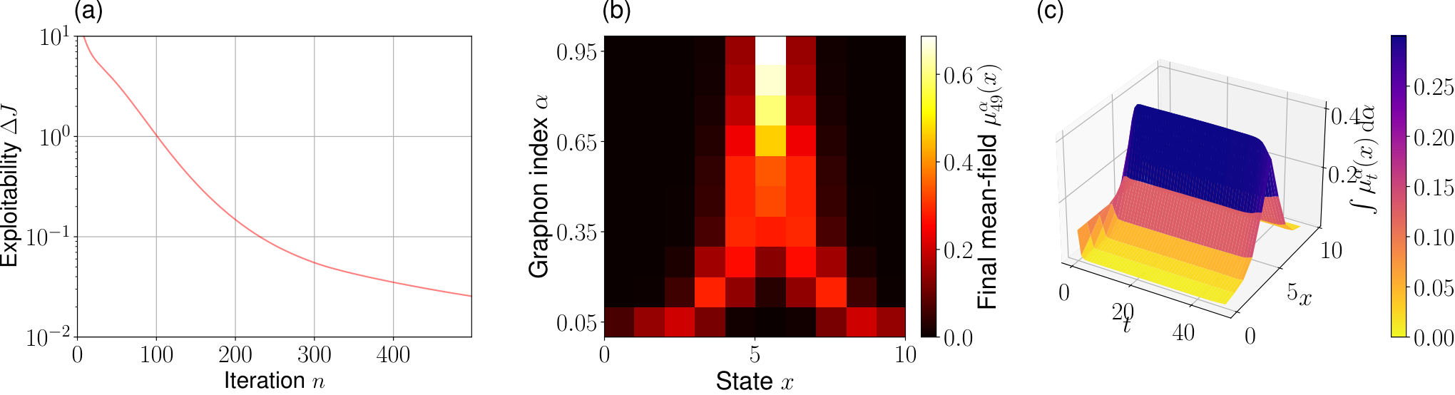
As seen in Figures 2 and 3, the approximate exploitability $\Delta J(\pi)=\int_{\mathcal{I}}\sup_{\pi^{*}\in\Pi}J^{\Psi(\pi)}_{\alpha}(\pi^{*})-J^{\Psi(\pi)}_{\alpha}(\pi)\,\mathrm{d}\alpha$ of a MF policy $\pi$ quantifies the sub-optimality of the obtained equilibrium and quickly converges in the Cyber Security and Beach Bar scenario using OMD. We obtain near-identical results also for the Heterogeneous Cyber Security problem, which are omitted for space reasons. The algorithm converges to an equilibrium where, as expected, the agents with the most connections in the graph attempt to defend at fixed cost, as their expected cost from not defending is higher than for agents with fewer connections. The system quickly runs into an almost time-stationary state, where the costs of defending equilibrate with the expected cost of future infection, see Figure 2. Since we consider a finite-horizon however, the option of defending becomes increasingly unattractive as time runs out. The probability of an agent $\alpha$ being infected at any time shows an interesting behavior: At $\alpha=0$, the probability is quite high due to the great number of connections. As $\alpha$ decreases, so does the probability of being infected at all times. However, as soon as $\alpha$ passes a threshold where defense is no longer individually worth it, the fraction of infected nodes jumps up.

In the heterogeneous case, as seen in Figure 4, we consider an additional class of nodes with partially similar behavior. For very high connectivity $\alpha\to 0$ however, we observe that $\mathrm{Pri}$ nodes will never defend themselves, since for the given problem parameters, the probability of infection will be very high regardless of the defense state. Otherwise, we can observe similar behavior as in the homogeneous case. Perhaps most interesting is the asymmetry between choosing to switch between defended and undefended. When agents are susceptible, some agents will opt to neither switch from defended to undefended, nor vice versa. This stems from the fact that agents switching in state $US$ could likely jump to $UI$ and $DI$, while in state $DS$ likely jumps are $DS$ and $US$, each of which may have different future returns. For the Beach Bar process in Figure 3, we see results similar to the classical ones in Perrin et al., 2020. By giving each agent an incentive to avoid only their direct graphical neighbors, we obtain an equilibrium behavior where agents with many connections will stay further away from the bar, while agents with few connections will not mind many other agents.

Finally, in Figures 5 and 6 for $\rho_{N}=N^{-\beta}$ and sparsity parameter $\beta\in(0,1)$, we observe convergence of the $N$-agent system objective to the MF objective, implying that sufficiently large finite systems are well-approximated by the LPGMFG. In Figure 6, for $\beta$ close to $0$ or $1$, convergence slows down, as by (Borgs et al., 2019, Theorem 2.14) convergence is only guaranteed for $0<\beta<1$. Even though for $\beta=0$, one would get the same model as in Cui and Koeppl, 2022, since the power law graphon is not $[0,1]$-valued, approximation guarantees fail for $\beta=0$ and we observe increasingly slow convergence as we approach zero.

References

- Anahtarci et al., (2020) Anahtarci, B., Kariksiz, C. D., and Saldi, N. (2020). Q-learning in regularized mean-field games. arXiv preprint arXiv:2003.12151.
- Aparicio et al., (2015) Aparicio, S., Villazón-Terrazas, J., and Álvarez, G. (2015). A model for scale-free networks: application to twitter. Entropy, 17(8):5848–5867.
- Arthur, (1994) Arthur, W. B. (1994). Inductive reasoning and bounded rationality. The American Economic Review, 84(2):406–411.
- Aurell et al., (2022) Aurell, A., Carmona, R., Dayanıklı, G., and Laurière, M. (2022). Finite state graphon games with applications to epidemics. Dynamic Games and Applications, pages 1–33.
- Aurell et al., (2021) Aurell, A., Carmona, R., and Lauriere, M. (2021). Stochastic graphon games: II. the linear-quadratic case. arXiv preprint arXiv:2105.12320.
- Avena-Koenigsberger et al., (2018) Avena-Koenigsberger, A., Misic, B., and Sporns, O. (2018). Communication dynamics in complex brain networks. Nature Reviews Neuroscience, 19(1):17–33.
- Bakker et al., (2010) Bakker, L., Hare, W., Khosravi, H., and Ramadanovic, B. (2010). A social network model of investment behaviour in the stock market. Physica A: Statistical Mechanics and its Applications, 389(6):1223–1229.
- Barabási and Albert, (1999) Barabási, A.-L. and Albert, R. (1999). Emergence of scaling in random networks. Science, 286(5439):509–512.
- Barabási et al., (1999) Barabási, A.-L., Albert, R., and Jeong, H. (1999). Mean-field theory for scale-free random networks. Physica A: Statistical Mechanics and its Applications, 272(1-2):173–187.
- Bayraktar et al., (2020) Bayraktar, E., Chakraborty, S., and Wu, R. (2020). Graphon mean field systems. arXiv preprint arXiv:2003.13180.
- Bertsekas, (2019) Bertsekas, D. (2019). Reinforcement learning and optimal control. Athena Scientific.
- Bian et al., (2016) Bian, Y.-t., Xu, L., and Li, J.-s. (2016). Evolving dynamics of trading behavior based on coordination game in complex networks. Physica A: Statistical Mechanics and its Applications, 449:281–290.
- Bollobás et al., (2007) Bollobás, B., Janson, S., and Riordan, O. (2007). The phase transition in inhomogeneous random graphs. Random Structures & Algorithms, 31(1):3–122.
- Borgs et al., (2018) Borgs, C., Chayes, J., Cohn, H., and Zhao, Y. (2018). An Lp theory of sparse graph convergence II: Ld convergence, quotients and right convergence. The Annals of Probability, 46(1):337–396.
- Borgs et al., (2019) Borgs, C., Chayes, J., Cohn, H., and Zhao, Y. (2019). An Lp theory of sparse graph convergence I: Limits, sparse random graph models, and power law distributions. Transactions of the American Mathematical Society, 372(5):3019–3062.
- Borgs et al., (2011) Borgs, C., Chayes, J., Lovász, L., Sós, V., and Vesztergombi, K. (2011). Limits of randomly grown graph sequences. European Journal of Combinatorics, 32(7):985–999.
- Bullmore and Sporns, (2009) Bullmore, E. and Sporns, O. (2009). Complex brain networks: graph theoretical analysis of structural and functional systems. Nature Reviews Neuroscience, 10(3):186–198.
- Bullmore and Sporns, (2012) Bullmore, E. and Sporns, O. (2012). The economy of brain network organization. Nature Reviews Neuroscience, 13(5):336–349.
- Caines and Huang, (2019) Caines, P. E. and Huang, M. (2019). Graphon mean field games and the GMFG equations: -Nash equilibria. In 2019 IEEE 58th Conference on Decision and Control (CDC), pages 286–292. IEEE.
- Canese et al., (2021) Canese, L., Cardarilli, G. C., Di Nunzio, L., Fazzolari, R., Giardino, D., Re, M., and Spanò, S. (2021). Multi-agent reinforcement learning: A review of challenges and applications. Applied Sciences, 11(11):4948.
- Cardaliaguet and Hadikhanloo, (2017) Cardaliaguet, P. and Hadikhanloo, S. (2017). Learning in mean field games: the fictitious play. ESAIM: Control, Optimisation and Calculus of Variations, 23(2):569–591.
- Carmona, (2004) Carmona, G. (2004). Nash equilibria of games with a continuum of players.
- Carmona et al., (2022) Carmona, R., Cooney, D. B., Graves, C. V., and Lauriere, M. (2022). Stochastic graphon games: I. the static case. Mathematics of Operations Research, 47(1):750–778.
- (24) Carmona, R. and Delarue, F. (2018a). Probabilistic Theory of Mean Field Games with Applications I: Mean Field FBSDEs, Control, and Games, volume 83. Springer.
- (25) Carmona, R. and Delarue, F. (2018b). Probabilistic Theory of Mean Field Games with Applications II: Mean Field Games with Common Noise and Master Equations. Probability Theory and Stochastic Modelling. Springer International Publishing.
- Carmona et al., (2015) Carmona, R., Fouque, J.-P., and Sun, L.-H. (2015). Mean field games and systemic risk. Communications in Mathematical Sciences, 13(4):911–933.
- Carmona et al., (2019) Carmona, R., Laurière, M., and Tan, Z. (2019). Model-free mean-field reinforcement learning: mean-field mdp and mean-field q-learning. arXiv preprint arXiv:1910.12802.
- Carmona and Zhu, (2016) Carmona, R. and Zhu, X. (2016). A probabilistic approach to mean field games with major and minor players. The Annals of Applied Probability, 26(3):1535–1580.
- Castiglione et al., (2014) Castiglione, A., Gribaudo, M., Iacono, M., and Palmieri, F. (2014). Exploiting mean field analysis to model performances of big data architectures. Future Generation Computer Systems, 37:203–211.
- Choutri and Djehiche, (2019) Choutri, S. E. and Djehiche, B. (2019). Mean-field risk sensitive control and zero-sum games for markov chains. Bulletin des Sciences Mathématiques, 152:1–39.
- Choutri et al., (2019) Choutri, S. E., Djehiche, B., and Tembine, H. (2019). Optimal control and zero-sum games for markov chains of mean-field type. Mathematical Control & Related Fields, 9(3):571.
- Concas et al., (2007) Concas, G., Marchesi, M., Pinna, S., and Serra, N. (2007). Power-laws in a large object-oriented software system. IEEE Transactions on Software Engineering, 33(10):687–708.
- Conitzer and Sandholm, (2008) Conitzer, V. and Sandholm, T. (2008). New complexity results about Nash equilibria. Games and Economic Behavior, 63(2):621–641.
- Cui and Koeppl, (2021) Cui, K. and Koeppl, H. (2021). Approximately solving mean field games via entropy-regularized deep reinforcement learning. In International Conference on Artificial Intelligence and Statistics, pages 1909–1917. PMLR.
- Cui and Koeppl, (2022) Cui, K. and Koeppl, H. (2022). Learning graphon mean field games and approximate Nash equilibria. In International Conference on Learning Representations.
- Cui et al., (2022) Cui, K., Li, M., Fabian, C., and Koeppl, H. (2022). Scalable task-driven robotic swarm control via collision avoidance and learning mean-field control. arXiv preprint arXiv:2209.07420.
- Delarue and Vasileiadis, (2021) Delarue, F. and Vasileiadis, A. (2021). Exploration noise for learning linear-quadratic mean field games. arXiv preprint arXiv:2107.00839.
- D’Arcangelis and Rotundo, (2016) D’Arcangelis, A. M. and Rotundo, G. (2016). Complex networks in finance. In Complex Networks and Dynamics, pages 209–235. Springer.
- Elamvazhuthi and Berman, (2019) Elamvazhuthi, K. and Berman, S. (2019). Mean-field models in swarm robotics: A survey. Bioinspiration & Biomimetics, 15(1):015001.
- (40) Elie, R., Ichiba, T., and Laurière, M. (2020a). Large banking systems with default and recovery: A mean field game model. arXiv preprint arXiv:2001.10206.
- (41) Elie, R., Perolat, J., Laurière, M., Geist, M., and Pietquin, O. (2020b). On the convergence of model free learning in mean field games. In Proceedings of the AAAI Conference on Artificial Intelligence, volume 34, pages 7143–7150.
- Farago et al., (2002) Farago, J., Greenwald, A., and Hall, K. (2002). Fair and efficient solutions to the santa fe bar problem. In Grace Hopper Celebration of Women in Computing. Citeseer.
- Firoozi et al., (2020) Firoozi, D., Jaimungal, S., and Caines, P. E. (2020). Convex analysis for lqg systems with applications to major–minor lqg mean–field game systems. Systems & Control Letters, 142:104734.
- Gao and Caines, (2017) Gao, S. and Caines, P. E. (2017). The control of arbitrary size networks of linear systems via graphon limits: An initial investigation. In 2017 IEEE 56th Annual Conference on Decision and Control (CDC), pages 1052–1057. IEEE.
- Gao et al., (2021) Gao, S., Tchuendom, R. F., and Caines, P. E. (2021). Linear quadratic graphon field games. Communications in Information and Systems, 21(3):341–369.
- Gkogkas and Kuehn, (2022) Gkogkas, M. A. and Kuehn, C. (2022). Graphop mean-field limits for kuramoto-type models. SIAM Journal on Applied Dynamical Systems, 21(1):248–283.
- Guo et al., (2019) Guo, X., Hu, A., Xu, R., and Zhang, J. (2019). Learning mean-field games. In Advances in Neural Information Processing Systems, pages 4966–4976.
- Guo et al., (2020) Guo, X., Hu, A., Xu, R., and Zhang, J. (2020). A general framework for learning mean-field games. arXiv preprint arXiv:2003.06069.
- Guo et al., (2022) Guo, X., Xu, R., and Zariphopoulou, T. (2022). Entropy regularization for mean field games with learning. Mathematics of Operations Research.
- Hadikhanloo, (2017) Hadikhanloo, S. (2017). Learning in anonymous nonatomic games with applications to first-order mean field games. arXiv preprint arXiv:1704.00378.
- Hadikhanloo and Silva, (2019) Hadikhanloo, S. and Silva, F. J. (2019). Finite mean field games: fictitious play and convergence to a first order continuous mean field game. Journal de Mathématiques Pures et Appliquées, 132:369–397.
- Huang et al., (2020) Huang, K., Di, X., Du, Q., and Chen, X. (2020). A game-theoretic framework for autonomous vehicles velocity control: Bridging microscopic differential games and macroscopic mean field games. Discrete & Continuous Dynamical Systems-B, 25(12):4869.
- Huang et al., (2006) Huang, M., Malhamé, R. P., and Caines, P. E. (2006). Large population stochastic dynamic games: closed-loop mckean-vlasov systems and the Nash certainty equivalence principle. Communications in Information & Systems, 6(3):221–252.
- Khalil, (2002) Khalil, H. (2002). Nonlinear Systems. Pearson Education. Prentice Hall.
- Kolokoltsov and Bensoussan, (2016) Kolokoltsov, V. N. and Bensoussan, A. (2016). Mean-field-game model for botnet defense in cyber-security. Applied Mathematics & Optimization, 74(3):669–692.
- Kolokoltsov and Malafeyev, (2018) Kolokoltsov, V. N. and Malafeyev, O. A. (2018). Corruption and botnet defense: a mean field game approach. International Journal of Game Theory, 47(3):977–999.
- Lacker and Soret, (2022) Lacker, D. and Soret, A. (2022). A case study on stochastic games on large graphs in mean field and sparse regimes. Mathematics of Operations Research, 47(2):1530–1565.
- Lasry and Lions, (2007) Lasry, J.-M. and Lions, P.-L. (2007). Mean field games. Japanese Journal of Mathematics, 2(1):229–260.
- Laurière et al., (2022) Laurière, M., Perrin, S., Girgin, S., Muller, P., Jain, A., Cabannes, T., Piliouras, G., Pérolat, J., Élie, R., Pietquin, O., et al. (2022). Scalable deep reinforcement learning algorithms for mean field games. arXiv preprint arXiv:2203.11973.
- Li et al., (2019) Li, M., Qin, Z., Jiao, Y., Yang, Y., Wang, J., Wang, C., Wu, G., and Ye, J. (2019). Efficient ridesharing order dispatching with mean field multi-agent reinforcement learning. In The world wide web conference, pages 983–994.
- Louridas et al., (2008) Louridas, P., Spinellis, D., and Vlachos, V. (2008). Power laws in software. ACM Transactions on Software Engineering and Methodology (TOSEM), 18(1):1–26.
- Lovász, (2012) Lovász, L. (2012). Large networks and graph limits, volume 60. American Mathematical Soc.
- Mertikopoulos et al., (2018) Mertikopoulos, P., Papadimitriou, C., and Piliouras, G. (2018). Cycles in adversarial regularized learning. In Proceedings of the Twenty-Ninth Annual ACM-SIAM Symposium on Discrete Algorithms, pages 2703–2717. SIAM.
- Mguni et al., (2018) Mguni, D., Jennings, J., and de Cote, E. M. (2018). Decentralised learning in systems with many, many strategic agents. Thirty-Second AAAI Conference on Artificial Intelligence.
- Mondal et al., (2021) Mondal, W. U., Agarwal, M., Aggarwal, V., and Ukkusuri, S. V. (2021). On the approximation of cooperative heterogeneous multi-agent reinforcement learning (MARL) using mean field control (MFC). arXiv preprint arXiv:2109.04024.
- Newman, (2005) Newman, M. (2005). Power laws, pareto distributions and zipf’s law. Contemporary Physics, 46(5):323–351.
- Newman, (2018) Newman, M. (2018). Networks. Oxford University Press.
- Newman, (2002) Newman, M. E. (2002). Spread of epidemic disease on networks. Physical Review E, 66(1):016128.
- Nosonovsky and Roy, (2020) Nosonovsky, M. and Roy, P. (2020). Scaling in colloidal and biological networks. Entropy, 22(6):622.
- Nourian and Caines, (2013) Nourian, M. and Caines, P. E. (2013). -Nash mean field game theory for nonlinear stochastic dynamical systems with major and minor agents. SIAM Journal on Control and Optimization, 51(4):3302–3331.
- Orabona et al., (2015) Orabona, F., Crammer, K., and Cesa-Bianchi, N. (2015). A generalized online mirror descent with applications to classification and regression. Machine Learning, 99(3):411–435.
- Papadimitriou, (2001) Papadimitriou, C. (2001). Algorithms, games, and the internet. In Proceedings of the Thirty-Third Annual ACM Symposium on Theory of Computing, pages 749–753.
- Papadimitriou, (2007) Papadimitriou, C. H. (2007). The complexity of finding Nash equilibria. Algorithmic Game Theory, 2:30.
- Pastor-Satorras et al., (2015) Pastor-Satorras, R., Castellano, C., Van Mieghem, P., and Vespignani, A. (2015). Epidemic processes in complex networks. Reviews of Modern Physics, 87(3):925.
- Perolat et al., (2021) Perolat, J., Perrin, S., Elie, R., Laurière, M., Piliouras, G., Geist, M., Tuyls, K., and Pietquin, O. (2021). Scaling up mean field games with online mirror descent. arXiv preprint arXiv:2103.00623.
- (76) Perrin, S., Laurière, M., Pérolat, J., Élie, R., Geist, M., and Pietquin, O. (2021a). Generalization in mean field games by learning master policies. arXiv preprint arXiv:2109.09717.
- (77) Perrin, S., Laurière, M., Pérolat, J., Geist, M., Élie, R., and Pietquin, O. (2021b). Mean field games flock! the reinforcement learning way. In Proceedings of the Thirtieth International Joint Conference on Artificial Intelligence, IJCAI-21, pages 356–362. International Joint Conferences on Artificial Intelligence Organization. Main Track.
- Perrin et al., (2020) Perrin, S., Pérolat, J., Laurière, M., Geist, M., Elie, R., and Pietquin, O. (2020). Fictitious play for mean field games: Continuous time analysis and applications. Advances in Neural Information Processing Systems, 33:13199–13213.
- Qu et al., (2020) Qu, G., Wierman, A., and Li, N. (2020). Scalable reinforcement learning of localized policies for multi-agent networked systems. In Learning for Dynamics and Control, pages 256–266. PMLR.
- Rozemberczki et al., (2019) Rozemberczki, B., Davies, R., Sarkar, R., and Sutton, C. (2019). GEMSEC: Graph embedding with self clustering. In 2019 IEEE/ACM International Conference on Advances in Social Networks Analysis and Mining (ASONAM), pages 65–72. IEEE Computer Society.
- Saldi et al., (2018) Saldi, N., Basar, T., and Raginsky, M. (2018). Markov–Nash equilibria in mean-field games with discounted cost. SIAM Journal on Control and Optimization, 56(6):4256–4287.
- Sporns, (2022) Sporns, O. (2022). Structure and function of complex brain networks. Dialogues in Clinical Neuroscience.
- Srebro et al., (2011) Srebro, N., Sridharan, K., and Tewari, A. (2011). On the universality of online mirror descent. Advances in Neural Information Processing Systems, 24.
- Subramanian and Mahajan, (2019) Subramanian, J. and Mahajan, A. (2019). Reinforcement learning in stationary mean-field games. In Proceedings of the 18th International Conference on Autonomous Agents and MultiAgent Systems, pages 251–259.
- Tangpi and Zhou, (2022) Tangpi, L. and Zhou, X. (2022). Optimal investment in a large population of competitive and heterogeneous agents. arXiv preprint arXiv:2202.11314.
- Wheeldon and Counsell, (2003) Wheeldon, R. and Counsell, S. (2003). Power law distributions in class relationships. In Proceedings Third IEEE International Workshop on Source Code Analysis and Manipulation, pages 45–54. IEEE.
- Yang et al., (2018) Yang, J., Ye, X., Trivedi, R., Xu, H., and Zha, H. (2018). Learning deep mean field games for modeling large population behavior. In International Conference on Learning Representations.
- Yang and Wang, (2020) Yang, Y. and Wang, J. (2020). An overview of multi-agent reinforcement learning from game theoretical perspective. arXiv preprint arXiv:2011.00583.
- Zhang et al., (2021) Zhang, K., Yang, Z., and Başar, T. (2021). Multi-agent reinforcement learning: A selective overview of theories and algorithms. Handbook of Reinforcement Learning and Control, pages 321–384.
SUPPLEMENTARY MATERIAL
The following pages provide additional information and proofs for the statements in the main part of the paper "Learning Sparse Graphon Mean Field Games". In the sections A to D we give the proofs of Theorems 2 and 3. Subsequently, sections E to H contain the proofs of Theorem 4 and the necessary intermediate results. Furthermore, the sections I to M include the details of the learning methods as well as the proofs for the theoretical convergence guarantee (Theorem 5) of the OMD algorithm. We provide a derivation of the cutoff power law graphon in section N and conclude the supplementary materials with the problem details for our examples in section O.
Appendix A OVERVIEW
In this section we collect intermediate results and auxiliary definitions that help to prove Theorems 2 and 3. Proofs which require an extensive argumentation are deferred to the subsequent paragraphs. First, we define the -neighborhood map of an agent by
and similarly the empirical -neighborhood map by
Here, we point out that holds for the MF system and holds for the finite model. For the following proofs, we require the concept of an ensemble transition kernel operator which is defined by
where is a graphon, , and . This definition especially implies the useful property . For convenience, we also introduce the notation
To prove Theorem 3, we have to establish the following result which is proven in a subsequent section. Note that this Lemma 2 is not required in the standard graphon theory but becomes necessary for our graphon approach. Specifically, the proof of Lemma 3 will include functions of the form for which a result like the one given by Theorem 2 is required. However, the factor introduced as part of the graphon approach makes it impossible to bound functions such as uniformly over all because for sparse graphs approaches infinity as approaches infinity. Therefore, Theorem 2 is not applicable in this case which makes a new statement, i.e. Lemma 2, necessary. Put differently, the formulation and proof of Lemma 2 is a new mathematical contribution of our work.
Lemma 2.
Let be a sequence of positive real numbers such that and and let be some sequence of sets with . Then, we consider a sequence of measurable functions where for all we have if and otherwise. Consider Lipschitz continuous up to a finite number of discontinuities , with associated mean field ensemble . Under Assumption 1 and the -agent policy with , , , we have