Observation of coherent oscillations in association of dimers from a thermal gas of ultracold atoms.
Abstract
We report the observation of coherent oscillations in conversion efficiency of weakly-bound dimers formed from a thermal gas of ultracold atoms. Finite thermal energy of the gas causes loss of coherence when a broad continuum is resonantly coupled to a discrete bound state. Restoration of the coherence can be achieved through non-adiabatic transitions of the dressed molecular energy level that are induced by a strong modulation pulse with fast envelope dynamics. Conditions to observe coherent oscillations are verified, and control of their properties is demonstrated. The main experimental findings are supported by theoretical modeling and numerical calculations. The observed results may lead to a renewed interest in general studies of a discrete energy level coupled to a broadband continuum when the properties of both are fully controlled.
When coupling between a discrete energy level and a broad continuum is introduced, dynamics is expected to be fully incoherent due to vanishingly short coherent memory of the latter. Numerous quantum electrodynamics systems such as spontaneous emission of an excited atom, photoionization of an atom and photodissociation of molecules are all fit within the framework of this general scheme CohenTannoudji. A similar system can be realized with ultracold atoms in the vicinity of collisional resonances which are characterized by the existence of a weakly bound dimer state. An original experimental technique to probe this state was demonstrated in Ref. Thompson05 which consisted of association of dimers from a thermal gas of atoms by modulating the magnetic field bias at a frequency that matches the binding energy. Surprisingly, coherent Rabi-type oscillations in the dimers conversion efficiency has been reported and remained unexplained since then despite the number of theoretical approaches devoted to the subject Hanna07; Bazak12; Brouard15; Langmack15; Mohapatra15 and despite the straightforward analogy with the mentioned above systems subject to broadband decoherence mechanisms.
A recent theoretical proposal suggests a mechanism that leads to the restoration of coherence in such a system Giannakeas19. Here we carefully explore its conditions and provide the experimental verification. Our studies reveal the crucial importance of fast dynamics initiated by the excitation pulse envelope. The mechanism bares similarities with Stückelberg oscillations demonstrated earlier in multiphoton ionization Jones95 and in Rydberg excitation Bengs22 of atoms. More recently, similar effect has been suggested theoretically also for x-ray ionization by intense femtosecond laser pulses where their steep raise and fall induces dynamic interference in the photoionization spectra Demekhin12a; toyotanjp2015; Baghery17; Ning18; com2.

Conversion of ultracold atoms into a weakly bound dimer is executed by modulation of the magnetic field bias with a resonance frequency , as shown in Fig. 1(a). To illustrate the physical mechanism behind the coherent oscillations in the molecule conversion efficiency, the induced interaction dynamics is represented in Fig. 1(b) as a dressed state energy level in the rotating wave approximation. Before the modulation pulse is switched on, the dressed energy level is degenerate with the thermal continuum. When the modulation strength grows, experiences repulsion from the continuum and is pushed down to lower energies. Ultimately, at strong enough modulation crosses the dissociation threshold and opens a gap with the continuum (, see Fig. 1(b)). If the dynamical changes () of the dressed level are fast compared to timescale set by the thermal energy () the nonadiabatic coupling creates an effective beam-splitter each time the threshold is passed and forms a two-path interferometer for a wave function to either make a dimer or remain in an unbound state (see Fig. 1(b)). As was demonstrated in Ref. Giannakeas19 such an interferometer should be robust against thermal averaging and, as we show here, it is responsible for the observed coherent oscillations.
Our study settles a long-term quest for a deeper understanding of an experimental technique routinely used for nearly two decades in many species and mixtures such as homo- Papp06; Lange09; Gross11; Dyke13 and hetero-nuclear atomic systems Gaebler07; Weber08; Wang15 and in strongly magnetic atoms Frisch15; Ye22. Revealing a non-adiabatic effect related to the fast dynamics of the modulation pulse envelope provides an old problem with a fresh perspective and novel and unexpected relations with other systems such as, for example, photoionization with intense femtosecond laser pulses Demekhin12a; toyotanjp2015; Baghery17; Ning18; com2. In this context, our work complements and enhances a recently established quantum simulator of ultrafast phenomena with ultracold atoms Senaratne18. Even in a broader context, our results pave the way for studies of a discrete energy level coupled strongly to a broadband continuum in a well controlled environment provided by ultracold atoms in which both the energy level and the continuum properties can be adjusted.
The experiment is performed in a thermal gas of 7Li atoms, polarized in the state and evaporatively cooled to a temperature of K in a crossed-beam optical trap Gross08. Feshbach dimers are associated in the vicinity of the G -wave Feshbach resonance by means of a magnetic field modulation at a frequency of MHz. The latter is in resonance with the dimer’s binding energy when the magnetic field bias is set to G, which corresponds to the scattering length Gross11; Julienne14. The modulation is applied by 2 auxiliary coils on both sides of the vacuum chamber, aligned with the magnetic field bias.
In the first set of experiments we explore the effect of large modulation amplitudes on the dimer binding energy. Up to a second order in perturbation theory the dimer energy (averaged over a modulation period) is expressed as a dressed state supMat:
| (1) |
where is the dimer binding energy for vanishing modulation strength in the universal limit, and are the corresponding scattering length and magnetic field, and are the width and location of the Feshbach resonance, and corrects for the finite range of the potential and the resonance strength. When the modulation frequency satisfies the resonance condition, i.e. , dimers are formed most efficiently Thompson05. Thus, characterizing the optimal dimer conversion efficiency as a function of modulation strength and using Eq. (1) allows for accurate calibration of at the position of atoms. This information is important to verify the first condition to observe Stückelberg oscillations.
In the experiment the modulation frequency is fixed and we scan the magnetic field bias to find the resonance response in dimer association. Recasting Eq. (1) in this language we get:
| (2) |
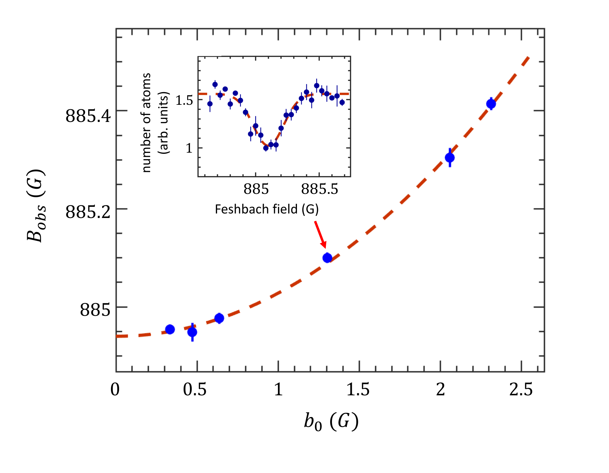
For each value of we scan the magnetic field bias and measure the number of remaining atoms in the trap after a short waiting time during which the molecules decay from the trap due to inelastic collisions (see Fig. 2 (inset)). The pulse duration is varied from s to s to keep the loss contrast (, where is the background and the minimal number of atoms) roughly constant and . The resulting loss resonance is fitted with a Gaussian profile and the center value is extracted. In Fig. 2 is shown as a function of revealing that a maximal shift of mG can be readily obtained with a modulation amplitude as large as G at the position of atoms supMat. This corresponds to an energy shift of kHz which surpasses the thermal energy by almost one order of magnitude and satisfies the condition to observe Stückelberg oscillations. Note that having this large energy margin is essential for the success of the experimental demonstration as will be clarified below.
Consider next the main experimental protocol used for the observation of the Stückelberg oscillations. The modulation coils are part of a resonant RLC circuit to maximize the available modulation amplitude. This results into a time-dependent magnetic field of the following form:
| (3) |
where is the pulse envelope described by the relation:
| (4) |
where is the pulse duration, is the amplitude at the moment the pulse is switched off and are the rise and fall times of the pulse envelope. Fig. 3 shows the pulse’s envelope as measured by a pick-up antenna. By fitting it to Eq. (4) the rise and fall times are extracted to be s and s. Note that the typical timescale of the system attributed to the finite thermal energy is longer than the envelope’s dynamics (s ) satisfying the non-adiabaticity criterion (see Fig. 1(b)). The dressed energy level dynamics is now described by Eq. (1) where is substituted with .

Before the modulation pulse is turned on, a bias field is applied, such that . As the pulse is turned on is shifted to lower values, and when the pulse is turned off the energy level goes back to its initial value. We explore three different scenarios illustrated in Fig. 4(a). They differ from each other only by the applied bias field (), so that although the initial energies are different, the modulation amplitude remains the same for all scenarios. This approach assures minimal changes in the experimental conditions which is less so if, for example, the pulse intensity is varied instead. To keep the validity of nonadiabaticity in all scenarios we start above the threshold with at least (see Fig. 4(a)). This forces the dressed dimer energy level to pass the majority of populated continuum rapidly, and is especially relevant to avoid the problematic long tail of weak modulation when the pulse is switched off (see the red dashed tail in Fig. 3).
For the scenarios (ii) and (iii) we expect Stückelberg oscillations in dimer conversion efficiency. When the pulse amplitude starts to grow the initial non-adiabatic passage of the dressed energy level through the continuum imitates the entrance beam splitter of an interferometer at which the initial wave function splits between the free atoms and the bound state pathways. As the pulse amplitude continues to grow, the two paths decouple and accumulate a dynamic phase difference according to their energy separation. When the pulse is turned off the dressed dimer level crosses the continuum again, this time imitating the exit beam splitter at which the two pathways of the wave function recombine. The resulting interference is measured through counting the number of free atoms as a function of pulse duration (see Fig. 3). Note that the population of the dimer state is hidden in the dark because, prior to detection, the magnetic field bias is shifted to deepen the dimer binding energy to MHz. Thus, the bound state remains decoupled from the weak, on-resonance detection light. In the first scenario (i) of Fig. 4(a) the dynamics is mostly adiabatic for energies near which efficiently eliminates the entrance beam splitter. Although the exit beam splitter is still created by the sharp end of the pulse, Stückelberg oscillations are not expected in this case.

The experimental results and the corresponding numerical calculations based on the integration of the time dependent Schrödinger equation are shown in Fig. 4(b,c,d) and (e,f,g) respectively. Each data point is an average of runs, and the error bars signify the standard deviation. All measurements are performed with the maximal modulation amplitude of G. The numerics are done according to prescriptions of Ref. Giannakeas19 with parameters suitable for our experimental realization and they show qualitative agreement with the measurements (for details see supMat). Quantitative discrepancies are discussed at the end of this section.
In case (i), shown in Fig. 4(b), the bias field is set to G (see Fig. 2) and the dressed level becomes resonant with the continuum only when the pulse amplitude reaches its maximum. The interferometric sequence is not realized in this case which can be identified in the monotonic decrease in number of atoms as a function of pulse duration . For s and s, the signal agrees with static saturation. In the former case the pulse amplitude is still weak and the modulation frequency is off-resonance as can be seen in Fig. 4(a), keeping the production efficiency low. The latter is obtained when the rates of association and dissociation of dimers due to on-resonance modulation become equal. Similar behavior can be identified in the numerical calculations shown in Fig. 4(e).
In case (ii), shown in Fig. 4(c), the bias field is set to G. Since now the initial dimer energy is lower, the dressed dimer level crosses the threshold and reaches a separation with the continuum (Fig. 4(a)). The oscillations are visible here with two minima and two maxima that can be readily identified, and they agree with a frequency of kHz supported by the numerical calculations shown in Fig. 4(f). At longer times the oscillations wash out in both experiment and theory due to the broadband continuum Giannakeas19.
Case (iii) is shown in Fig. 4(d) for which the bias field is set to G. As the dressed dimer energy opens a larger gap with the continuum, a faster oscillation frequency is observed. Also here two minima and two maxima can be identified and their frequency agrees with kHz. Fig. 4(g) shows the corresponding numerical calculations and confirms a faster oscillation frequency. Note, however, that the frequency is not constant. Close examination of both experimental and theoretical curves shows that the short time dynamics is somewhat slower. This is because for the pulse amplitude does not reach its maximal value and the opened gap is therefore smaller.
Although numerical calculations qualitatively agree with the experimental measurements, quantitative discrepancies are visible. The largest discrepancy can be associated with the signals’ contrasts. For example, for incoherent dimer production the theory underestimates the production efficiency by about a factor of two. It can be partially compensated by the fact that the numerical calculations neglect inelastic losses of dimers. While this assumption is correct for all pulse durations used here, in the experiment more time passes between the end of the pulse and the detection during which the majority of dimers are lost. As the dominant loss mechanism involves inelastic collisions between a dimer and a free atom, the measured number of atoms should be smaller by a factor of . Although in this case the agreement would improve, for other sets of measurements the oscillation contrast in the numerical calculations are larger by a factor of (for the first oscillation) and the inclusion of losses will only increase this discrepancy.
We believe that the main disagreement comes from the fact that the numerical calculations are performed with a zero-range model where the universal dimer energies are matched with those obtained from the experimental measurements. Although we work with the scattering length an order of magnitude larger than the van der Waals length of the interatomic potential, the details of the true potential are already responsible for deviation of the binding energy from the universal formula Gross11; supMat. Thus, these details play a role in dimer association especially for short pulse durations (s) for which the bandwidth is comparable to the energy gap between the dressed state and the continuum threshold. Note also that Feshbach resonances in 7Li are all narrow in character Julienne14 which makes a single channel approach less reliable.
In conclusion, a robust coherent phenomenon in the conversion efficiency of Feshbach dimers formed from a thermal gas of ultracold atoms has been experimentally demonstrated and compared with theory. Our proof of concept studies can be improved in many ways. Access to lower temperatures, limited by technical reasons, should improve the contrast of oscillations and allow the study of decoherence rates in the system. This, in turn, opens the way to extend the system to more complex scenarios and to address questions regarding the environment influence on the observed coherent phenomenon. If the density is increased elastic and inelastic collisions between the superposition state constituents might set in and cause collisional broadening or narrowing which can be revealed via measuring decoherence rates as a function of density. Such adjustability of the continuum is an excellent example for the control the platform of ultracold atoms can provide for the system under study.
This research was supported in part by the Israel Science Foundation (Grant No. 1543/20) and by a grant from the United States-Israel Binational Science Foundation (NSF-BSF Grant 2019795), Jerusalem, Israel, and the United States National Science Foundation (NSF Awards 1912350 and 2207977).
References
- (1) Claude Cohen-Tannoudji, Jacques Dupont-Roc, and Gilbert Grynberg. Atom-Photon Interactions: Basic Process and Applications. Wiley-VCH, Weinheim, 2004.
- (2) S. P. Thompson, E. Hodby, and C. E. Wieman. Ultracold molecule production via a resonant oscillating magnetic field. Phys. Rev. Lett., 95:190404, 2005.
- (3) T. M. Hanna, T. Köhler, and K. Burnett. Association of molecules using a resonantly modulated magnetic field. Phys. Rev. A, 75:013606, Jan 2007.
- (4) Betzalel Bazak, Evgeny Liverts, and Nir Barnea. Multipole analysis of radio-frequency reactions in ultracold atoms. Phys. Rev. A, 86:043611, Oct 2012.
- (5) S. Brouard and J. Plata. Feshbach molecule formation through an oscillating magnetic field: subharmonic resonances. J. Phys. B: At. Mol. Opt. Phys., 48:065002, 2015.
- (6) C. Langmack, D. Hudson Smith, and E. Braaten. Association of atoms into universal dimers using an oscillating magnetic field. Phys. Rev. Lett., 114:103002, Mar 2015.
- (7) A. Mohapatra and E. Braaten. Harmonic and subharmonic association of universal dimers in a thermal gas. Phys. Rev. A, 92:013425, Jul 2015.
- (8) P. Giannakeas, L. Khaykovich, J.-M. Rost, and C. H. Greene. Non-adiabatic molecular association in thermal gases driven by radio-frequency pulses. Phys. Rev. Lett., 123:043204, 2019.
- (9) R. R. Jones. Interference effects in the multiphoton ionization of sodium. Phys. Rev. Lett., 74:1091–1094, Feb 1995.
- (10) U. Bengs, S. Patchkovskii, M. Ivanov, and N. Zhavoronkov. All-optical Stückelberg spectroscopy of strongly driven Rydberg states. Phys. Rev. Research, 4:023135, May 2022.
- (11) P. V. Demekhin and L. S. Cederbaum. Dynamic interference of photoelectrons produced by high-frequency laser pulses. Phys. Rev. Lett., 108:253001, Jun 2012.
- (12) K. Toyota, U. Saalmann, and J.-M. Rost. The envelope Hamiltonian for electron interaction with ultrashort pulses. New Journal of Physics, 17(7):073005, jul 2015.
- (13) M. Baghery, U. Saalmann, and J.-M. Rost. Essential conditions for dynamic interference. Phys. Rev. Lett., 118:143202, Apr 2017.
- (14) Q.-C. Ning, U. Saalmann, and J.-M. Rost. Electron dynamics driven by light-pulse derivatives. Phys. Rev. Lett., 120:033203, Jan 2018.
- (15) Note that Demekhin12a contains flaws in the theoretical and numerical results, see Baghery17.
- (16) S. B. Papp and C. E. Wieman. Observation of heteronuclear Feshbach molecules from a gas. Phys. Rev. Lett., 97:180404, Oct 2006.
- (17) A. D. Lange, K. Pilch, A. Prantner, F. Ferlaino, B. Engeser, H.-C. Nägerl, R. Grimm, and C. Chin. Determination of atomic scattering lengths from measurements of molecular binding energies near feshbach resonances. Phys. Rev. A, 79:013622, Jan 2009.
- (18) N. Gross, Z. Shotan, O. Machtey, S.J.J.M.F. Kokkelmans, and L. Khaykovich. Study of Efimov physics in two nuclear-spin sublevels of 7Li. C.R. Physique, 12:4–12, 2011.
- (19) P. Dyke, S. E. Pollack, and R. G. Hulet. Finite-range corrections near a Feshbach resonance and their role in the Efimov effect. Phys. Rev. A, 88:023625, 2013.
- (20) J. P. Gaebler, J. T. Stewart, J. L. Bohn, and D. S. Jin. -wave Feshbach molecules. Phys. Rev. Lett., 98:200403, May 2007.
- (21) C. Weber, G. Barontini, J. Catani, G. Thalhammer, M. Inguscio, and F. Minardi. Association of ultracold double-species bosonic molecules. Phys. Rev. A, 78:061601(R), Dec 2008.
- (22) F. Wang, X. He, X. Li, B. Zhu, J. Chen, and D. Wang. Formation of ultracold NaRb Feshbach molecules. New J. Phys., 17:035003, 2015.
- (23) A. Frisch, M. Mark, K. Aikawa, S. Baier, R. Grimm, A. Petrov, S. Kotochigova, G. Quéméner, M. Lepers, O. Dulieu, and F. Ferlaino. Ultracold dipolar molecules composed of strongly magnetic atoms. Phys. Rev. Lett., 115:203201, Nov 2015.
- (24) Z.-X. Ye, A. Canali, E. Soave, M. Kreyer, Y. Yudkin, C. Ravensbergen, E. Kirilov, and R. Grimm. Observation of low-field Feshbach resonances between and . Phys. Rev. A, 106:043314, Oct 2022.
- (25) R. Senaratne, S. V. Rajagopal, T. Shimasaki, P. E. Dotti, K. M. Fujiwara, K. Singh, Z. A. Geiger, and D. M. Weld. Quantum simulation of ultrafast dynamics using trapped ultracold atoms. Nature Communications, 9(1):2065, 2018.
- (26) N. Gross and L. Khaykovich. All optical production of 7Li Bose-Einstein condensation using Feshbach resonances. Phys. Rev. A, 77:023604, 2008.
- (27) P. S. Julienne and J. M. Hutson. Contrasting the wide Feshbach resonances in 6Li and 7Li. Phys. Rev. A, 89:052715, 2014.
- (28) See Supplemental Material which includes Ref. Chin10 for the experimental details explaining Fig. 2, notes on derivation of Eqs. (1) and (2), likelihood analysis of the data and clarifications on theoretical model.
- (29) C. Chin, R. Grimm, P. Julienne, and E. Tiesinga. Feshbach resonances in ultracold gases. Rev. Mod. Phys., 82:1225, 2010.
Supplemental Material
Experimental Details. In the experiment is measured as a function of current drawn by the RLC circuit from its power supplier. Assuming and fitting the result with Eq. (2) of the main text we extract the conversion coefficient to be G/A. The same coefficient can be directly calculated from the Biot-Savart (BS) law and the known geometry of our current coils which gives G/A. Although the uncertainty on the BS calculation is quite large (due to geometrical uncertainties) the two values are in a very good agreement with each other.
Notes on the Derivation of Eqs. (1) (2). As specified in the main text, we work with 7Li atoms polarized on internal state. The state features two -wave Feshbach resonances shown in Extended Data Fig. 1 Julienne14. We fit this scattering length data with a factorized expression that incudes two poles where :
| (S1) |
In Table 1 the extracted parameters of both resonances are summarized along with differential magnetic moments of the molecular channel with respect to the free-atom continuum , and the effective ranges at the respective resonance positions.
| [G] | [MHz/G] | sres | |||
|---|---|---|---|---|---|
| 893.78 | -237 | -18.7 | -2.66 | 0.49 | |
| 845.3 | 4.64 | -18.7 | -2.66 | 0.0467 |
All experiments are performed within the close vicinity ( G) of the magnetic field G as specified in the main text (see Fig. 2 in the main text). Thus, the following conditions are always well satisfied: and allowing the simplified expression of Eq. (S1):
| (S2) |
where we dropped the index (as only the first resonance is relevant) and the minus sign (as throughout this work) for convenience. Time modulation of the magnetic field (see Eq. (3) in the main text) is transferred to the time modulation of the scattering length as follows:
| (S3) |
where and is satisfied quite well even for the largest modulation strength amplitudes.
The dimer binding energy corresponding to the Feshbach resonance at G is shown in Extended Data Fig. 2. It can easily be observed that in the region of the relevant magnetic field bias the exact dimer is very well approximated by a simple expression: where is the correction to the universal threshold law. The correction is valid only if and it includes two terms: the finite range of the potential and the resonance strength. Its rigorous form is where and is the Gamma function Chin10. The time modulated binding energy is then:
| (S4) |
For vanishing modulation strength (see Eq. S3) we expand this expression in powers of which in our experiment is (see the definition of and Table 1):
| (S5) |
Returning to time dependence we substitute from Eq. S3 in the above expression and expand it in powers of . Keeping in mind that even for largest modulation amplitudes remains of the same order of magnitude as , the expansion is kept up to the same order:
| (S6) |
where we introduced as a binding energy for vanishing modulation strength at the universal threshold law limit (). Taking the time average over an oscillation period and leaving only the leading order non-vanishing correction in , we arrive at Eq. (1) of the main text:
| (S7) |
where is the -independent constant.
As explained in the main text, in the experiment we scan the magnetic field bias rather than rf frequency. It is then more practical to revamp Eq. S7 as a shift in the magnetic field bias. For that we formally represent as a function of (with the help of Eq. S2):
| (S8) |
and substitute it into Eq. S7 which becomes:
| (S9) |
Taking the square root of the last expression and expanding it to the lowest order in the small parameter yields Eq. (2) of the main text. Note that the magnetic field increases with which suits the intuition that the binding energy deepens with the increase of the modulation strength. This is because the modulation frequency is kept constant, so that we need to increase the magnetic field bias to compensate for deepening of the binding energy when increases.
Theoretical Model. In the following additional information is provided on the theoretical model which is employed in Fig. 4 of the main text. In particular we consider two atoms at low collisional energies which interact via a time-dependent Fermi-Huang -wave pseudopotential
| (S10) |
where indicates a time-dependent scattering length which obeys the following relation:
| (S11) |
where denotes the scattering length in the absence of radio-frequency magnetic pulse whose amplitude is . refers to the driving frequency of the pulse and is the pulse’s envelope as depicted in Fig. 3, i.e. of the main text.
To gain a better physical intuition, semi-analytical expression of the transition probability density to the molecular state from an initial continuum one of energy can be derived within the rotating-wave approximation. Namely, Eq. (5) from Ref. Giannakeas19 is adapted for zero-range interactions as in Eq. (S10) yielding the following relations:
| (S12a) | |||
| with | |||
| (S12b) | |||
where is the molecular energy in the absence of the time-dependent field and obeys relation, i.e. . and denotes the depletion of the bound state into the continuum at energies. The time-dependent phase represents the phase accumulation between a continuum state of energy and the intensity shifted dressed molecular state . Furthermore, according to Eq. (S12b) we observe that describes the modification of the dressed molecular state with energy during the pulse. Indeed, the latter induces a shift on the dressed bound state which is proportional to the square of the amplitude of the pulse. This shift for zero-range interactions can be written in a closed form and it obeys the following relation:
| (S13) |
Note that the shift is negative which originates from the level repulsion between the dressed dimer state and the continuum. Recall that the dressed molecular state energetically lies slightly above the threshold; thus there is sufficient density of continuum states that shift the dressed state towards, or even below, the threshold.
Indeed, the intensity shifted dressed molecular state in Eq. (S12b) together with Eq. (S13) provide a qualitative physical insight of Fig. 4(a) shown in the main text. Apart from that, Eq. (S12) addresses also the underlying physics in the case that the strength of the pulse is not sufficiently strong yielding thus a dressed dimer state above the threshold. This scenario is shown on Fig. 4(b) and (e) in the main text, and in the following we demonstrate the necessary conditions which yield a maximal conversion efficiency. For this purpose consider a square-like pulse with FWHM equal to the one used in the experiment and assume that the decay of the dimer state is small, i.e. . Under these considerations the transition amplitude of Eq. (S12) at the end of the square pulse, i.e. at , yields the following expression:
| (S14) |
where is the intensity shifted dimer energy.
For a thermal gas the energy level statistics fulfill a Maxwell-Boltzmann distribution. This implies that there is no preferable initial continuum state, therefore the probability in Eq. (S14) needs to be thermally averaged over an ensemble of continuum states. The thermally averaged yields the fraction of the atoms converted into molecules, i.e conversion efficiency:
| (S15) |
where () is the number of atoms (molecules), is the density of the thermal gas at temperature , and is the Boltzmann constant. is the thermal de Broglie wavelength, i.e. with being the mass of the atoms.
Substituting Eq. (S14) into Eq. (S15) we numerically obtain in the limit of long pulses that the conversion efficiency is maximized when intensity shifted dimer energy is approximately equal to .
| (S16) |
Eq. (S16) demonstrates that for weak radio-frequency pulses the atoms are most efficiently converted into molecules as long as the intensity shifted dimer state and the continuum one with energy are quasi-degenerate, as it is depicted in Fig. 4(a) in the main text.
Likelihood Analysis.

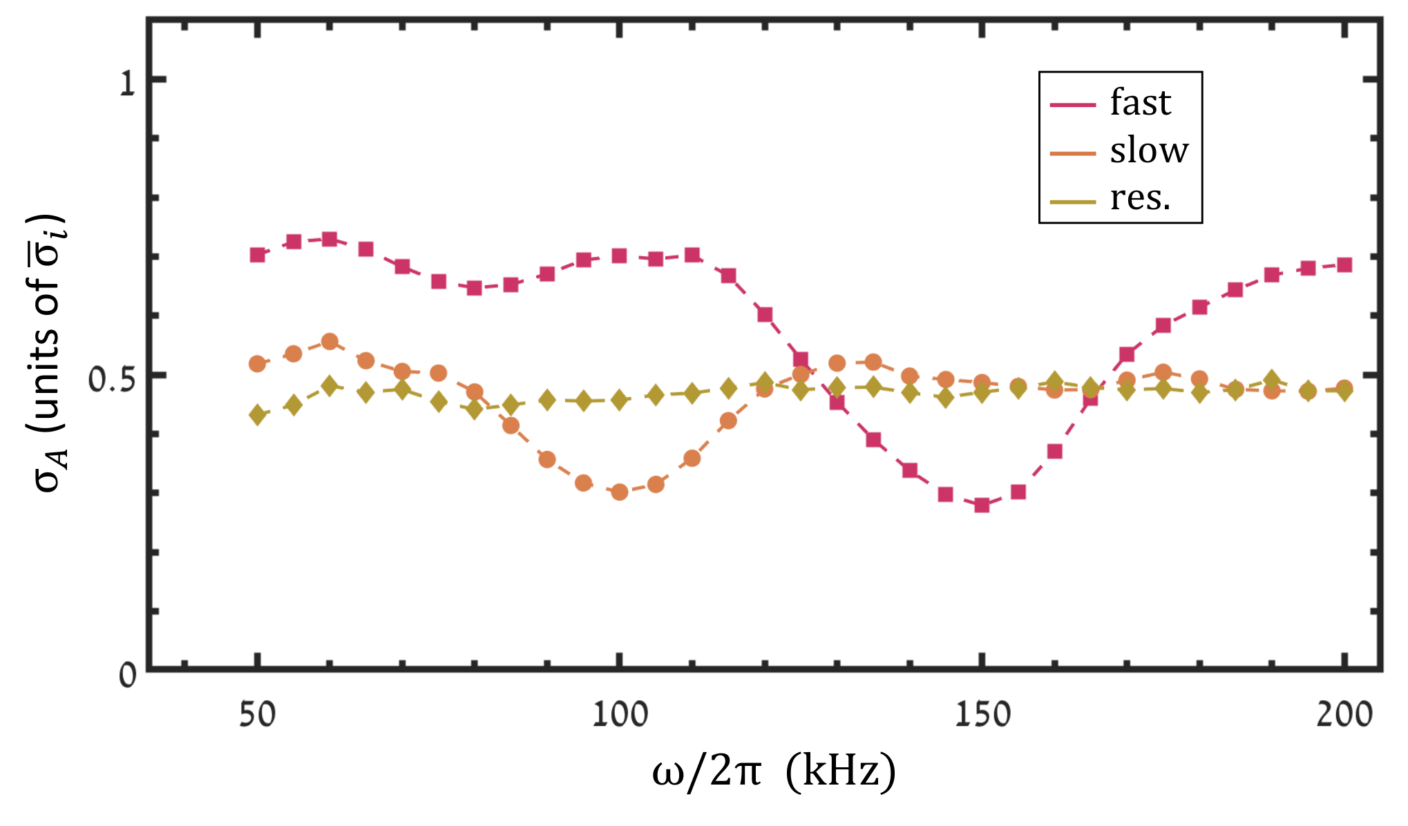
The experimental results shown in this paper suffer from a relatively low signal-to-noise ratio (SNR). Here we analyze the likelihood to obtain a similar sequence of data from a sample of random numbers with the same SNR. Due to a strong decay, there are only two to two and a half oscillations that can be identified in the data. Therefore, our analysis is concentrated only on this region. First, we extract the average standard deviations of noise of these oscillations when the mean value is normalized to one. For two sets of measurements we obtain and for slow and fast oscillations respectively (see Fig. 4 (c),(d) of the main text). We then fit both sequences with keeping and as fitting parameters and scanning kHz. The resulted dependence of the amplitude on is shown in Extended Data Fig. 3(a),(b). The maximal amplitudes for both sequences are, then, and . The best fits corresponding to and are shown in Extended Data Fig. 3(d),(e). To show the significance of the maximal amplitude in the previous analysis we apply it to the experimental data for which we claim no preferred frequency (Fig. 4(b)). However, this data shows strong decay and to remove it we first apply a linear fit to the first s and then subtract it from the data. Next, the analysis proceeds as described above and the results are shown in Extended Data Fig. 3(c),(f). To further emphasize the significance of the preferred frequency, the amplitude error of the fit as a function of frequency for all three cases is shown in Extended Data Fig. 4. The absence of the preferred frequency in the last case is clearly indicated by the absence of a pronounced minimum in the amplitude error. We note that the results shown in Extended Data Fig. 3 are derived from the same two step analysis for all experimental scenarios (i.e. Fig. 4(b),(c),(d)). However, the linear fit to the data of Fig. 4(c),(d) data makes negligible contribution.
We then generate pairs of sequences of random data with and perform fitting of each sequence with the described above fitting procedure. The false positive is counted if for both sequences in a pair and the corresponding frequency of the first falls short of that of the second. This analysis provides us with less than one false positive out of random sequences which corresponds to a statistical significance of of the reported results. This seemingly surprisingly large statistical significance obtained with initially low SNR signals is related to the fact that there are two independent measurements with a meaningful frequency dependence between them. Note that the actual statistical significance of our results is even better because the above analysis excludes the third signal which, for suitable parameters, do not show oscillations baring an additional piece of meaningful information. More fine details of the results that can only strengthen the statistical significance are discussed in the main text.