Occurrence of gap for one-dimensional scalar autonomous functionals with one end point condition
Abstract
Let be a Borel function. We consider the problem
| (P) |
We give an example of a real valued Lagrangian for which the Lavrentiev phenomenon occurs. We state a condition, involving only the behavior of on the graph of two functions, that ensures the non-occurrence of the phenomenon. Our criterium weakens substantially the well-known condition, that is bounded on bounded sets.
LMO, Université Paris-Sud, CNRS, Université Paris–Saclay, 91405 Orsay.
e-mail: Raphael.Cerf@ens.fr
Carlo Mariconda (corresponding author), ORCID , Università degli Studi di Padova, Dipartimento di Matematica “Tullio Levi-Civita”, Via Trieste 63, 35121 Padova, Italy; e-mail: carlo.mariconda@unipd.it†† Mathematics Subject Classification (2010): 49N60
1 Introduction
Consider the basic problem of the Calculus of Variations that consists on minimizing the autonomous integral functional
| (1.1) |
among the absolutely continuous functions on that possibly satisfy some end-point conditions. Here is a Borel function. We are concerned with the question of avoiding the Lavrentiev phenomenon, namely the unpleasant fact that the infimum of among the absolutely continuous functions is strictly less than the one among the Lipschitz functions that share the same end-point conditions. The occurrence of this phenomenon implies the failure of classical numerical analysis methods, e.g., finite elements, if one wishes to compute the infimum of , and represents a discontinuity of with respect to strong convergence in .
Lavrentiev’s phenomenon is considered among experts a matter of non-autonomous Lagrangians, i.e., depending explicitly on the time variable. On one side, a famous example by Manià exhibits the phenomenon when
among the functions that satisfy the end-point conditions (see [4, §4.3]). A more refined construction by Ball and Mizel [2] shows that it may even occur when the Lagrangian is a polynomial in that satisfies Tonelli’s existence conditions (namely superlinearity and convexity in the last variable). On the other side, a celebrated result by Alberti and Serra Cassano [1, Theorem 2.4] asserts that non pathological autonomous Lagrangians do not exhibit the phenomenon. More precisely, there is no Lavrentiev phenomenon if
| (B) |
Notice that Condition (B) forces to be finite on the union and in particular on .
Actually, it has now become clear that the phenomenon is also strictly related to the presence and the number of end-point constraints. For instance, as shown in [4], Manià’s example does not exhibit any more the phenomenon if one considers just the end-point condition . Moreover, it was pointed out in [6] that Condition (B) in [1, Theorem 2.4] is a sufficient condition for the non-occurrence of the phenomenon when one considers just one end-point condition, but not anymore in the case of two end-point conditions. In fact, Alberti provided an example (see [6, Example 3.5]) showing an autonomous Lagrangian with values either 0 or , satisfying (B) such that the functional takes the value on every Lipschitz function satisfying .
Regarding the Lavrentiev phenomenon, the difference between one and two end-point conditions was recently better understood (see [6]). It seems to us of interest to study more thoroughly the conditions that provide the non-occurrence of the phenomenon for problems with one end-point condition. As mentioned above, Condition (B) of [1, Theorem 2.4] does not take into account the geometry of the effective domain of the Lagrangian (i.e., the set where it is finite). We wonder how sharp condition (B) is. Can it be weakened to an assumption involving just the subsets of the effective domain of ? The effort of finding such a condition was carried out in [5] under an additional convexity hypothesis along the radii from the origin on the last variable of the Lagrangian: it is enough in that case that for each , there is such that is bounded on .
In this paper, we consider the case where the Lagrangian is autonomous, , with the initial condition and free end-point condition. We first exhibit a finite, autonomous Lagrangian that violates (B), for which the Lavrentiev phenomenon occurs with just one end-point condition. We introduce the following Condition (R), weaker than (B), that ensures, with no need of any other additional hypothesis, the non-occurrence of the phenomenon:
Condition (R).
There exist two locally Lipschitz functions defined on such that:
and for every bounded interval of ,
The Condition (R) is fulfilled when (B) of [1, Theorem 2.4] holds. Condition (R) has the advantage to require the boundedness of the Lagrangian just on some one-dimensional subsets of its effective domain, without imposing, as (B) does, that contains the union of two-dimensional rectangles.
2 The functional, the gap and the phenomenon
2.1 The functional
For we will denote by the Sobolev space of absolutely continuous functions such that ; is the space of Lipschitz functions on .
We consider an autonomous Borel Lagrangian with non–negative values, possibly infinite. We denote by the unit interval and we define
| (2.1) |
We consider the end–point condition and the problem (P):
| (P) |
2.2 The Lavrentiev gap and phenomenon
We focus our attention on the Lavrentiev gap and phenomenon problems with the prescribed boundary condition . The following definition can be easily adapted to other kinds of boundary conditions.
Definition 2.1 (No gap).
Let . Let be such that . We say that the Lavrentiev gap does not occur at for (P) if there exists a sequence of functions satisfying:
- 1.
for each , the function is Lipschitz and ;
- 2.
(approximation in energy);
- 3.
in (approximation in norm).
We denote by the space of the Lipschitz functions defined on with values in .
Definition 2.2 (No phenomenon).
We say that there is no Lavrentiev phenomenon for if
| (2.2) |
Remark 2.3.
Clearly, the Lavrentiev phenomenon does not occur for once there is no Lavrentiev gap for every such that . Some others kinds of gap are of interest, namely between and for some . They are not considered here since our main result directly prevents the occurrence of the gap between and : the technique of the proof of Theorem 4.1 requires the functions and to be locally Lipschitz.
3 Occurrence of the Lavrentiev gap for (P)
The Lavrentiev phenomenon is often considered a pathology related to non-autonomous Lagrangians. However, the phenomenon may also occur in the autonomous case: an example due to Alberti (see [6, Example 3.5]) exhibits an autonomous Lagrangian that takes the value , satisfies (B), yet the Lavrentiev phenomenon occurs for a problem with two end-point conditions. When Condition (B) fails, the phenomenon may occur in the autonomous case, when one considers just one end-point condition. Consider
| (3.1) |
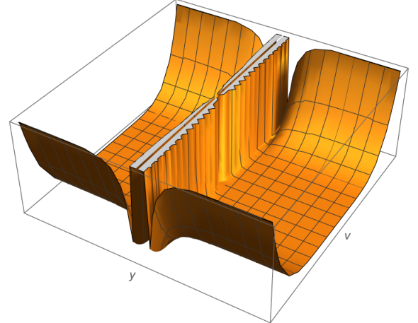
The Lagrangian is a Borel non–negative map. Let . Notice that violates Condition (B) in [1]. Indeed if , then
| (3.2) |
and this implies that, for every , is unbounded on .
Proposition 3.1.
The function is a minimizer for the problem (P) associated to and moreover . The gap occurs at : more precisely, for any such that we have .
Proof.
We have
so that for in . Moreover, we have for all admissible trajectory , therefore
| (3.3) |
Next, let with and assume that . Notice that, since , then is not identically equal to 0. The set being open and non-empty, it is a countable or finite union of non-empty open subintervals of . Hence, there are such that
| (3.4) |
Let . We have
| (3.5) | ||||
Since and is continuous at , then as , so that there exists such that
| (3.6) |
Now, in (3.5), fix . Integrating both terms of (3.6) over , we obtain
| (3.7) |
Inequalities (3.5) and (3.7) together yield
| (3.8) |
Notice that we use the lower bound (3.7) only for the integral over . Jensen’s inequality yields
| (3.9) | ||||
Since and is continuous at , we deduce from (3.9) that
| (3.10) |
Keeping fixed and taking the limit in (3.8) as goes to , we conclude that , contradicting the initial assumption that . ∎
Proposition 3.1 readily implies that the Lavrentiev phenomenon occurs for the problem with one end-point condition given by
| (3.11) |
The recent works [5, 6] have shown that the Lavrentiev phenomenon might be very sensitive to the number of prescribed end-point conditions. In fact, the same argument as above shows that the Lavrentiev phenomenon occurs for the problem with two end-point conditions given by
| (3.12) |
However, in the above example, if we keep only one of the two end-point conditions, the Lavrentiev phenomenon disappears! To see this, we proceed as in [4, §4.3].
4 Non-Occurrence of the Lavrentiev Gap and phenomenon for (P)
4.1 Non-occurrence of the gap
Let be an autonomous Borel Lagrangian with non–negative values, possibly infinite. Let . For a given , we consider the following condition.
Condition (Ry).
There exist two Lipschitz functions defined on such that
Theorem 4.1 (Non-occurrence of the Lavrentiev gap).
Let be such that . Assume that satisfies Condition (Ry). Then there is no Lavrentiev gap for at .
Remark 4.2.
Condition (Ry) weakens Assumption (B) formulated in [1]. Indeed if is bounded on for some , then (Ry) is satisfied with and .
The strategy of the proof is the same as the proof of Alberti and Serra Cassano [1]. Yet it differs at some specific points and it requires also a different construction for the approximating function. In order to facilitate the reading, we have chosen to write the full proof. Another reason is that, as we work with real valued functions, some arguments become simpler than in the –dimensional case. For convenience, we restate a general lemma of integration theory that were proved in [1].
Lemma 4.3.
[1, Lemma 2.6] Let be a Lebesgue measurable function and let be a sequence of measurable subsets of such that as . Then
We will need the following variation of [1, Lemma 2.7]. Compared with the original version we do not need here that the functions are Lipschitz nor that are bounded from below on , and the conclusion is weaker.
Lemma 4.4.
Let , , be a sequence of absolutely continuous functions with a.e. on and be a sequence of measurable sets of such that:
- 1.
For some , a.e. in ;
- 2.
as for every .
Then, for every ,
| (4.1) |
Proof.
Let be a sequence of smooth functions such that in . We write
| (4.2) |
Of course, in and the dominated convergence theorem, for each fixed, implies that as . It remains to study the convergence of . For each let be the inverse of ; notice that by Banach-Zarecki’s theorem is absolutely continuous (see [3, 7]). The change of variables yields (see, for instance, [8]),
| (4.3) | ||||
as . The conclusion follows. ∎
We will use several times the fact that, since are continuous functions on , there are positive constants such that
| (4.4) |
Proof of Theorem 4.1.
We assume that is not constant, otherwise the conclusion is trivial. We start by applying a classical result which is a consequence of Lusin’s theorem (see for instance Theorem in [9]). For every , there are a Lipschitz function and an open subset of such that, denoting by the measure of a subset of :
- 1.
,
- 2.
in ,
- 3.
, ,
- 4.
is affine in each connected component of ,
- 5.
is a countable union of disjoint open intervals , .
The set is somehow the bad set where the function
might behave badly in the sense that its derivative might be unbounded on .
We claim that it is not restrictive to
assume that does not vanish on .
Indeed, assume the contrary. Each is a union of disjoint open intervals , and we may modify the sets as follows:
- •
We first remove from the intervals where is itself constant on which, as a byproduct, ;
- •
On every other subinterval , where is constant but is not, we choose such that . On
(4.5) we define to be affine in joining to and affine in joining to . Namely
(4.6) (4.7)
We then set
Clearly and satisfy properties 1-5, proving the claim: we thus assume henceforth that does not vanish on .
Notice that, since is affine on every interval and are equal at the extremities of , then
| (4.8) | ||||
The first problem with the function is that we might have , indeed, the integral of over the intervals might very well be infinite. We shall take advantage of the functions to replace the portions of the function over by a function having a finite energy on , which in addition tends to 0 as . We define a function on by setting
| (4.9) |
Notice that is positive and continuous. In order to perform an adequate change of variable, we define next a function by setting and
| (4.10) |
Using inequality (4.8), we have
| (4.11) | ||||
Next, we claim that the function converges uniformly towards the identity map on . Indeed, and moreover, from (4.11) and the fact that , for all we have
| (4.12) | ||||
In particular, we have
Setting , we thus have as . However we don’t know whether is smaller or larger than and this will create some trouble later on. The derivative is strictly positive on , therefore is strictly increasing and it is a one to one map from onto . Its inverse is continuous, strictly increasing. Since a.e. on then is absolutely continuous (see [7, Ch. IX]) and its derivative is given by
| (4.13) |
Using the expression of given in (4.10), we obtain
| (4.14) |
The change of variable gives
| (4.15) | ||||
so that
| (4.16) |
We define a new function by setting
| (4.17) |
The function , being the composition of the Lipschitz function with the absolutely continuous function , is absolutely continuous with derivative given by
| (4.18) |
For , we have and , whence
| (4.19) |
and thus
| (4.20) |
Let next . In this case, we have
| (4.21) | ||||
where is the classical sign function given by
Recalling the definition (4.9) of , we see that
| (4.22) |
This implies in particular that
| (4.23) |
From formula (4.19), we see that is also bounded on
, since
the function is Lipschitz.
We conclude that is Lipschitz on .
Construction of the approximating sequence.
We finally build the Lipschitz function upon on which is the suitable approximation of in energy and in the space .
Two cases may occur:
a) If , then we define to be the restriction of to .
b) If , then we shall extend from to as we explain next.
We define
We first extend to Lipschitz functions on defined by
| (4.24) |
We consider the differential equation
and we denote by the solution with initial condition , where and . We set
If , then we set on . We consider then the differential equation
and we denote by the solution with initial condition . We set
Notice that, since , the travelling speed to go from to is at most and thus
| (4.25) |
If , then we extend on by setting on this interval. We iterate this construction. Since at each stage , we have
| (4.26) |
then the process ends at the first index such that , after a number of steps that is bounded by a number depending only on and . In fact, we have
| (4.27) |
In the last step we extend on by restricting the solution of the differential equation to this interval. In what follows we set for convenience. To sum up, we have
| (4.28) |
Notice that
| (4.29) |
hence the function is still Lipschitz.
We show next that converges to in . We decompose the integral as the sum of three terms
| (4.30) |
where, recalling that on ,
| (4.31) | ||||
| (4.32) | ||||
| (4.33) |
We prove next that the three terms tend to 0 as . We have
| (4.34) |
It follows from (4.14) that on , therefore we can rewrite as
| (4.35) |
The change of variable then yields
| (4.36) |
Using the fact that on , we obtain
| (4.37) |
Notice that , with and that on . By applying Lemma 4.4 we obtain that as . Concerning , we notice that
| (4.38) |
It follows from (4.23) and (4.11) that
| (4.39) |
and the integrability of together with (4.11) immediately gives,
| (4.40) |
so that as . Finally, we have
| (4.41) |
As above, since as , the integrability of gives
| (4.42) |
Moreover, on , so that
| (4.43) |
We show now that converges to as . By definition, we have
We decompose the integral as the sum of three terms
where, recalling that on ,
| (4.44) | ||||
| (4.45) | ||||
| (4.46) |
We prove next that converges towards while tend to 0 as . From the definition of , we have
| (4.48) |
It follows from (4.14) that on , therefore we can rewrite as
| (4.49) |
The change of variable yields then
| (4.50) |
Using the fact that and on , we obtain
| (4.51) |
Lemma 4.3 and the estimate (4.16) allow to conclude that
| (4.52) |
Thus we are done with . We deal next with . The expression of the derivative of on was computed in (4.21), so we have
| (4.53) |
The change of variable gives, with the help of the expression of computed in (4.14),
| (4.54) | ||||
We thus obtain
so that Condition and (4.8) yield that as .
It remains to prove that
as .
If , then .
Let us examine the case where
.
From the construction of the extension of on , we have
| (4.55) |
so that
Since as , we conclude with the help of Condition that as . The proof that as is now complete. ∎
Inspecting the proof of Theorem 4.1, we see that we could replace the Lipschitz continuity assumption on the functions by the assumption that
Indeed, in the case where , we could then extend on with the help of a constant function on .
4.2 Non-occurrence of the phenomenon
We give finally a condition ensuring the non–occurrence of the Lavrentiev phenomenon.
Condition (R).
There exist two locally Lipschitz functions defined on such that:
and for every bounded interval of ,
Corollary 4.5 (Non-occurrence of the Lavrentiev phenomenon).
Let be an autonomous Borel Lagrangian with non–negative values, possibly infinite. Suppose that satisfies Condition (R). Then the Lavrentiev phenomenon does not occur for (P).
Proof.
Let be a minimizing sequence for (P) satisfying, for all :
- •
, ;
- •
.
Fix . The condition (R) implies that the condition (R) holds as well. By Theorem 4.1, there exists such that and
Therefore is a minimizing sequence of Lipschitz functions for (P), thus proving the claim. ∎
References
- [1] G. Alberti and F. Serra Cassano. Non-occurrence of gap for one-dimensional autonomous functionals. In Calculus of variations, homogenization and continuum mechanics (Marseille, 1993), volume 18 of Ser. Adv. Math. Appl. Sci., pages 1–17. World Sci. Publ., River Edge, NJ, 1994.
- [2] J. M. Ball and V. J. Mizel. One-dimensional variational problems whose minimizers do not satisfy the Euler-Lagrange equation. Arch. Rational Mech. Anal., 90(4):325–388, 1985.
- [3] Andrew M. Bruckner, Judith B. Bruckner, and Brian S. Thomson. Real analysis. Upper Saddle River, NJ: Prentice-Hall International, 1997.
- [4] G. Buttazzo, M. Giaquinta, and S. Hildebrandt. One-dimensional variational problems, volume 15 of Oxford Lecture Series in Mathematics and its Applications. The Clarendon Press, Oxford University Press, New York, 1998. An introduction.
- [5] C. Mariconda. Avoidance of the Lavrentiev gap for one-dimensional non-autonomous functionals with state constraints. 2022. (submitted).
- [6] Carlo Mariconda. Non-occurrence of gap for one-dimensional non-autonomous functionals. Calc. Var. Partial Differ. Equ., 62(2):22, 2023. Id/No 55.
- [7] I. P. Natanson. Theory of functions of a real variable. Frederick Ungar Publishing Co., New York, 1955. Translated by Leo F. Boron with the collaboration of Edwin Hewitt.
- [8] J. Serrin and D. E. Varberg. A general chain rule for derivatives and the change of variables formula for the Lebesgue integral. Amer. Math. Monthly, 76:514–520, 1969.
- [9] William P. Ziemer. Weakly differentiable functions, volume 120 of Graduate Texts in Mathematics. Springer-Verlag, New York, 1989. Sobolev spaces and functions of bounded variation.