Kernel Methods for Regression in Continuous Time over Subsets and Manifolds
Abstract
This paper derives error bounds for regression in continuous time over subsets of certain types of Riemannian manifolds.The regression problem is typically driven by a nonlinear evolution law taking values on the manifold, and it is cast as one of optimal estimation in a reproducing kernel Hilbert space (RKHS). A new notion of persistency of excitation (PE) is defined for the estimation problem over the manifold, and rates of convergence of the continuous time estimates are derived using the PE condition. We discuss and analyze two approximation methods of the exact regression solution. We then conclude the paper with some numerical simulations that illustrate the qualitative character of the computed function estimates. Numerical results from function estimates generated over a trajectory of the Lorenz system are presented. Additionally, we analyze an implementation of the two approximation methods using motion capture data.
1 Introduction
1.1 Motivation
The study of machine or statistical learning theory, and its application to regression problems, has been a topic of interest for years. [18]. These techniques have had a lasting impact in Bayesian estimation and estimation using Gaussian processes. Many of these efforts in machine or statistical learning theory, Bayesian estimation, and Gaussian processes have theoretical foundations that exploit formulations cast in terms of reproducing kernel Hilbert spaces (RKHS), which are also known as native spaces. [41] While some recent efforts including [32, 10, 24] have sought to further understand learning theory in the context of dynamical systems theory, and vice-versa, it is accurate to say that most of the above work to date has focused on cases where the samples used for learning or regression are generated from some independent and identically distributed (IID), stochastic, discrete measurement process. A good account on the state-of-the-art in distribution-free learning theory and its focus on discrete processes can be found in [18, 41, 35].
This paper seeks to use RKHS formulations in continuous time estimation problems, in the spirit of [34, 22, 21, 25, 9, 20], to achieve some of the advantages that are so clear in the above applications of learning theory to IID discrete systems. The theory and algorithms in the references [34, 22, 21, 25, 9, 20] describe many of the working tools used by specialists in the field of adaptive estimation and control theory as it is applied to ordinary differential equations (ODEs). As described in [34, 22, 21, 25, 9, 20], it is standard that the regression problem in finite dimensional spaces is often used to motivate, explain, and study adaptive estimation and control theory for ODEs. The regression problem arises then when the ODE is characterized by a finite linear combination of known regressor functions. In recent papers, the authors have introduced adaptive estimation problems in RKHS formulations in [29, 23, 17, 15, 28, 14], where the evolution is described by a distributed parameter system (DPS) over a native space. Here we study the related regression problem in continuous time in a native space, which plays an analogous role in the RKHS/DPS framework to that when a finite dimensional collection of regressors appear in an ODE.
One way to view this paper is as an exploration of what features or properties of the well-studied regression problem that underlies adaptive estimation and control of ODEs also hold, or can be extended to, the regression problem over a native space. This paper is also an attempt to address some of the open questions summarized in [32], for instance, that relate learning theory and dynamical systems theory.
1.2 Problem Description
In this paper we study a regression problem in continuous time where an approximating agent traverses the configuration space along a trajectory making observations of some unknown function . The configuration space is always a complete metric space, but it need not be compact. The most important cases discussed in the paper choose or some other smooth Riemannian manifold. The system that generates the trajectory can be quite general. Any generally nonlinear autonomous or nonautonomous system may generate the trajectory . We only require that the trajectory is continuous.
In this paper, we assume that the input/output history is observed without noise. We concentrate on this paper on how the choice of a function space and geometric properties of the flow influence the rate of convergence of approximations of the solution of the regression problem in continuous time, which is challenging enough for a single paper. We address the effects of uncertainty in the continuous time regression problem using the theory of inverse problems in a forthcoming paper.
While the flow is defined on , which may not be compact, approximations of the regression problem will be carried out over some typically compact subset . Two interpretations of the set are possible. It may be that the compact set is some known, prescribed subdomain over which approximations are sought. In the most difficult problem setting, however, the set is not known a priori but represents an emergent structure. Over time, samples along the trajectory accumulate in . As time progresses, we obtain more and more information about the structure of , but initially we may not have any idea about its structure. In the problem at hand, it can be the case that is highly irregular.
Two examples are typical of the abstract situation above. In the first, and is some compact subset. In the numerical examples in Section 4, the Lorenz system is of this type. We have and is an irregular, unknown, compact, positively invariant set.
Another important example arises when and is a compact, smooth, Riemannian manifold that is regularly embedded in . Of course, if is compact, it is always possible to choose . We emphasize that we reserve the notation for a compact manifold in this paper. Again, in the most difficult form of this problem, the manifold may not be known a priori. That is, we may not have explicit knowledge of the specific coordinate charts that define , but rather only that it is embedded in the larger manifold , .
One important underlying goal should be clear in view of the comments above describing . In a sense, we seek estimation methods that are robust with respect to uncertainty in the knowledge about the underlying unknown subset or manifold supporting the dynamics. The assumption where the form of is unknown has recently been studied by the authors in [31] when seeking data-dependent approximations of the Koopman operator.
Other progress on a related problem using online, gradient learning laws has been reported by the authors in [27, 23, 17, 16]. In these papers the method of native space or RKHS embedding is used to generate online estimates in applications to adaptive estimation and control theory. Here in contrast we study an offline, optimal estimation approach. In comparison to the now familiar approaches for parametric estimation in finite dimensional Euclidean spaces, this paper derives convergence results for regression estimates in a reproducing kernel Hilbert space that is generated by a known, admissible kernel . The native space can be interpreted as the Hilbert space that contains all functions that can be represented as the limit of the translates of a certain template function. Given the kernel that defines , we define the kernel section or basis function centered at as . Then, is defined to be the closed linear space as the kernel basis moves around in . This paper can be viewed as the extension of standard results in Euclidean spaces as in [34, 22, 21], see page 48 of [34] for Chapter 4 of [21] for instance, to the case when an agent generates estimates in continuous time of a function in the native space defined over a subset manifold of a manifold or .
A primary contribution of this paper is the characterization of the error in continuous time using methods from scattered data approximation in kernel spaces. Another contribution is the introduction of a new PE condition that is well-defined over manifolds and that enables the analysis of convergence of the time-varying regression estimate. We review these contributions in some detail next.
1.3 Summary of New Results
There are three specific new results derived in this paper that are not addressed in any of the previous papers by the authors in [27, 23, 17, 16, 31], or in the literature at large. Suppose that is a trajectory of either an autonomous or nonautonomous flow on the manifold. The regression problem described above is solved using the operator
where is the kernel basis function centered at and is a finite measure on . The tensor product operator satisfies for all . The first new result is summarized in Theorem 1 where sufficient conditions are given that ensure that this operator is compact, positive, and self-adjoint. This generalizes a result in the Appendix in [38] to the time-dependent case, which is essential to the study of the regression problem in continuous time. The second new result is the introduction of a new persistency condition in Equation 5 for flows over a manifold that generalizes the one in our earlier papers. It defines persistency for a general closed subspace , where the norm on that can be different than the norm on . The publications [3, 26] always make the special choice where is the native space generated by a subset . The generalization in this paper is essential to prove convergence of estimates in certain spectral approximation spaces , which depend on a trajectory .
Finally, when the new PE condition holds for the subspace , we show that
where is the optimal solution of the (offline) regression problem, and is the -orthogonal projection of onto . The constant is a bound on the reproducing kernel that defines , the constants and arise in the PE condition in Equation 5, is the regularization parameter in the continuous regression error functional, and the time for the positive integer . Note that as time , the estimate above implies that
Intuitively, the solution of the regression problem in continuous time under the new PE condition implies that it asymptotically approaches the projection over the PE subspace. We further refine this estimate in some cases to show that, when samples are used to define certain finite dimensional spaces of approximants and these spaces are PE, we have
for all unknown functions that are smooth enough. This bound makes use of the power function , over the set , that is defined as
In this expression is the kernel that defines the native space of approximants, and is the closure of the trajectory in . The kernel by definition [2]. It is worth noting that this error bound for the regression problem in continuous time has some similarity to that in [13, 1]. These papers derive pointwise error bounds for discrete regression or Bayesian estimation for discrete time processes, in contrast to the integrated error bound above for systems in continuous time. The relationship of the solution of the continuous time regression problem to the more familiar discrete IID, stochastic, case is discussed in detail in Section 3.3.
1.4 Notation, Symbols, and Background
In this paper the state space is a complete metric space. The most important examples choose X to be the Euclidean space , a smooth and compact Riemannian manifold , or certain measurable subsets of these. We denote by a symmetric, nonnegative, continuous kernel that induces the scalar-valued native space of functions defined over . Throughout the paper is a reproducing kernel Hilbert space (RKHS) of real-valued functions over the set that is given by .
In this paper, we often must refer to time-varying functions that take values in . We write to represent the spatial function for fixed time . That is for each fixed time .
We write for the evaluation functional at , which satisfies for each . The adjoint can be understood as the multiplication operator given by for all . We denote by the linear and bounded operators that map from to . The notation denotes the Borel -algebra on .
For any subset we define the native space generated by as . We emphasize that is not the Hilbert space that consists of restrictions of functions to : since functions in are supported on . The space is a native space having kernel for all , with the -orthogonal projection of onto .
We denote by the trace or restriction operator . The space of restrictions is an RKHS with the restricted kernel for all . There is a canonical minimum norm extension operator that satisfies . This operator is an isometry and satisfies
for all .
2 Regression in Continuous Time
In this section we study in detail the problem of regression in continuous time in a RKHS of real-valued functions over the state space , where is a complete metric space. The trajectory of the system is assumed to be continuous. The overall situation is depicted graphically in Figure 1. In this problem we are given a trajectory , and we make measurements of an unknown function at for each .

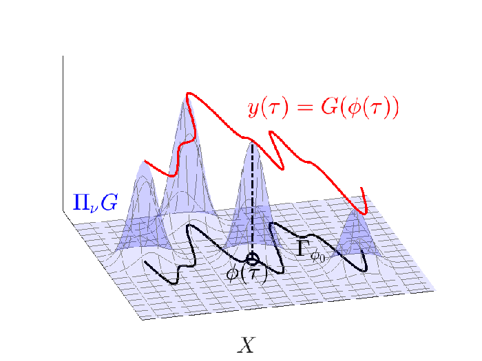
The goal is to use the continuous collection of samples to build a time-varying estimate of the unknown function .
2.1 The Offline Optimal Regression Estimate in an RKHS
We define the integral error functional to be
for the state space , some measure on , and a regularization parameter . In this equation is the evaluation functional at , which satisfies for any . The error functional can be rewritten as
The adjoint is given by for any . The study of the error functional takes a familiar structure when we introduce an operator via the identity
Note that is a time-varying operator that depends on the trajectory . In the following arguments, and later at several places in the text, the properties of the operator are important. We summarize some of its properties in the following theorem.
Theorem 1
Suppose that is a continuous admissible kernel that induces the native space of continuous real-valued functions over . The operator above is an integral operator
If there is a constant such that for all and the trajectory is continuous in time, then the operator-valued map
is continuous from to and measurable as a map from into . The operator can be understood as the Bochner integral
| (1) |
The operator is compact, self-adjoint, positive, and trace class.
Proof 1
Since is continuous and the trajectory is continuous, the map is continuous. This fact follows from the identity
and the righthand side goes to zero as by the continuity of . This identity can then be used to show that the curve is continuous as a map from from the expression
This collection of inequalities above makes repeated us of the bound . The measurability of the map from to then follows from the continuity of this map. Finally, the fact that the Bochner integral in Equation 1 exists in is a consequence of the bound
Next, we consider the compactness of . This proof essentially follows the same line of reasoning as that in Proposition 14 of [38], which is carried out for the operator and a spatial measure on . Since the operator is finite rank for each , it is trace class for each , with
The trace operator is a continuous linear operator on the trace norm class, and we know that
by the mapping property of a Bochner integral under continuous linear operators. The Bochner integral exists and is therefore trace class.
We conclude this proof by showing that is a positive operator. This is a modification of the analysis in [5], which treats a different problem where again the integral is over space, not time. For completeness, we give its outline. Let be a family of measurable subsets of with and . Fix a quadrature point from each set and define . We then have
| (2) |
where is characteristic function of the subset . The positivity of follows from the semidefiniteness of the kernel .
With these properties in hand, we can derive the optimal offline regression estimate in continuous time. In the usual way we can “complete the square” and write
Now we define the best approximation, i.e. the regressor solution in continuous time,
But it is relatively easy to calculate the Gateaux derivative of this functional in the direction . By definition it is given by
Local minima to the above minimization problem must satisfy
because the operator is invertible as a map from .
2.2 Galerkin Approximations of the Regression Estimate
The regression estimate is the solution of an operator equation in the generally infinite dimensional space . Practical algorithms must consider approximations of this solution. In this section we discuss one method for obtaining approximations based on Galerkin’s method. A review of some of the common properties of Galerkin approximations in Hilbert spaces is given in the Appendix in Section 6.1. The regression solution satisfies the equation
| (3) |
Let be some -dimensional subspace of that is used to build approximations. The Galerkin approximation is the solution of the analogous equation
| (4) |
For each we define the bilinear form to be for each . The bilinear form is bounded and coercive as defined in Section 6.1 since
By the Lax-Milgram Theorem 3 there is a unique solution of Equation 3 and of Equation 4. From Theorem 4 we know that
In the analysis so far, we have , , under the assumption that , with a native space of functions supported on the configuration space . The error in approximating the optimal regression estimate by the Galerkin estimate is bounded by the norm on the best approximation of from the subspace , but there are a number of standard techniques to build sharp bounds on the error , which depend on how regular the function is. These methods can be based on spectral analysis of integral operators and Mercer kernels, properties of the power function, or versions of the many zeros theorems [40, 19, 12]. We discuss such specific cases in the examples in Section 4.
3 Persistency of Excitation (PE) in Native Spaces
The basic error estimate for the Galerkin approximation described in Section 2.2 can be refined in several ways. In this section, we show how introducing priors on , which are certain assumptions that enforce restrictions or constraints on the unknown function, can yield improved error estimates. In analogy to the case of parametric estimation in Euclidean space, we introduce a persistency of excitation condition for flows over a manifold. The PE condition can be used to derive alternative terms of an error bound on Galerkin approximations. Define the operator
3.1 A New Persistence of Excitation Condition
In [17], we say that a persistence of excitation condition holds over the closed subspace if there exist constants such that
or in other words
| (5) |
for all and . Note that the above PE condition uses the operator as given in Equation 1. We analyze two different cases below:
- (1)
The space is the native space generated by a subset ,
Note that in this case equipped with the norm it inherits as a closed subspace of .
- (2)
The space is selected to be the closed subspace that is defined in terms of a fixed, compact, self-adjoint, positive operator and its spectral decomposition.
3.2 Persistency in with
Note that, if the above PE condition in Equation 5 holds, we obtain upper and lower bounds on . For simplicity, suppose that for some integer . Then, if the PE condition holds for , we know that
for all . This means that for all we have the upper bound
3.2.1 The Optimal Regressor in
We can use the above bound to find an error bound for the best offline estimate . Suppose that is the -orthogonal projection onto the closed subspace . We set
We define the error between the offline estimate and to be . It follows that
Now we apply the bound on , and we get
But, by virtue of , we know that . Assuming that is Lebesgue measure on and , we obtain
| (6) |
In particular, if we have , we conclude that
3.2.2 The Optimal Regressor in
Above we characterized the optimal regressor when the subspace is PE. It is also possible to pose the original regression problem in and seek the optimal regressor when is PE. In this case we seek the approximation that satisfies the equation
Then the solution can also be written as
We can apply the PE condition
for all . This gives an upper bound
for all . In this case, , so that the error can then be expressed as follows
We can bound each of the two terms on the right hand side of the equality by writing
We now have the error bound
| (7) |
Observations:
- 1.
- 2.
Note that the bound on given by Equation 6 consists of three terms that each behave differently as . The first term converges to a constant proportional to the projection error as . The second term decays to zero as . However, the last term, referred to as the drift term, grows indefinitely as . If we seek to compute the optimal estimate via continuous regression when only is PE, this drift term results. The primary issue is that we cannot apply the PE condition
on because . This problem is addressed by seeking the optimal regressor that filters out this drift term. This error is bounded by only two terms as given in Equation 7 where the first converges to a constant proportional to and the second decays to zero as .
- 3.
In a typical situation, in applications to finite dimensional approximations, it is frequently the case that consists of a finite number of samples, , and then
In this case, the error between the best offline estimate and the projection can be bounded above by the rate of convergence of to zero. This is carried out in detail in the example in Section 4.
- 4.
Since the operator is compact, if the PE condition in Equation 5 holds for , it must be the case that is finite dimensional. Otherwise, the PE condition would imply that the compact operator has a bounded inverse, which is impossible on an infinite dimensional space . It follows that the primary application of case (1) will be to understand convergence of the optimal regressor when finite dimensional subspaces of approximants are PE.
3.2.3 Approximation: Method (1)
The exact optimal solution of the regression problem in continuous time, given by , or correspondingly defines a function of time and space, for and . Practical implementations and algorithms must employ approximations of the exact regression solution. As in methods for parametric estimation in Euclidean spaces, recursive methods to approximate the solution of this problem are often used. We have studied one recursive method for the problem in this paper in [14]. Here, and in the numerical examples in Section 4, we comment on implementations of offline approximations. Let be the approximation of either or . When we define the approximation using the continuous regression error functional, we obtain an equation that has the form
| (8) |
Note also that the optimal estimate in the continuous case requires integrating the kernel functions along the orbit, which ordinarily cannot be directly calculated in closed form. Consequently, the approximation requires approximating the integral term. For a function , a general form of a quadrature rule builds the approximation
where is the number of quadrature points, are the quadrature weights, and are the quadrature points. The approximation of the integral can be determined from a multitude of different quadrature techniques. Standard examples include the trapezoidal rule, Simpsons rule, or Gaussian quadratures. Here we use a particularly simple quadrature rule. Recall the above definitions of , the subintervals , and the quadrature points for from the proof of Theorem 1 where the weights are given by the time intervals . One form of approximating the integral via a one point quadrature rule generates the equation
| (9) |
We end this section with the pseudo-code implementation in Algorithm 1 to explicitly determine the estimate from this approximation method. Note that the initialization steps require that we select samples that have sufficient distance between one another ensuring the calculation of stable numerical estimates. [31, 40]
3.2.4 Approximation: Method (2)
The system of Equations 9 above requires the introduction of quadratures over . In this section, we introduce a second method of approximation that eliminates the calculation of quadratures. The coefficients of the second method of approximation satisfy the following equation
| (10) |
In the above equation the unknown coefficients are now inside the integrand and are integrated along the orbit. Taking the time derivative of Equation 10 we can get an evolution equation for the coefficients . It is given by
| (11) | ||||
As opposed to the previous approximation method, estimates constructed according to Equation 11 evolve continuously according to the ODE given by Equation 11, rather than approximations generated by Equation 8. As opposed to the previous offline optimization problem, this approximation method could, in principle, generate and update estimates in real-time. We emphasize that the theory presented in this paper only applies to Method (1), and we leave the theoretical study of Method (2) for a future paper. However, for completeness, we examine the performance and convergence behavior of both methods in the numerical results of this study.
Like the Method (1), we present Algorithm 2 to outline the steps needed to implement this approximation method.
3.3 Learning Theory and the Regression Estimate
In this section, we give an expanded discussion of the similarities and differences between the approximations described in Sections 3.2.3 and 3.2.4 in this paper and related techniques in distribution-free learning theory, statistical learning theory, and machine learning theory. For the most part, these learning theory approaches focus on estimates generated from samples of discrete, independent and identically distributed (IID) stochastic systems. See [18, 41] for popular summaries of the state-of-the-art in these fields. Learning theory in general [37] is concerned with a number of distinct problems including pattern recognition, classification, and function estimation. The learning problem for function estimation involves approximating a mapping from a set of inputs to elements in an output space . It is commonly assumed that the data is a collection of noisy sample pairs that are generated from a discrete IID stochastic process defined by the probability measure on . Ideally, optimal estimates of are defined to be minimizers of the functional , commonly referred to as the expected risk,
where is a joint measure on the sample space . Note that the measure can be rewritten, , where is the conditional measure on given and is the marginal measure on the input space . In principle, the ideal minimizer of is given by
with referred to as the regressor function. However, the measures , , and are generally unknown, and the ideal solution, above cannot be computed in practice. It is this reason that the above problem is said to define a type of distribution-free learning problem [18].
Since the regressor cannot be computed in general, standard approaches in machine learning theory replace the error functional above with its regularized, discrete counterpart
that is defined in terms of the samples of a discrete IID stochastic process. Here is the regularization parameter and is a space of functions that has a norm that measures smoothness. When some finite dimensional space is used to construct approximations, the method of empirical risk minimization (ERM) seeks the function that is the minimizer
Note that the minimizer depends on the number of samples and the number of basis functions . The convergence of as and increase is a well-studied topic, certainly one of the most well-known in learning theory. Again, see [18, 41] for a complete description of the myriad of approaches to this problem. The relationship of the approach in this paper to the standard learning problem can be made more precise by assuming that the basis is taken to be that is the scattered basis as we use in Equations 10 and 11. In this case, it is well-known that where the coefficients satisfy
| (12) |
These equations should be carefully compared to Equations 8 and 10. In Equation 12 the inner summation is over the samples from an IID process see [6, 36]. For the regression problem in continuous time in Equation 8, the inner summation above is replaced with an integration in time along a trajectory. We see that the use of one point quadrature rule in time, which yields Equation 1, generates a set of algebraic equations that have a similar structure to that which arises in learning theory for discrete stochastic processes in Equation 12. In fact, if the sample times are uniformly distributed, the weights of integration are constant and can be cancelled in Equation 8. In such a case, the two sets of equations have identical form. Although the form of the equations is the same, the error analysis for the two cases differs substantially. One significant difference is that, in the typical learning theory scenarios, it is assumed that samples are dense in , while this is a rather special case for deterministic dynamical systems. For dynamical systems, the set over which the error analysis is performed is typically unknown. The set of samples along a trajectory can be dense in a very irregular set. This fact is emphasized in the numerical example in Section 4. Additionally, the error analysis for Equation 8 relies on a PE condition that is not part of the stochastic framework. The error analysis of Equation 12 usually results from taking the expectation. For deterministic dynamical systems, however, there is no definition of expectation. This work instead considers when the inputs are generated along a trajectory governed by some underlying, generally unknown evolution. For a more in-depth discussion of learning theory for unknown discrete samples, see the work of Cucker and Zhou in [5] or Devito et. al. in [33].
3.4 Subspaces Chosen as a Spectral Space
The case studied above suffices to derive rates of convergence of approximations in finite dimensional spaces where is a finite set of points. From a practical point of view, the results apply to many important cases that can be implemented. However, from a theoretical point of view, we would like to be able to identify a closed subspace that is “as large as possible” in the definition in Equation 5. It is of interest therefore to find a space that is infinite dimensional and satisfies the PE condition. We do this by introducing spectral approximation spaces associated with a fixed, compact, self-adjoint operator . By the spectral theorem for compact, self-adjoint operators, this means that the operator can be expressed as
where is the sequence of eigenvalues arranged in nonincreasing order and repeated as needed for multiplicity, and is a corresponding -orthonormal collection of eigenfunctions. The only possible accumulation point of the eigenvalues is zero. In the following we always assume that as , since if the sum above terminates after a finite number of terms, all the approximation spaces introduced below degenerate and are equivalent. We also assume that the kernel of is equal to . By [33] Proposition 8, the eigenvectors of span , so in the case at hand are an orthonormal basis for .
By virtue of the functional calculus for compact, self-adjoint operators, the operator is well-defined for all by the expansion
We define the spectral approximation space to be
where the norm is given by
The spaces have a long history and are closely related to approximation spaces. [30, 7]. Since , the weight grows as . The space consists of functions in whose generalized Fourier coefficients converge faster than increases. It can be shown that these spaces are nested with whenever . It should also be noted that . So, in particular we have . In the language of approximation theory, the define a scale of spaces for containing functions of increased (generalized) smoothness as increases.
The following theorem provides the technical connection between the spaces and spectral space in terms of the operator .
Theorem 2
We have the equivalence
for all and is an isometry.
Proof 2
Suppose . Then
It is also immediate that , so is an isometry from onto . In particular is an isometry.
In view of Theorem 2, when the PE condition holds, we have constants such that
for all and . Note that this equivalence holds uniformly for the family for all . This pair of inequalities can also be interpreted as the statement that on
Now we return to the study of the error when we choose , and we seek the optimal . In analogy to Case 1, we set
| (13) | ||||
| (14) |
Following the same plan of attack as in Case 1, we obtain
In this case, in contrast, we can write
for all . In other words restricted to is a bounded linear operator that satisfies
| (15) |
By definition, and . Since , we can apply the bound in Equation 15 to Equation 14. The remainder of the proof is unchanged and we conclude that, if ,
Observations:
- 1.
It should be emphasized that the operator is compact, as described in Theorem 1. But when the PE condition holds with , it is not compact as an operator . It is boundedly invertible as a map from .
- 2.
Intuitively, the PE condition can be understood as a statement that the local approximation space defined over the small time-span in terms of the operator is spectrally equivalent to the global approximation space defined over in terms of .
4 Numerical Examples
The error estimates above apply to quite general situations. Since some of our earlier works in [27, 23, 31] have included numerical examples with evolutions on compact manifolds, here we model a trajectory that is dense in a complicated, unknown subset in . Consider the Lorenz system
for . Figures 2(a) and 2(b) illustrate orbits of the system for various initial conditions. Set and denote by . The complex nature of the trajectories of this system has been studied and commented on so extensively that it is now understood as an exemplar of what chaos and complexity is, even in the popular press.


There are a number of Lyapunov functions that have been introduced to study the long-term behavior of this system. One common choice is
for all . Its derivative along trajectories is given by
which is negative outside of the compact set
The fact that this set is compact follows by demonstrating that the boundary of the set is an ellipse given by
Given that is continuous and that points inside the ellipse satisfy the following inequality
it is clear that the set is the closure of the interior of the ellipse. Since is compact and is continuous, the maximum of over is achieved, . Define the dilation of the set by some parameter to be
The set is positive invariant. Any trajectory starting at is guaranteed to enter in finite time and never leave this set. This means that for any initial condition , the orbit is precompact, that is, is compact. From standard results on dynamical systems [39], it is known that the positive limit set of a precompact trajectory , which is defined by
is compact. In fact, we have
Both and are guaranteed to be compact sets, but they can be highly irregular. For the case at hand, where we study the Lorenz system, this fact is well-known.
We want to use the results of this paper to understand what can be said about the regression problem in continuous time for this system, and we are particularly interested in what the error bounds imply for estimates of an observable function for this system. We would like to understand how the trajectory affects convergence of approximations, and to determine in what spaces the continuous time regression problem converges. We can use either of the sets or to study the convergence properties.
In this paper, we study the case when the set . We define different sets that have samples in , . We assume that these are nested, . Associated with we define the space of approximants in terms of a scattered basis with . These finite dimensional spaces of approximants are data driven: they are generated along a trajectory of the system. For each , suppose that the PE condition holds for . Whether or not the PE condition holds in the case that can be verified by conditions related to the visitation, or time of occupation, of the trajectory in neighborhoods of the samples in . See [17, 26, 27] for a discussion. If the trajectory persistently excites the subspace , we have the estimate from Equation 7
Concrete estimates of the rate of convergence of this expression can be obtained using the power function over the set
| (16) |
where is the kernel that defines the native space . It is well-known [40, 42] that the power function enables the pointwise bound
This pointwise bound can be used to derive a corresponding bound on , for smooth enough . The details exceed the length of this brief paper and are given in [3] in a different application to approximation of Koopman operators, or this bound can be inferred from the proof of Theorem 11.23 in [40]. Ultimately, we obtain a bound
for all that are smooth enough, which means that the optimal regression estimate in continuous time satisfies
| (17) | ||||
| (18) |
for all smooth enough.
We begin with an assessment of the numerical implementation of Method (1). We illustrate the performance of an estimate defined in Equation 8 of generated over an orbit of the Lorenz system. We only pose the regression problem over a projection of the orbit onto the plane so that the results are easy to visualize. The function we estimate is given by
and we choose the initial condition . In this example, we use the Matern-Sobolev kernel,
with the standard Euclidean norm over , , and the hyperparameter . In Figure 3, the output for is represented by the red curve that hovers over the dynamics of the input orbit labeled by the black curve in the plane. In this figure, 126 kernel centers are selected quasi-uniformly along the orbit with a separation distance of around 2 and the regularization parameter .

From the figure, it is clear that the approximation represented by the colored mesh yields, qualitatively speaking, a good estimate of the true function (the green surface) over the orbit.
When interpreting this result, it is important to keep several facts in mind.
Observations:
- 1.
The theory in this paper uses the compact subset , whose regularity is not easy to characterize. The set defines the space in which regression approximations in continuous time converge.
- 2.
The convergence of estimates is in the space , which is an RKHS space of funnctions over the set . Even though is quite irregular, the functions in are supported on the whole set , not just . This means that estimate is, in a sense, “naturally extended” to the whole state space . In the case at hand, the set has zero Lebesgue measure. Even though the trajectory or orbit may not reach some points or subsets of , the function estimates are well-defined everywhere nonetheless.
4.1 Example: Characteristics of Approximation Method (1)
The next set of results examines the estimates of approximation Method (1) over orbits spanning different intervals of time. Using the same underlying input dynamics, kernel function, hyperparameter , regularization parameter , and unknown function from the previous results, each of the estimates are generated from an orbit starting at an initial condition . The centers are placed quasi-uniformly along the orbit with a separation distance of around 2. Figures 4(a) through 4(d) illustrate the estimates calculated over different spans of time. In Figure 4(a), we can see that, even for small time intervals, the error between the estimate and the true function begins to diminish significantly over the orbit. Additionally, there is significant decrease in the error over the trajectory as seen in Figures 4(a) and 4(b). While the error continues to decrease as , it is evident the error reduction between Figures 4(c) and 4(d) occurs at a much smaller rate than the previous time intervals. This is a consequence of diminishing rate of reduction in the power function as and more samples are collected.


For the next set of figures, we examine the effects of the regularization penalty term of used in approximation Method (1) by varying the choices of . In order to examine the influence of the regularization parameter on the long-term convergence behavior, each simulation is run over a sufficiently long time interval of 200 seconds. Using the same Lorenz system, kernel function, hyperparameter , unknown function , initial conditions, and center spacing as the previous results, Figures 5(a) through 5(d) illustrate the estimates for different values of . Overall, these four graphs depict qualitative behavior that is well-known in the field of inverse problems. The error functional introduced in Section 2.1 balances two terms
Minimizing term 1 decreases the error over the orbit , while term 2 penalizes the size of the estimate as measured in the norm. Increasing generally leads to smoother estimates. Additionally, it also reduces the chance of over-fitting, which can lead to poor estimates in the presence of a noisy or perturbed data set. This classic phenomenon is studied in great depth in texts like [8]. With these considerations in mind, proper estimates can be generated by selecting a particular choice of to effectively regularize the estimate.


4.2 Example: Characteristics of Approximation Method (2)
The next set of results examine how the estimates generated using approximation Method (2) vary in time and converge as . Using the same conditions as the previous results, the estimate was initialized with all coefficients for and the states initial condition . Figures 6(a) through 6(d) illustrate the estimate generated after different amounts of time. In contrast to the previous approximation method, these figures depict the evolution of a single estimate as . As mentioned previously, this approximation is determined by an evolution of coefficients . The evolution law minimize the integrated error for over the orbit for time rather than computed an offline optimal solution at a specific time. At early stages of the evolution such as Figure 6(a), samples predominantly aggregate near one of the unstable equilibrium points. However, as the trajectory approaches the second equilibrium, it begins to influence the coefficients of the nearby centers and decrease the error between the estimate and . Figures 6(c) and 6(d) suggest that the estimate converges to the projection over the domain of attraction as more time passes and more samples are collected. Similar to the estimate from approximation Method (1), there is an initial rapid change in the error over the trajectory. While the error appears to decrease for longer periods of time, it is evident that the error reduction between Figures 6(c) and 6(d) occurs at a much lower rate than the reduction seen from Figure 6(a) to 6(b) and Figure 6(b) to 6(c).


Using the same conditions as those used in the regularization study of approximation Method (1), we also examine the effects of the regularization term on the estimate from approximation Method (2) by building estimates using different choices of . Figures 7(a) through 7(d) illustrate the estimates for different values of . In these estimates, the term also plays a role in the transient response of the coefficients’ evolution. From the figures, it is evident that a larger decreases the sensitivity to changes in the estimate as new samples are collected over time. Consequently, the numerical study suggests better convergence of the estimates may require a larger number of samples when is large. By decreasing , the estimates are more responsive to changes in the data as seen in Figure 7(c). However, even without noise or disturbances, smaller values of can yield large oscillatory behavior in the estimate as seen in Figure 7(d). This example indicates that must be carefully selected for a desired transient response in the second approximation method.


4.3 Example: Human Kinematics Study
This example uses three-dimensional motion capture data from a subject running along a treadmill [11]. From the experiment, 17,000 marker coordinates are collected relative to a fixed inertial frame defined by the camera’s position. For this example, a small candidate kinematic model is defined in terms of the full collection of experimental trajectories. The marker coordinates of the hip, knee, and ankle in the full data set are projected onto the sagittal plane that divides the left and right half of the body, see Figure 8.
With this projection, the first input is defined to be the joint angle . It is measured between the projected vector that connects the hip to knee and the body-fixed vector in the plane, and it roughly corresponds to hip flexion. The second input comes from the knee flexion angle . It is measured between the vector and , the vector connecting the knee to the ankle projected to the sagittal plane. These choices of projections and associated degrees of freedom are taken to define a low-dimensional but unknown dynamic system. We seek to estimate outputs of the unknown dynamic system.
For illustrative purposes, we chose to estimate the projection of the kinematic map from the joint angles and to the ankle coordinate associated with the body-fixed vector. Figure 9(a) and 9(b) show the approximations of over an orbit in the input space defined by the coordinates and . The estimates are generated for both approximation Method (1) and (2), respectively. In both estimates, the Matern-Sobolev kernel with is used. Additionally, the kernel centers for both estimates are chosen so that there is sufficient separation distance of at least 10 radians between each of the kernel centers, . As mentioned previously, the two estimates respond differently to the regularization term. A relatively small regularization parameter was selected for the estimate from approximation Method (1). The second approximation exhibited oscillations over the data for small values of . Consequently, we increased the regularization parameter to for the estimate from the second approximation method.
When comparing these approximations there are a couple of key things to note. The estimate using the second approximation method in this study is generated using a continuous evolution law as given by Equation 11. However, the collected data consists of discrete sets of motion capture data collected at discrete times. In order to utilize the collected data and also have a continuous evolution update, we use MATLAB’s built-in functions to fit splines that are continuous in time with knots at the discrete states. This builds a continuous approximation of the orbit over small time intervals. While the approximation given by Method (1) does not need this step, we must approximate the integral over the orbits given the discrete data and a particular quadrature rule. Consequently, the estimate of Method (1) is susceptible to error associated with quadrature approximations.


5 Conclusions
In this paper, an optimal, offline estimation problem is formulated for continuous time regression over state spaces that include certain types of smooth manifolds. A new persistency of excitation condition is introduced that is well-defined for flows on manifolds, and it is used to obtain sufficient conditions for convergence. Error estimates are derived that characterize the rate of convergence of finite dimensional estimates of the solution of the regression problem in continuous time over manifolds. We then discuss two methods to generate finite-dimensional approximations of the optimal regression estimate. Numerical simulations are presented to better illustrate the qualitative behavior of the two approximation methods. Finally, we discuss and analyze results on estimating functions over motion capture data to demonstrate how to implement the algorithm on experimental data.
6 Appendix
6.1 Background on Galerkin Approximations
Let be a real Hilbert space, be a bounded linear operator on , be a fixed element of , and suppose we seek to find that satisfies the operator equation
It is customary that the existence and uniqueness of the solution of this equation is established by studying the associated bilinear form given by for all . Then the operator equation above is equivalent to finding the for which
| (19) |
The Lax-Milgram Theorem given below stipulates a concise pair of conditions that ensure the well-posedness of the operator equation.
Theorem 3 (Lax-Milgram Theorem [4])
The bilinear form is bounded if there is a constant such that
and it is coercive if there is a constant such that
If the bilinear form is bounded and coercive, then and there is a unique solution to Equation 19.
Proof 3
The first condition above, continuity of the bilinear form, ensures that by definition. The coercivity condition implies that the nullspace of is just . As a result, we know that is one-to-one. This means that the operator is well-defined. From the coercivity condition we also conclude that
for every . This means that and .
One implication of the fact that is that is closed. Suppose that and . By construction there is a sequence such that . But we have
and is a Cauchy sequence in the complete space . There is a limit . By the continuity of the operator , we know that , hence . The range of is consequently closed.
It only remains to show that . Suppose to the contrary there is a with . Since , we know that
By the coercivity condition, we must have . But this is a contradiction and is all of .
Next, we discuss how error bounds are derived for Galerkin approximations of the solution of the operator equations above. Let be a finite dimensional subspace of . By definition, the Galerkin approximation is the unique solution of the equation
| (20) |
The theorem below summarizes one of the well-known bounds on the error between the Galerkin approximation and the true solution .
Theorem 4 (Cea’s Lemma, [4])
Proof 4
First, note that when satisfies the boundedness and coercivity conditions, its restriction to satisfies the boundedness and coercivity conditions with the same constants relative to . This means that the Galerkin equations have a unique solution . Since Equation 19 holds for all , it holds for all . We can subtract Equations 19 and 20 for each and obtain
for each . Using the boundedness and coercivity of the bilinear form, as well as the orthogonality of the error, we have
for any . The theorem now follows after canceling the common term on the right and left.
References
- [1] Bai, S., Wang, J., Chen, F., Englot, B.: Information-theoretic exploration with bayesian optimization. In: 2016 IEEE/RSJ International Conference on Intelligent Robots and Systems (IROS), pp. 1816–1822. IEEE (2016)
- [2] Berlinet, A., Thomas-Agnan, C.: Reproducing kernel Hilbert spaces in probability and statistics. Springer Science & Business Media (2011)
- [3] Burns, J., Estes, B., Guo, J., Kurdila, A.J., Liu, R., Paruchuri, S.T., Powell, N.: Approximation of koopman operators: Domain exploration. submitted to the 2022 CDC (2022)
- [4] Ciarlet, P.G.: Linear and nonlinear functional analysis with applications, vol. 130. Siam (2013)
- [5] Cucker, F., Zhou, D.X.: Learning Theory: An Approximation Theory Viewpoint. Cambridge Press (2007)
- [6] DeVore, R., Kerkyacharian, G., Picard, D., Temlyakov, V.: Mathematical methods for supervised learning. IMI Preprints 22, 1–51 (2004)
- [7] DeVore, R.A., Lorentz, G.G.: Constructive approximation, vol. 303. Springer (1993)
- [8] Engl, H.W., Hanke, M., Neubauer, A.: Regularization of inverse problems, vol. 375. Springer Science & Business Media (1996)
- [9] Farrell, J.A., Polycarpou, M.M.: Adaptive approximation based control: unifying neural, fuzzy and traditional adaptive approximation approaches, vol. 48. John Wiley & Sons (2006)
- [10] Foster, D., Sarkar, T., Rakhlin, A.: Learning nonlinear dynamical systems from a single trajectory. Learning for Dynamics and Control, PMLR (2020)
- [11] Fukuchi, C.A., Fukuchi, R.K., Duarte, M.: A public dataset of overground and treadmill walking kinematics and kinetics in healthy individuals. PeerJ 6, e4640 (2018)
- [12] Fuselier, E., Wright, G.B.: Scattered data interpolation on embedded submanifolds with restricted positive definite kernels: Sobolev error estimates. SIAM Journal on Numerical Analysis 50(3), 1753–1776 (2012)
- [13] Gao, T., Kovalsky, S.Z., Daubechies, I.: Gaussian process landmarking on manifolds. SIAM Journal on Mathematics of Data Science 1(1), 208–236 (2019)
- [14] Guo, J., Kepler, M.E., Paruchuri, S.T., Wang, H., Kurdila, A.J., Stilwell, D.J.: Strictly decentralized adaptive estimation of external fields using reproducing kernels. arXiv preprint arXiv:2103.12721 (2021)
- [15] Guo, J., Paruchuri, S.T., Kurdila, A.J.: Approximations of the reproducing kernel hilbert space (rkhs) embedding method over manifolds. In: 2020 59th IEEE Conference on Decision and Control (CDC), pp. 1596–1601. IEEE (2020)
- [16] Guo, J., Paruchuri, S.T., Kurdila, A.J.: Approximations of the reproducing kernel hilbert space (rkhs) embedding method over manifolds. In: 2020 59th IEEE Conference on Decision and Control (CDC), pp. 1596–1601. IEEE (2020)
- [17] Guo, J., Paruchuri, S.T., Kurdila, A.J.: Persistence of excitation in uniformly embedded reproducing kernel hilbert (rkh) spaces. In: 2020 American Control Conference (ACC), pp. 4539–4544. IEEE (2020)
- [18] Gyorfi, L., Kohler, M., Krzyzak, A., Walk, H.: A Distribution-Free Theory of Nonparametric Regression. Springer (2002)
- [19] Hangelbroek, T., Narcowich, F.J., Ward, J.D.: Polyharmonic and related kernels on manifolds: interpolation and approximation. Foundations of Computational Mathematics 12(5), 625–670 (2012)
- [20] Hovakimyan, N., Cao, C.: Adaptive Control Theory: Guaranteed Robustness with Fast Adaptation. SIAM (2010)
- [21] Ioannou, P.A., Sun, J.: Robust adaptive control. Courier Corporation (2012)
- [22] Krstic, M., Kanellakopoulos, I., Kokotovic, P.: Nonlinear and Adaptive Control Design. John Wiley & Sons (1995)
- [23] Kurdila, A.J., Guo, J., Paruchuri, S.T., Bobade, P.: Persistence of excitation in reproducing kernel hilbert spaces, positive limit sets, and smooth manifolds. arXiv preprint arXiv:1909.12274 (2019)
- [24] Liu, G.H., Theodorou, E.A.: Deep learning theory review: An optimal control and dynamical systems perspective. arXiv preprint arXiv:1908.10920 (2019)
- [25] Narendra, K.S., Annaswamy, A.M.: Stable Adaptive Systems. Dover (1989)
- [26] Paruchuri, S.T., Guo, J., Kurdila, A.: Kernel center adaptation in the reproducing kernel hilbert space embedding method. arXiv preprint arXiv:2009.02867 (2020)
- [27] Paruchuri, S.T., Guo, J., Kurdila, A.: Sufficient conditions for parameter convergence over embedded manifolds using kernel techniques. arXiv preprint arXiv:2009.02866 (2020)
- [28] Paruchuri, S.T., Guo, J., Kurdila, A.: Kernel center adaptation in the reproducing kernel hilbert space embedding method. International Journal of Adaptive Control and Signal Processing (2022)
- [29] Paruchuri, S.T., Guo, J., Kurdila, A.J.: Sufficient conditions for parameter convergence over embedded manifolds using kernel techniques. IEEE Transactions on Automatic Control (2022)
- [30] Pietsch, A.: Approximation spaces. Journal of Approximation Theory 32(2), 115–134 (1981)
- [31] Powell, N., Liu, B., Kurdila, A.J.: Koopman methods for estimation of animal motions over unknown, regularly embedded submanifolds. arXiv preprint arXiv:2203.05646 (2022)
- [32] Qianxiao, L., Weinan, E.: Machine learning and dynamical systems. SIAM News pp. 5–7 (2021)
- [33] Rosasco, L., Belkin, M., Vito, E.D.: On learning with integral operators. Journal of Machine Learning Research 11, 905–934 (2010)
- [34] Sastry, S., Bodson, M.: Adaptive control: stability, convergence and robustness. Courier Corporation (2011)
- [35] Smola, B.S.A.J.: Learning with Kernels: Support Vector Machines, Regularization, Optimization, and Beyond. MIT Press (2002)
- [36] Temlyakov, V.: Multivariate approximation, vol. 32. Cambridge University Press (2018)
- [37] Vapnik, V.N.: An overview of statistical learning theory. IEEE transactions on neural networks 10(5), 988–999 (1999)
- [38] Vito, E.D., Rosasco, L., Toigo, A.: Learning sets with separating kernels. Applied and Computational Harmonic Analysis pp. 185–217 (2014)
- [39] Walker, J.: Dynamical Systems and Evolution Equations: Theory and Applications. Springer (2013)
- [40] Wendland, H.: Scattered data approximation, vol. 17. Cambridge university press (2004)
- [41] Williams, C.K., Rasmussen, C.: Gaussian processes for machine learning. MIT Press (2006)
- [42] Wittwar, D.W., Santin, G., Haasdonk, B.: Interpolation with uncoupled separable matrix-valued kernels. arXiv preprint arXiv:1807.09111 (2018)
Statements and Declarations
The authors declare that no funds, grants, or other support were received during the preparation of this manuscript. The authors have no relevant financial or non-financial interests to disclose. The datasets generated during and/or analysed during the current study are available from the corresponding author on reasonable request