Full time-dependent counting statistics of highly entangled biphoton states
Abstract
Highly entangled biphoton states, generated by spontaneous parametric processes, find wide applications in many experimental realizations. There is an increasing demand for accurate prediction of their time-dependent detection. Unlike approaches that have emerged so far, this paper presents an approach providing full time-dependent counting statistics in terms of efficiently computable formulas, valid for a wide range of entanglement and arbitrary interaction times. General spatial modes are taken into account to describe free space and fiber propagation. The time intervals that correspond to the statistics are classified according to their widths. Apart from large and small widths compared to the temporal correlation width, intermediate interval widths give access to accidental correlations between separated time intervals. Moreover, the approach is easily applicable to a modular array of arbitrary optical components and external influences. This is demonstrated on phase-time coding, where the detuning of the interferometers affecting Franson interference is investigated. An acceptable range for the detuning is estimated, such that the security of the key is not compromised.
I Introduction
Quantum entanglement is one of the most useful resources in quantum information technologies and is fundamental for secure information processing and communications. In particular, a high degree of entanglement is attractive for its high data capacity and error resilience Xie_2015. Bipartite states with continuous variables (CV) enable a degree of entanglement, which might be much higher than the maximal achievable degree of entanglement with respect to (w.r.t.) discrete variables Mikhailova_2008. One of the most conventional methods in CV is presently the generation of entangled photons by spontaneous parametric processes, such as spontaneous parametric down-conversion (SPDC) and spontaneous four-wave mixing (SFWM). These processes generate photon pairs with a strong spectral and temporal correlation, where each photon is transmitted to a party (conventionally referred to as Alice and Bob). It plays a major role in quantum cryptography (QC) since the detection of one photon heralds the presence of the other. Highly entangled biphoton states find a wide application in many experimental realizations. Frequency-bin entanglement Imany_2018, frequency multiplexing Joshi_2018, nonlocal dispersion cancellation (NDC) Li_2019, and quantum electro-optic circuits Luo_2020 were recently investigated using a continuous-wave pump laser. Although perfect frequency entanglement can thus be achieved Zhai_2017, it is inadequate for many applications requiring timing information since the emission time of the photon pairs is completely random Quan_2015. Hence, pulsed pumps with well-defined emission times were recently realized to generate highly entangled photon pairs, where entanglement properties Quan_2015 and NDC Xiang_2020; Lerch_2017; Hu_2015 have been investigated. Pulsed pumps have also found great applications in areas such as arrayed waveguide grating Matsuda_2017, on-chip generation Kues_2017, time-bin implementation Martin_2017, and quantum key distribution systems Lee_2014; Arahira_2016.
A specific application of pulsed pumps is phase-time coding, which was first proposed by Brendel et al. Brendel_1998 and has been experimentally realized Stucki_2006. This is a promising approach for QC since coding in time basis is particularly stable and the coherence length of the pump laser is not critical Gisin_2001. The setup includes a Franson arrangement, which comprises two unbalanced Mach-Zehnder interferometers (MZIs) and is widely used in several applications, such as gate operations Lo_2020, superdense coding Pavicic_2016, and chip-based microresonators Peacock_2016. The key bits are first established based on the photon pair’s temporal correlation. Hence, there is a strong demand for an accurate prediction of this correlation with ever-increasing precision Mueller_2020. A second basis to establish the key bits is implemented using Franson interference, which can be achieved by adjusting the phases of the MZIs. To ensure perfect correlation, the optical path lengths of the MZIs must differ less than the coherence length of the entangled photons Gao_2019. Otherwise, Franson interference is affected, culminating in its complete disappearance if the detuning of the MZIs exceeds the coherence length. Since the security of the key relies on perfect correlation, full knowledge of this influence is indispensable. In particular, an acceptable range of the detuning without compromising the security of the key is of substantial interest for experimental realizations of phase-time coding. For a detailed description, however, many kinds of temporal information must be taken into account, such as the width of the pulsed pump, required for coding in time basis, and the detailed temporal correlation, which determines Franson interference in the case of small detuning. At the same time, a precise description of detecting multiple photon pairs should be provided since uncorrelated photons cause accidental coincidences, which must be discarded during key distillation Takesue_2010; Gisin_2001. Due to wide applications and decisive advantages of high entanglement, an arbitrarily high degree of entanglement should also be allowed, in particular the limit of perfect entanglement.
A detailed description of Franson interference for small detuning, however, has only been poorly addressed yet. Although many different approaches have emerged so far, none of them is suitable for this task since they do not fulfill all aforementioned requirements at the same time. For instance, modeling each pulse as orthogonal states Yan_2021; Lo_2020; Ikuta_2016; Martin_2017; Takeoka_2015; Richart_2012 neglects many kinds of temporal information. Another way in which they are taken into account is the perturbative limit of low mean photon number Zhai_2017; Hou_2016; Quan_2015; Xie_2015; Phehlukwayo_2020; Xiang_2020; Liu_2020; Dorfman_2021. Although this approach was recently used to investigate Franson interference for increasing detuning of the MZIs Lukens_2013; Zhang_2021, the generation of multiple photon pairs is neglected. This, however, is of particular importance for phase-time coding due to serious consequences on the security of the key Gisin_2001.
Another approach is to assume perfect entanglement Kuklewicz_2005 or to approximate the strong temporal and spectral correlation, respectively, by a diagonal matrix of discrete bins Wang_2020; Kues_2017. This approach has been applied to investigate spatial quantum correlations Brambilla_2004 and to derive full counting statistics Signorini_2020; Takesue_2010. The detailed temporal correlation between entangled photons, however, is neglected. This is incompatible with modeling of Franson interference for small detuning of the MZIs. Further approaches, such as Schmidt decomposition Mauerer_2009 and general optical modes Burenkov_2017, provide full knowledge of the quantum state Lamata_2005; Law_2004. Although the latter approaches include all physical information, even pump field depletion Perina_2016, the computational effort increases significantly for higher entanglement since more modes contribute, hence an exceedingly time and resource consuming approach. Many experimental realizations can thus not be modeled suitably since improving the degree of entanglement is of broad interest. In particular, the limit of perfect entanglement remains an open problem.
In this paper, a theoretical approach is presented providing full time-dependent counting statistics of photon pairs generated by spontaneous parametric processes in terms of efficiently computable formulas. The joint amplitude may be chosen arbitrarily. General spatial modes and two widely adopted communication channels, free space and fiber propagation Xu_2020, are discussed. For the latter channel, the corresponding time intervals are classified into two types: Their widths are much smaller and their widths are much larger than the temporal correlation width. The first case provides the computation of general correlation functions, whereas the second case is important for coding in time basis. Intermediate interval widths are investigated by expanding the latter liming cases, giving access to a more precise prediction of accidental correlations between separated time intervals. The approach is valid for a high degree of entanglement and likewise for a low degree if the mean photon number is bounded by . The higher the entanglement, the larger . In the case of low entanglement, the mean photon number is restricted by , which corresponds to the perturbative limit. In the case of high entanglement, the limitation can be neglected due to . The first steps of this approach were derived in a previous work Master-Thesis and the present paper shows it completely.
In the case of further optical components and external influences, the approach can be generalized by simple modifications of the derived formulas. To this end, a general procedure is presented, which can be easily applied to a modular array of arbitrary components and influences. This is applied to the setup of phase-time coding. To demonstrate the usefulness of this approach, full counting statistics of Franson interference are derived and detection probabilities are presented for increasing detuning of the MZIs. By means of these results, an acceptable range for the detuning is estimated, such that the security for practical QKD installations is not compromised. This could not be achieved before since, unlike previous approaches, the requirements to accurately describe Franson interference for increasing detuning are fulfilled. All temporal information and multiple photon pairs effects are taken into account. Since the derived formulas are efficiently computable, they can be easily applied to an arbitrarily high degree of entanglement.
The paper is organized as follows: After the description of biphoton states generated by spontaneous parametric processes in Sec. II, the general photoelectric counting statistics are presented in Sec. III. Even though there is no systematic numerical treatment of the general statistics, Sec. IV provides the statistics in terms of efficiently computable formulas, which are the central results of this paper. At the very heart of the derivation lies a theorem to evaluate the operators occurring in the general statistics. In Sec. V, a general procedure to generalize the derived formulas to setups and external influences is presented. This is applied to phase-time coding and the detuning of the MZIs affecting Franson interference is investigated. Section VI concludes the paper by summarizing the main results.
II Biphoton states
The approach of this paper deals with squeezed biphoton states, which are generated by spontaneous parametric processes under certain assumptions. The pump pulse is assumed to be bright enough to apply the undepleted pump approximation, where appreciable attenuation due to down-conversion events can be neglected Schneeloch_2018. To treat frequencies continuously, the crystal is considered to be large compared to the optical wavelengths Schneeloch_2018. For the sake of simplicity, the polarizations of input and output photons are considered to be fixed, determining the type of the process. Although omitted here, the results of this paper can be easily extended to general polarization. Within these assumptions and the usual rotating wave approximation, the Hamiltonian of SPDC processes in the interaction picture reads as Schneeloch_2018; Ou_2007
| (1) |
where , , and denote the crystal volume, the momentum amplitude of the pump field, and the nonlinear susceptibility. The frequencies are determined by the corresponding momenta . The mean momenta of both parties can be neglected if the photons are not mixed and the propagation is devoid of nonlinear dispersion effects. Hence, they will be set to zero, as well as the mean frequencies of fiber coupled photon pairs. To obtain the Hamiltonian of the SFWM process, it suffices to make the substitution Garay-Palmett_2013
| (2) |
with the corresponding pump fields and . Due to the dependence , techniques such as quasi-phase-matching are included in this approach Hu_2015; Yang_2016; Schneeloch_2019; Luo_2020; Signorini_2020. An expression of the time evolution operator for general interaction times can be achieved using the Magnus expansion Quesada_2014; Blanes_2008
| (3) |
Since forms a Lie algebra, can be disentangled to a rotation operator and a squeezing operator
| (4) |
where designates the joint amplitude (JA). Initial vacuum states of Alice and Bob eliminate to give
| (5) |
which gives proof that for each order of the Magnus expansion, even for the exact solution, the quantum state can be written in terms of a squeezing operator , determined by a JA as in Eq. (4). For the first-order term of the Magnus expansion, the JA is given by
| (6) |
where time ordering effects are neglected and the limit of long interaction times results in energy conservation. Further orders of the Magnus expansion are discussed in Quesada_2014, where an explicit expression of is derived in dependence on .
Despite the closed-form expression of the quantum state, the continuous character of the JA renders it difficult to compute the state exactly. Therefore, many approximations pertaining to the aforementioned approaches, such as the perturbative limit, perfect entanglement, and Schmidt decomposition, have been applied to Eq. (4). In this manner, the approach of this paper is based on a suitable expression of the JA, aiming to apply approximations that are appropriate for highly entangled biphoton states and still lead to analytical expressions for the counting statistics. To this end, it is worthwhile to distill crucial features of high entanglement and to correspondingly rewrite the JA . First, it should be noted that it depends distinctly on and and thus exhibits a diagonal shape. Therefore, it is plausible to express the JA in rotating coordinates and . Secondly, the amplitudes along the rotating coordinates determine spatial and momentum detection of each party’s pulse. This motivates the definition of the function , where normalized (dimensionless) spatial and momentum coordinates and represent the spatial and momentum amplitude, respectively, of each party’s pulse. As derived in Sec. IV, spatial and momentum detection can simply be obtained by integration w.r.t. the other variable, similar to the Wigner function. It should be pointed out that is only assumed to have normalized widths in all variables and otherwise can be chosen arbitrarily. In particular, does not need to decouple, which allows the approach of this paper to include non-trivial phase mismatches.
It is envisioned that the sought-after expression for the JA explicitly reproduces each party’s spatial and momentum amplitudes in its respective basis. The JA in momentum basis and in spatial basis can be related by inserting
| (7) |
in Eq. (4). Due to the scaling property of the Fourier transformation, it is apparent that high momentum anti-correlation corresponds to high spatial correlation and vice versa. In the case of momentum anti-correlation, each party’s spatial and momentum amplitude are thus determined by the JA along and , respectively. The need to relate these coordinates to the normalized variables and suggests the introduction of three-dimensional momentum and spatial widths. This can be written as
| (8) |
with positive-definite matrices and , the eigenvalues of which designate the spatial correlation widths and the spatial full widths at half maximum (FWHM) of the pulses at each party’s side, respectively. Since and do not need to be diagonal, the approach of this paper includes general elliptical shapes of the JA, essential for non-collinear geometries Molina-Terriza_2005.
In keeping with this modeling, the relation between the JA and is set to be
| (9) |
where denotes the Fourier transformation w.r.t. the subscripted variable. It becomes apparent that these expressions for and indeed represent the respective amplitudes of each party’s pulse. The prefactors are chosen in such a way that the structure of Eq. (II) will be preserved at best, as presented in Sec. IV. After the photon pairs have been coupled into fibers, it suffices to consider the temporal correlation width and the temporal FWHM of each party’s pulse, defined in Sec. IV, where fiber coupling is discussed. It should be kept in mind that and are scalars since fiber coupling reduces the spatial and momentum modes to one dimension.
In the case of collinear degenerate phase matching, where transverse momenta are negligible, the JA in Eq. (II) can be expressed in time and frequency basis as
| (10) |
where is intended to represent the temporal and spectral amplitude of each party’s pulse and, once again, is only assumed to have normalized widths. All results of this paper can be reduced to this case by replacing the matrices and by the scalars and , respectively. Needless to say, determinants of and can be dropped.
Quantitative results will be computed for type-II SPDC with collinear degenerate phase matching and long interaction time, neglecting time ordering effects, where
| (11) |
Moreover, the phase mismatch is assumed to be dominated by , whereas compared to . This enables to decouple the function as
| (12) |
where the scale factor depends on the mean photon number and the degree of entanglement, as discussed in Sec. IV. This determines the JA in time basis to be
| (13) |
where the rectangular function rect originates from the crystal geometry. The temporal pump amplitude will be considered as Gaussian, where has normalized FWHM. It can be noted that and correspond to their introduced interpretation.
In this paper, momentum anti-correlation and spatial correlation, that is, , are discussed. In the opposite case, the following results can be obtained in the same way, but this might be discussed elsewhere. Conventionally, the degree of entanglement is characterized by the Schmidt number Law_2004, a measure for the number of effectively contributing optical modes Mauerer_2009. Another important entanglement quantifier is given by the parameter , defined as the ratio of widths of single-particle and coincidence wave packets, which is rather easily experimentally measurable Mikhailova_2008. In three dimensions, the latter corresponds to the matrix , which is intended to characterize the entanglement of the spatial (transverse and longitudinal) modes in this paper. The Schmidt number turns out to be proportional to , as discussed in Sec. IV. Entanglement of transverse modes is mainly determined by the pump beam waist, in particular for large beam sizes Molina-Terriza_2005, and the transverse correlation length, recently estimated in Schneeloch_2018. Both quantities can be obtained by projection of and onto the transverse plane, respectively. Various values of their ratio are used in experimental realizations: 3.8 Hou_2016, 13-79 Brambilla_2004, and 140 Toninelli_2020 up to 360 Zhang_2008.
For fiber coupled photon pairs, the degree of entanglement simplifies to , which is particularly determined by the longitudinal modes. Experimental realizations of entangled biphoton states deal with various values of : 3.6 Matsuda_2017, 5.2 Arahira_2016, and 10 Ikuta_2016; Martin_2017 up to Richart_2012 and Hu_2015. The approach of this paper is valid for a wide range of entanglement, where is related to an upper bound of the mean photon number . The larger , the larger , as discussed in Sec. IV.
III Photoelectric counting statistics
In this section, the photoelectric counting statistics of Alice and Bob are addressed. Their photodetectors are first assumed to be perfect. As communication channels, free space and fiber propagation are discussed, which are both widely adopted Xu_2020.
In the case of fiber propagation, the counting statistics of Alice and Bob are referred to time intervals . The probability of counts at the time interval is given by MandelWolf_1995
| (14) |
where denotes the photon number at , the colons signify normal ordering, and
| (15) |
denotes the probability generating function (PGF) Johnson_2014. This can be extended to two parties as
| (16) |
In the case of biphoton states generated by spontaneous parametric processes, this turns out to be
| (17) |
where , , and are the identity operator, the projection onto in time basis, and the covariance of the biphoton state projected onto the transverse modes that are selected by the fiber Walborn_2010, respectively. The derivation of Eq. (III) is presented in Appendix A. The Fredholm determinant included in this result covers the correlations of all combinations of parties and time values, except for time values outside of the intervals, which are eliminated by the projection operators. It should be emphasized that Fredholm determinants have no systematic numerical treatment in general Bornemann_2009, which renders an exact computation virtually impossible. In the case of free space propagation, the counting statistics of Alice and Bob are referred to volumes . Similarly, the PGF is given by
| (18) |
with the projection onto in spatial basis.
These results can be generalized to real photodetectors. Dark counts can be modeled by additional radiation with Poisson or thermal distributed counting statistics Paris_2001. Quantum efficiencies can be taken into account by modifying the photon number operator of both parties Ferraro_2005, which leads to an effective replacement
| (19) |
It can be shown that attenuation in fibers leads to the same result, which can be modeled by beam splitters (BSs), where the reflected outcomes are eliminated Takeoka_2015.
The covariance operator of the biphoton state describes the correlation between two arbitrary time values within each party and among both parties. Expressed in terms of the JA , given by Eq. (II), the covariance reads as MaRhodes_1990
| (20) |
where each entry can be written as
| (21) |
using the abbreviations and the polar decomposition of
| (22) |
in Hermitian parts and unitary parts . It may be worth noting that can be seen as an integral operator, where the JA determines the kernel. As one might have anticipated, the squeezing process leads to hyperbolic functions of the JA, occurring in Eq. (III).
IV Analytical results
A crucial problem for the quantification of general PGFs as in Eq. (III) is the computation of the covariance . There is a strong demand for a simple, analytical expression of the operators occurring in Eq. (III).
Before embarking on the crucial theorem of this paper providing a satisfactory solution, the first, nonzero order of the PGF is addressed separately. For , expanding the PGF in and , defined in Eq. (22), reveals the quadratic order, which can be computed without any simplifications as
| (23) |
where denotes the -norm. It should be emphasized that Eq. (23) is devoid of any assumption of and . Hence, the perturbative limit is covered by the following results for any choice of and whatsoever. Moreover, this order can be bounded by the mean number of photons leaving the crystal at one party’s side (e.g., Alice) Johnson_2014:
| (24) |
where the PGF is given by Eq. (III). Provided that , it can be seen that and are Hilbert-Schmidt operators Bornemann_2009. Under further assumptions that are physically reasonable, and can even be shown to be trace class operators Bornemann_2009.
A detailed quantification of the PGFs should also include higher orders of and . To this end, the expression of the JA, as introduced in Eq. (II), benefits the following theorem providing a point-wise evaluation of and in spatial and momentum basis. It reveals the major advantage of Eq. (II), which consists in the fact that its structure is completely preserved and functions of the JA simplify to functions of .
Theorem 1.
Let , , , and be as defined in Eq. (22)
and let be an analytic function fulfilling .
If the terms of
order of its power series can be neglected for
all
| (25) |
where , , and are the supremum norm, the -norm, and the spectral norm, respectively, the following holds:
| (26) |
where and is defined in Eq. (II).
The proof can be found in Appendix B. Owing to this theorem, the covariance can be evaluated point-wise in spatial basis as
| (27) |
in terms of the matrix
| (28) |
The entries are given by
| (29) |
where is intended to abbreviate itself and the complex conjugate , respectively. Moreover, the abbreviations
| (30) |
are used throughout this paper, where is defined in Eq. (II). In the case of collinear degenerate phase matching, and are defined in the same way, where needs to be replaced by , defined in Eq. (II).
Further interesting quantities, such as the Schmidt number Mikhailova_2008, can also be calculated as
| (31) |
which reveals the aforementioned relation to . In the case of Eq. (12) with collinear degenerate phase matching, and even share the same magnitude:
| (32) |
Based on theorem 1, the spatial and momentum distribution of each party’s pulse can be obtained as
| (33) |
These relations corroborate the interpretation of and as well as the motivation of introducing , namely representing the spatial and momentum amplitude of each party’s pulse. Integrating Eq. (IV) gives the mean photon number of one party as
| (34) |
It should be kept in mind that this relation serves to determine the scale factor of in dependence on the mean photon number and the degree of entanglement, as pointed out for Eq. (12). This can be done numerically or by expanding in terms of .
The condition of theorem 1 reveals the regime of validity of the approach that is presented in this paper: The higher the entanglement and the lower the mean photon number , the better is the condition fulfilled. The required degree of entanglement is thus related to the mean photon number, which can be expressed by an upper bound . The relation between the degree of entanglement and is presented in Tab. 1 and evaluated in the case of Eq. (12). To derive this relation, the condition of theorem 1 can be adapted to collinear degenerate phase matching as
| (35) |
In view of Eq. (IV), the remainder of the power series of and needs to be estimated. The remainder of the order has thus to be much smaller than the quadratic and linear order for all , respectively. This can be achieved by
| (36) |
Since exceeds the regime of validity, the variable is introduced, which is defined as
| (37) |
and fulfills
| (38) |
Computing for fixed gives , which is presented in Tab. 1. It should be pointed out that the computation of the quadratic order is valid for any choice of and , as shown in Eq. (23).
| 2 | 3 | 4 | 5 | 7 | 10 | 15 | 20 | |||||||||
|---|---|---|---|---|---|---|---|---|---|---|---|---|---|---|---|---|
| 2.9 | 8.7 | 18 | 34 | 85 | 229 | 715 | 1619 |
Moreover, theorem 1 paves the way towards a simple, analytical expression of the general PGF in Eq. (III), which will be derived for fiber propagation. Although omitted in this paper, the same results can be easily obtained for free space propagation by extending the formulas to three-dimensional spatial basis, which might be discussed elsewhere. In the case of fiber propagation, the covariance needs to be modified due to fiber coupling as
| (39) |
occurring in Eq. (III), where denotes the projection onto transverse modes of the fiber (e.g., Laguerre Gaussian modes or Hermite Gaussian modes) Walborn_2010. It may be worth noting that is generally a matrix representing all combinations of transverse modes selected by the fiber. This extends to an additional mode structure, hence the tensor product. More precisely, a continuous number of transverse modes simplifies to a finite number. Equation (IV) can be expressed in time basis and can be put in the form
| , | (40) |
which defines the matrix and determines and since is once again assumed to have normalized widths. In the case of collinear degenerate phase matching, fiber coupling in Eq. (IV) is redundant and coincides with Eq. (28) depending on , defined in Eq. (II), instead of .
As discussed in Sec. III, the counting statistics w.r.t. fiber propagation are referred to time intervals . An analytical expression of the general PGF, however, can hardly be achieved for general . Therefore, they are classified according to their widths into two types: and , discussed in Secs. IV.1 and IV.2, respectively. The first case provides the computation of general correlation functions, whereas the second case is important for coding in time basis. The remainder of this section addresses intermediate interval widths, paving the way towards a more precise prediction of accidental correlations between separated time intervals. The following results can also be obtained in frequency basis, that is, would designate frequency intervals, but this is omitted here and might be discussed elsewhere.
IV.1 Small interval widths
The intervals are now assumed to satisfy . In order to facilitate the PGF in Eq. (III), the projection operators and the covariance are addressed. According to Eq. (40), varies at most in the magnitude of . Therefore, and cause approximately a point-wise evaluation at some arbitrary value in the interval. This can be written as
| (41) |
for any operator occurring in Eq. (III), and party , where is an arbitrary time value and denotes the -normalized indicator function of . Inserting Eq. (40) into the PGF gives
| (42) |
where and can be chosen arbitrarily for each party . It should be noted that Eq. (IV.1) can be evaluated with moderate computational effort. Due to the reduction to one time value per interval, only the correlation between the parties is taken into account. The Fredholm determinant thus shrinks to a determinant of a matrix. Moreover, the Fourier transform, occurring in the entries AB and BA, can be computed efficiently by fast Fourier transformation. Unlike approaches based on Schmidt decomposition or general optical modes, the computation of the determinant does not grow indefinitely for increasing entanglement.
Equation (IV.1) serves to generalize the counting statistics to further components and external influences, as discussed in Sec. V.1, and provides the computation of correlation functions
| (43) |
of general order . To relate correlation functions to general PGFs, defined in Eq. (16), it is pertinent to replace the photon number operators as
| (44) |
where for each party . Since the PGF in Eq. (IV.1) only depends on and , the derivatives in Eq. (44) simplify to evaluated at . The second-order correlation function can thus be written as
| (45) |
To derive higher-order correlation functions as in Eq. (43), and can be considered as a union of disjoint subintervals and containing the time values and , respectively. The subintervals designate independent modes, such that the approximation in Eq. (IV.1) can be generalized to
| (46) |
Reproducing the derivation of the PGF in Eq. (IV.1) shows that it suffices to make the substitutions
| (47) |
and
| (48) |
for each party in Eq. (IV.1). It can be seen that the correlations between all time values and are taken into account. This exactly reveals a discretized version of the Fredholm determinant in Eq. (III). By means of these substitutions, general correlation functions in Eq. (43) can be computed as
| (49) |
IV.2 Large interval widths
The intervals are now assumed to satisfy . The PGF in Eq. (III) can be written as
| (50) |
using the identity Bornemann_2009. According to Eq. (40), the covariance behaves approximately diagonally compared to and . Hence, it commutes with the projection operators and , occurring in . Powers of in Eq. (50), however, give rise to the combination in some terms, where and might be different. This problem is solved by the statement
| (51) |
for analytic functions fulfilling , which can be proven for the power series of by induction. Setting in Eq. (51) leads to a decomposition
| (52) |
of the PGF in Eq. (50). The total counting statistics are thus determined by the mutually uncorrelated statistics of Alice’s counting at , Bob’s counting at , and their correlation at . The PGFs of each party can be written as and in terms of the joint PGF, given by
| (53) |
In order to evaluate the operator at , Eq. (40) can be generalized to
| (54) |
using theorem 1. It should be pointed out that fiber coupling might have changed the degree of entanglement and thus the conditions of theorem 1. Applying Eq. (IV.2) to Eq. (IV.2) gives the desired result
| (55) |
where is determined by Eq. (40). In contrast to Eq. (IV.1), the integrals are outside of the determinant and the logarithm. Some insights in this observation may be gained by extracting the integrals from the exponential function, which would reveal a product integral (a continuous version of a product) of the determinant. Hence, the correlations of all combinations of parties and values for are taken into account. As in Sec. IV.1, this formula is efficiently computable due to limited size of , even for increasing entanglement. Moreover, Eq. (IV.2) again serves to generalize the counting statistics to further components and external influences, as discussed in Sec. V.1. If the phase matching is collinear degenerate and the entangled photon pairs are detected without further influences, the PGF in Eq. (IV.2) simplifies to
| (56) | ||||
where is defined in Eq. (IV). It can be inferred that the statistics are strictly correlated since the PGF only depends on the product , which matches with Mauerer_2009; Burenkov_2017.
For one party (e.g., Alice) and collinear degenerate phase matching, the statistics become Poissonian in the case of perfect entanglement. An expansion about this case gives
| (57) |
revealing the Schmidt number and the mean photon number , determined by Eqs. (31) and (34), respectively. This succinctly describes how far the degree of entanglement influences the counting statistics of one party.
IV.3 Intermediate interval widths
The remaining case, where the approximations applied to the projection operators in the latter sections are not sufficient anymore, turns out to be more difficult. Since an analytical solution without any approximations is hardly possible, intermediate interval widths can only be investigated by expanding the limiting cases in terms of interval widths, benefiting a more detailed description of the counting statistics. In particular, large interval widths, modeled by being approximately diagonal compared to and discussed in Sec. IV.2, immediately lead to the fact that correlations solely exist between overlapping intervals, as presented in Eq. (52). Due to finite temporal correlation widths , however, correlated photons are able to overcome the interval borders and to be detected at separated time intervals, most significantly if the intervals are neighbored. Hence, counting statistics that cover this influence are of considerable interest for experimental applications. It is envisioned to extend the PGF in Eq. (52) by expansion about the approximation for large interval widths and to gain potential correlations between separated time intervals. It should be mentioned that this expansion is inaccessible to approaches based on Schmidt decomposition or general optical modes since diagonal corresponds to perfect entanglement.
In view of Eq. (50), it is worthwhile to express the logarithm in its power series and to consider each power as
| (58) |
To derive Eq. (51), each projection operator was commuted and combined with the first one, which corresponds to the approximation for all . For a more detailed description, the error is taken into account as
| (59) |
Expanding the product of indicator functions in Eq. (IV.3) w.r.t. as
| (60) |
gives the first order of the desired case of intermediate interval widths. It is worth noting that each interval corresponds to either or . It is thus pertinent to distinguish whether all intervals coincide, only one interval differs, or at least two intervals differ. Depending on these cases, and equal to either or .
A detailed calculation using Eq. (40) reveals an extended version of Eq. (51), which leads to the sought-after PGF
| (61) |
It can be seen that the functions and provide correlations between separated intervals. Once again, the PGFs of each party can be written as and in terms of the joint PGF
| (62) |
where and denote a projection matrix onto party and the midpoint of , respectively, and is determined by Eq. (40). The error is represented by its Fourier transformation
| (63) |
which vanishes for . Moreover, the matrix- valued function
| (64) |
for matrices , originating from the power series of the logarithm, does not generally simplify to an analytic expression since and do not commute. This is the case for one party though, such that
| (65) |
can be applied to compute and . It should be noted that the first term in Eq. (IV.3) corresponds to the joint PGF for large interval widths in Eq. (IV.2). The correction PGF is given by
| (66) |
where denotes the opposite party of and can be expressed using Eq. (65) since and commute for each party .
The presented results can be applied to coding in time basis, where the pump pulse consists of two pulses that are localized in temporally separated intervals. The establishment of the key bits is based on the perturbative limit, where exactly one photon pair is assumed to be generated and the probability of Alice and Bob detecting these photons at different intervals would thus vanish. A more detailed description is already given by the PGF of large interval widths in Eq. (52), which, however, only covers uncorrelated photon pairs. Correlations between these intervals due to finite are provided in Eqs. (IV.3) and (IV.3). To evaluate these latter PGFs, the probability of each party detecting exactly one photon at separated time intervals is addressed, which is the central figure of merit for coding in time basis and is given by
| (67) |
It can be noted that the first term represents the detection of uncorrelated photon pairs. For the sake of simplicity, the intervals are set to be and , which yields the corresponding PGFs as
| (68) |
where and are defined in Eq. (IV). The error is now given by
| (69) |
where, compared to Eq. (63), the pulse width plays the role of the interval width, which is attributed to the fact that detection outside the pulse width is negligible. The error thus includes the degree of entanglement and vanishes for . Conversely, the term , occurring in Eq. (IV.3), depends on the distance to the interval border , which the photon pairs need to overcome in order to trigger the detection of correlations. Hence, the error is maximal for and vanishes for .
The probability of each party detecting exactly one photon in dependence on the temporal correlation width is illustrated in Fig. 1, where the detection of uncorrelated and any (uncorrelated and correlated) photon pairs is displayed. For the sake of simplicity, the mean photon number of the entire pulse is set to be , such that each interval contains . What is evident from this figure is that the probability for the detection of correlated photon pairs, corresponding to the difference of the curves, vanishes at and increases for higher values of . It can be inferred that correlated photon pairs have a modest, yet not negligible, influence on the detection results. The decrease of the probability to detect uncorrelated photons can straightforwardly be understood based on the fact that the statistics depend on the degree of entanglement, being Poissonian for perfect entanglement and thermal without entanglement. For , the curve depicting the detection of any photon pairs starts to decrease, which could suggest that expanding the limiting case of large interval widths within the first order is not sufficient anymore and further orders need to be taken into account, which could lead to a further increase. A detailed computation, however, would be beyond the scope of this paper and might be addressed elsewhere. Moreover, it should be kept in mind that the approach of this paper is only valid for a certain range of entanglement, as presented in Tab. 1.

V Setups and external influences
So far, the entangled photon pairs were considered to be detected without any setup or environmental influences. In this section, the results are generalized to further optical components and external influences of interest for experimental realizations. To this end, a general procedure is presented and applied to phase-time coding.
V.1 General procedure
Linear optical processes can be modeled by a unitary operator modifying the covariance Olivares_2012. Based on Eqs. (IV) and (40), this corresponds to a transformation of the matrices and for free space and fiber propagation, respectively. In the latter case, the PGFs for small, large, and intermediate interval widths, given by Eqs. (IV.1), (IV.2), (IV.3), and (IV.3), respectively, can simply be generalized by modifying . In the case of a modular array of several components and influences, the corresponding transformations can be applied successively.
There is only need to clarify whether the corresponding assumptions are still verified. In general, the condition of theorem 1 needs to be checked again and, if it is compromised, Tab. 1 needs to be adjusted. Moreover, in the case of small interval widths, derived in Sec. IV.1,
- 1.
still needs to be approximately constant compared to .
In the case of large and intermediate interval widths, derived in Sec. IV.2,
- 1.
still needs to behave approximately diagonally compared to and
- 2.
Conditions 1 can simply be verified by determining the maximal variation and the shape of , respectively. To verify condition 2, it is suggested to investigate, whether completely or partially commutes with .
This procedure can be applied to various setups and external influences. Apart from phase-time coding, which is discussed in the next section, full descriptions of Hong-Ou-Mandel interferometric measurement, nonlinear dispersion, and polarization mode dispersion were derived. A detailed presentation, however, would be beyond the scope of this paper and will be addressed elsewhere.
V.2 Phase-time coding
In this section, the PGF for large interval widths, given by Eq. (IV.2), is applied to the setup of phase-time coding with fiber propagation and the detuning of the MZIs affecting Franson interference is investigated.
The pump pulse consists of two pulses and with a temporal delay and a phase difference . The setup comprises a MZI at each party’s side with time delays and phase shifts , respectively. The corresponding detection profile consists of three pulses that are localized in time intervals , , and . The interval () is attributed to the early (late) pump pulse taking the short (long) arm of the MZI. The middle interval contains a superposition of the early pump pulse propagating through the long arm and of the late pump pulse propagating through the short arm. Phase-time coding is based on two assumptions Brendel_1998: the generation of exactly one photon pair and perfect Franson interference between and . The first statement is merely a rough estimation, which is apparent from Sec. IV.2. The second statement, where the correlation is assumed to vanish in the case of with , is closely related to the first one. It turns out that destructive interference and constructive interference lead to uncorrelated and strictly correlated counting statistics, respectively, which are both alleviated by attenuation. To this end, multiple photon pairs need to be taken into account, which excludes the perturbative limit to describe Franson interference suitably. Moreover, the second condition holds only if the time delays of the MZIs coincide, which, however, is already affected if they differ in the magnitude of the temporal correlation width Gao_2019. As it becomes apparent shortly, the dependence on the phase differences is already negligible for a detuning . Since the security of the key relies on perfect Franson interference, a detailed description of this influence is indispensable.
To investigate the full contribution of Franson interference, and collinear degenerate phase matching are assumed. Moreover, the phase matching is considered to be symmetric, that is, , defined in Eq. (II), is symmetric w.r.t. . Only one choice of detectors for each party is investigated since the opposite detector can be modeled by shifting the phase . The pulses , and the three pulses of the detection profile are assumed to be completely separated, such that and designate independent modes. In particular, this means
| (70) |
The covariance of the biphoton state is thus given by
| (71) |
where depends on the pump amplitude . The MZI of party can be modeled by
| (72) |
where and denote a rotation matrix with subscripted rotation angle and the transmissions of each arm including the BSs eliminating one outcome each, respectively. The time shift operators can be written as a transformation of the modes to :
| (73) |
where the residual time shifts represent the delay difference between the MZI of party and the pump pulses. To apply to the PGF for large interval widths, given by Eq. (IV.2), the corresponding transformation of can be derived based on Eq. (40). Since the finite matrix structure of remains unchanged, only the residual time shifts need to be addressed. It can be shown that a time shift operator modifying or for each party can be substituted by a phase shift
| (74) |
if is fulfilled. Owing to this condition, does not need to be shifted. In the case of the residual time shifts , this condition is verified due to Eq. (70). The conditions to apply this transformation, presented in Sec. V.1, are also satisfied owing to for each party and since and approximately commute. Applying Eq. (74) and setting gives
| (75) |
where denotes the opposite party of and depends on the pulse . Setting , which is determined by tracing out an output port of each BS, facilitates the PGF to give
| (76) |
where , defined in Eq. (IV), is symmetric w.r.t. due to symmetric phase matching. It should be noted that the results do not depend on but only on , even though is still limited due to Eq. (70). In the case of no detuning , Franson interference becomes the most visible. Constructive interference yields strictly correlated counting statistics of Alice and Bob including attenuation , given by Eqs. (IV.2) and (19). Destructive interference leads to uncorrelated counting statistics, where the statistics of each party coincide to the case of constructive interference.

The influence of detuning will be quantified in the case of Eq. (12). The PGF in Eq. (V.2) can be used to investigate several probabilities of interest for phase-time coding. Here, the probability that each party detects exactly one photon
| (77) |
is addressed, being the central figure of merit for phase-time coding, as well as the detection of multiple photon pairs
| (78) |
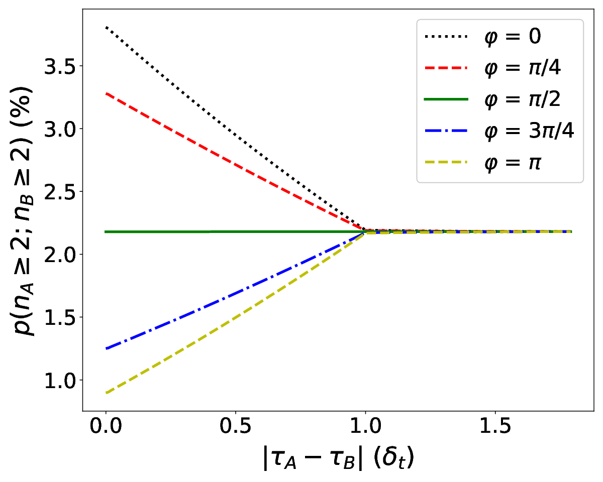
that must be discarded during key distillation Gisin_2001. The probabilities to detect exactly one photon pair and multiple photon pairs are depicted in Figs. 2 and 3, respectively, for different values of and . The remaining values are chosen to be ps, ps, based on Stucki_2006, and for the sake of simplicity. What is evident from this figure is that the interference becomes the most visible for and vanishes for increasing detuning. The probabilities converge to the constant probability pertaining to , culminating in the complete disappearance of Franson interference at a detuning of . Figure 2 reveals some very interesting conclusions. It can be inferred that linear dependence dominates the probabilities for increasing detuning, which is attributed to the convolution of two rectangle functions resulting in a triangle function. Close to the limit detuning , the probabilities indeed branch out linearly and are symmetrically distributed around the constant limit curve at . Counterintuitively, however, the curves pertaining to different values of exhibit a modest curvature, causing a substantial asymmetry compared to the constant limit curve at , which represents a non-trivial observation. Figure 3 depicts lower probabilities and a similar dependence on the detuning and . The curvature of the curves is slighter, which leads to a more symmetric distribution of the probabilities w.r.t. to the constant limit curve at than in Fig. 2. The detection of multiple photon pairs is also most likely for constructive interference since in that case the photon numbers are most strongly correlated.
These results can be used to estimate an upper bound of the detuning, such that the security of the key is not compromised. The quality of interference can be characterized by the visibility:
| (79) |
For practical QKD installations, the visibility typically amounts to at least 93 Papapanos_2020. It is well known that the visibility of Franson interference substantially depends on the mean photon number, mainly attributed to multiple photon pairs. Hence, Fig. 4 displays the visibility for different values of the detuning and the mean photon number. As one might have anticipated, the visibility decreases for higher detuning, vanishing at , and increases for lower mean photon number. Once again, the dependence on the detuning is mainly linear and exhibits a slight curvature, which decreases for lower mean photon number. To ensure the security of the key, it can be inferred that the detuning should not drop below 6.9 in the case of . This estimation represents a powerful tool to assess the impact of the detuning on Franson interference. Moreover, the mean photon number should not exceed a certain limit, even in the case of no detuning. This limit turns out to be 0.037.
VI Conclusion
In summary, a theoretical approach was presented, which provides full time-dependent counting statistics of photon pairs generated by spontaneous parametric processes in terms of efficiently computable formulas. The regime of validity is given by an arbitrarily high degree of entanglement and a low degree if the mean photon number is bounded. The counting statistics were derived for three types of time intervals, which are classified according to their widths. The joint amplitude could be chosen arbitrarily and, as communication channels, free space and fiber propagation were investigated.
Apart from direct detection of the entangled photon pairs, general setups and external influences were discussed. It was shown that the approach can be easily generalized and a general procedure to modify the derived formulas was presented. As an example of the utility of the approach, it was applied to phase-time coding and full description of Franson interference for increasing detuning of the MZIs was presented. Up to now, this could not be achieved since previous approaches did either not include all physically contributing information or not provide an efficient computation for arbitrarily high entanglement. The detection probabilities were derived to investigate this impact, revealing interesting conclusions on how Franson interference is affected by the detuning. On this basis, an acceptable range of the detuning was estimated for practical QKD installations.
The present paper is likely to motivate future studies as its regime of validity and the description of intermediate interval widths can be extended by investigating the approximations of the presented approach. Several applications of the present work can be envisaged. First, many kinds of experimental setups and external influences could be modeled and the analytic results could be compared to measurement outcomes. Secondly, the influence of noncollinear geometries and fiber coupling to counting statistics is also of appreciable interest. Finally, the assessment of the communication security of a practical QKD installation is clearly called for.

Appendix A General counting statistics
The general counting statistics in Eq. (III) are derived for one party and one spatial mode, which can be easily extended to the general result. The proof is inspired by Takeoka_2015, where a similar result has been derived for squeezed states with finite modes and the detection of zero or non-zero photons, which coincides here to the special case of . The characteristic function of an operator is given by
| (80) |
For squeezed states , this can be written as Olivares_2012
| (81) |
where denotes the covariance matrix. To address , the interval is partitioned into subintervals. Mehler’s formula Erdelyi_1995 gives
| (82) |
where denotes the projection onto . Hence, all information of the quantum state at will be eliminated. Applying the trace rule Ferraro_2005
| (83) |
for dimensions to gives
| (84) |
The limit yields the result, where becomes an operator and det denotes a Fredholm determinant.
Appendix B Proof of Theorem 1
Proof.
Here, the result concerning is derived. The idea of the proof can be easily generalized to obtain the remaining results. First of all, it can be shown that
| (85) |
satisfies , where the kernel of the integral operator is given by the JA , defined in Eq. (II). Considering powers of as
| (86) |
leads to the heart of the proof. The narrow anti-diagonal dependence of guarantees the estimation
| (87) |
for any , including and . Iterative application of this inequality gives
| (88) |
Inserting Eq. (B) in Eq. (86) suggests the approximation
| (89) |
since has normalized widths and
| (90) |
using . This yields a convolution of factors, such that applying the convolution theorem Arfken_2005 gives
| (91) |
This result can be extended to a general analytic function by expanding it as a power series. Since the proven relation, however, only holds for , higher-order terms have to be negligible. The argument of can be estimated by the maximal value . To obtain , the mean photon number can be introduced using Eqs. (23) and (24), which hold for any choice of and . ∎
References
- (1) Z. Xie, T. Zhong, S. Shrestha, X. Xu, J. Liang, Y.-X. Gong, J. C. Bienfang, A. Restelli, J. H. Shapiro, F. N. C. Wong, and C. W. Wong, Nat. Photonics 9, 536-542 (2015).
- (2) Yu. M. Mikhailova, P. A. Volkov, and M. V. Fedorov Phys. Rev. A 78, 062327 (2008).
- (3) P. Imany, J. A. Jaramillo-Villegas, O. D. Odele, K. Han, D. E. Leaird, J. M. Lukens, P. Lougovski, M. Qi, and A. M. Weiner, Opt. Express 26, 1825-1840 (2018).
- (4) C. Joshi, A. Farsi, S. Clemmen, S. Ramelow, and A. L. Gaeta, Nat. Commun. 9, 847 (2018).
- (5) B. Li, F. Hou, R. Quan, R. Dong, L. You, H. Li, X. Xiang, T. Liu, and S. Zhang, Phys. Rev. A 100, 053803 (2019).
- (6) K. Luo, S. Brauner, C. Eigner, P. R. Sharapova, R. Ricken, T. Meier, H. Herrmann, and C. Silberhorn, Sci. Adv. 5, 1 (2019).
- (7) Y. Zhai, R. Dong, B. Li, R. Quan, M. Wang, F. Hou, T. Liu, and S. Zhang, J. Phys. B: At. Mol. Opt. Phys. 50, 125502 (2017).
- (8) R. Quan, M. Wang, F. Hou, Z. Tai, T. Liu, S. Zhang, and R. Dong, Appl. Phys. B 118, 431-437 (2015).
- (9) X. Xiang, R. Dong, B. Li, F. Hou, R. Quan, T. Liu, and S. Zhang, Opt. Express 28, 17697-17707 (2020).
- (10) S. Lerch, T. Guerreiro, B. Sanguinetti, P. Sekatski, N. Gisin, and A. Stefanov, J. Phys. B: At. Mol. Opt. Phys. 50, 055505 (2017).
- (11) X. Hu, T. Zhong, F. N. C. Wong, X. Mao, P. Kharel, Z. Xie, X. Xu, C. W. Wong, and D. R. Englund, Phys. Rev. A 91, 013809 (2015).
- (12) N. Matsuda, H. Nishi, P. Karkus, T. Tsuchizawa, K. Yamada, W. J. Munro, K. Shimizu, and H. Takesue, J. Opt. 19, 124005 (2017).
- (13) M. Kues, C. Reimer, P. Roztocki, L. Cortés, S. Sciara, B. Wetzel, Y. Zhang, A. Cino, S. Chu, B. E. Little, D. J. Moss, L. Caspani, J. Azaña, and R. Morandotti, Nature 546, 622-626 (2017).
- (14) A. Martin, T. Guerreiro, A. Tiranov, S. Designolle, F. Fröwis, N. Brunner, M. Huber, and N. Gisin, Phys. Rev. Lett. 118, 110501 (2017).
- (15) C. Lee, Z. Zhang, G. R. Steinbrecher, H. Zhou, J. Mower, T. Zhong, L. Wang, X. Hu, R. D. Horansky, V. B. Verma, A. E. Lita, R. P. Mirin, F. Marsili, M. D. Shaw, S. W. Nam, G. W. Wornell, F. N. C. Wong, J. H. Shapiro, and D. Englund, Phys. Rev. A 90, 062331 (2014).
- (16) S. Arahira and H. Murai, Jpn. J. Appl. Phys. 55 032801 (2016).
- (17) J. Brendel, N. Gisin, W. Tittel, and H. Zbinden, Phys. Rev. Lett. 82, 2594 (1999).
- (18) D. Stucki, H. Zbinden, and N. Gisin, Journal of Modern Optics 52(18), 2637 (2006).
- (19) N. Gisin, G. Ribordy, W. Tittel, and H. Zbinden, Rev. Mod. Phys. 74, 145 (2001).
- (20) H.-P. Lo, T. Ikuta, N. Matsuda, T. Honjo, W. J. Munro, and H. Takesue, Phys. Rev. Appl. 13, 034013 (2020).
- (21) M. Pavicic, Phys. Lett. A 380, 848-855 (2016).
- (22) A. C. Peacock and M. J. Steel, Science 351 (6278), 1152 (2016).
- (23) C. Müller, A. Ahlrichs, and O. Benson, Phys. Rev. A 102, 053504 (2020).
- (24) L. Gao, Y. Zhang, E. Cohen, A. C. Elitzur, and E. Karimi Appl. Phys. Lett. 115, 051102 (2019).
- (25) H. Takesue and K. Shimizu, Opt. Comm. 283, 276-287 (2010).
- (26) P.-S. Yan, L. Zhou, W. Zhong, and Y.-B. Sheng, Opt. Express 29(2), 571-583 (2021).
- (27) T. Ikuta and H. Takesue, Phys. Rev. A 93, 022307 (2016).
- (28) M. Takeoka, R.-B. Jin, and M. Sasaki, New J. Phys. 17, 043030 (2015).
- (29) D. Richart, Y. Fischer, and H. Weinfurter, Appl. Phys. B 106, 543-550 (2012).
- (30) F. Hou, X. Xiang, R. Quan, M. Wang, Y. Zhai, S. Wang, T. Liu, S. Zhang, and R. Dong, Appl. Phys. B 122, 128 (2016).
- (31) S. P. Phehlukwayo, M. L. Umuhire, Y. Ismail, S. Joshi, and F. Petruccione, Phys. Rev. A 102, 033732 (2020).
- (32) H. Liu and A. S. Helmy, npj Quantum Inf. 6, 66 (2020).
- (33) K. E. Dorfman, S. Asban, B. Gu, and S. Mukamel, Commun. Phys. 4, 49 (2021).
- (34) J. M. Lukens, A. Dezfooliyan, C. Langrock, M. M. Fejer, D. E. Leaird, and A. M. Weiner, Opt. Lett. 38, 4652-4655 (2013).
- (35) Z. Zhang, C. Yuan, S. Shen, H. Yu, R. Zhang, H. Wang, H. Li, Y. Wang, G. Deng, Z. Wang, L. You, Z. Wang, H. Song, G. Guo, and Q. Zhou, npj Quantum Inf 7, 123 (2021).
- (36) C. E. Kuklewicz, Ph.D. thesis, Massachusetts Institute of Technology (2005).
- (37) M. Wang, F. Yan, and T. Gao, J. Phys. B: At. Mol. Opt. Phys. 53, 135503 (2020).
- (38) E. Brambilla, A. Gatti, M. Bache, and L. A. Lugiato, Phys. Rev. A 69, 023802 (2004).
- (39) S. Signorini and L. Pavesi, AVS Quantum Sci. 2, 041701 (2020).
- (40) W. Mauerer, M. Avenhaus, W. Helwig, and C. Silberhorn, Phys. Rev. A 80, 053815 (2009).
- (41) I. A. Burenkov, A. K. Sharma, T. Gerrits, G. Harder, T. J. Bartley, C. Silberhorn, E. A. Goldschmidt, and S. V. Polyakov, Phys. Rev. A 95, 053806 (2017).
- (42) L. Lamata and J. León, J. Opt. B: Quantum Semiclass. Opt. 7, 224-229 (2005).
- (43) C. K. Law and J. H. Eberly, Phys. Rev. Lett. 92, 127903 (2004).
- (44) Jan Peřina, Jr., Phys. Rev. A 93, 063857 (2016).
- (45) F. Xu, X. Ma, Q. Zhang, H.-K. Lo, and J.-W. Pan, Rev. Mod. Phys. 92, 025002 (2020).
- (46) J. K. Nauth, MSc Thesis, Technical University of Darmstadt (2020).
- (47) J. Schneeloch and J. C. Howell, J. Opt. 18, 053501 (2016).
- (48) Z. Y. Jeff Ou, Multi-photon Quantum interference (Springer Science+Business Media LLC, New York, 2007), p. 25-26.
- (49) K. Garay-Palmett, M. Corona, and A. U’Ren, Rev. Mex. Fis. S 57, 3 (2011).
- (50) C.-Y. Yang, C. Lin, C. Liljestrand, W.-M. Su, C. Canalias, and C.-S. Chuu, Sci Rep 6, 26079 (2016).
- (51) J. Schneeloch, S. H. Knarr, D. F. Bogorin, M. L. Levangie, C. C. Tison, R. Frank, G. A. Howland, M. L. Fanto, and P. M. Alsing, J. Opt. 21, 043501 (2019).
- (52) N. Quesada and J. E. Sipe, Phys. Rev. A 90, 063840 (2014).
- (53) S. Blanes, F. Casas, J. A. Oteoc, and J. Ros, Phys. Rep. 470, p. 151-238 (2009).
- (54) G. Molina-Terriza, S. Minardi, Y. Deyanova, C. I. Osorio, M. Hendrych, and Juan P. Torres, Phys. Rev. A 72, 065802 (2005).
- (55) E. Toninelli, Ph.D. thesis, University of Glasgow, 2020.
- (56) L. Zhang, C. Silberhorn, and I. A. Walmsley, Phys. Rev. Lett. 100, 110504 (2008).
- (57) L. Mandel and E. Wolf, Optical Coherence and Quantum Optics (Cambridge University Press, Cambridge, 1995), p. 725.
- (58) N. L. Johnson, A. W. Kemp, and S. Kotz, Univariate Discrete Distributions (John Wiley & Sons, New Jersey, 2005), 3rd ed., p. 58-60.
- (59) S. P. Walborn, C. H. Monken, S. Pádua, P. H. Souto Ribeiro, Phys. Rep. 495, p. 87-139 (2010).
- (60) F. Bornemann, Math. Comp. 79 (2010), pp. 871-915.
- (61) M. G. A. Paris, Phys. Lett. A 289, 167 (2001).
- (62) A. Ferraro, S. Olivares, and M. G. A. Paris, Gaussian States in Quantum Information (Napoli Series on physics and Astrophysics, Bibliopolis, 2005), p. 43.
- (63) X. Ma and W. Rhodes, Phys. Rev. A 41, 4625 (1990).
- (64) S. Olivares, Eur. Phys. J. Special Topics 203, 3 (2012).
- (65) C. Papapanos, D. Zavitsanos, A. Raptakis, G. Giannoulis, C. Kouloumentas, and H. Avramopoulos, Eur. Phys. J. D 75, 93 (2021).
- (66) A. Erdélyi, W. Magnus, F. Oberhettinger, and F. Tricomi, Higher transcendental functions (McGraw-Hill, California, 1953), Vol. 2, p. 194.
- (67) G. B. Arfken and H. J. Weber, Mathematical Methods for Physicists (Academic Press, Oxford, 2005), 6th ed., p. 951-952.