The nonlinear Klein-Gordon equation on metric graphs: Modeling reflectionless transmission of the kink soliton

Asadov Q.U.* Sabirov K.K.** Aripov M.*** Affiliation: *, ** Tashkent university of information technologies named after Al-Khwarizmi Affiliation: Dept. Algoritmization and mathematical modelling Affiliation: *** National University of Uzbekistan named after Mirzo Ulugbek Affiliation: Dept. Applied mathematics and computer analysis Affiliation: Tashkent, Uzbekistan

August 11, 2026

Abstract

In this paper we consider the nonlinear Klein-Gordon equation on the metric star graph with tree semi-infinite bonds. At the branched point we put two types of vertex boundary conditions: the weight continuity and the condition for derivatives of wave functions as the generalized Kirchhoff rule. We solve this equation satisfying vertex boundary conditions and the energy, momentum conservation laws. We also show reflectionsless propagations of the kink soliton solution, plot the reflection coefficient and extend to other topologies.

1 Introduction

Nonlinear dynamics of solitary waves, that occur in many scientific areas, can be described by nonlinear partial differential equations [1], [2]. The nonlinear Klein-Gordon equation is one of the important classes of partial differential equations and is used to model many different phenomena, including the propagation of dislocations in crystals and the behavior of elementary particles [3]. The exact and numerical soliton solutions of Klein-Gordon equation are given in the pioneer work [4], in that numerically solved with the time and coordinate steps $k=h=0.05$ and found the descritization scheme using Taylor series. The energy and momentum conservating schemes used to integrate the nonlinear Klein-Gordon equation in [5] and invariant-conserving finite difference algorithms are given in [6].

The nonlinear partial differential equations on the branched structures are attached the most interest in the last decade years. Such attention was caused by the possibility for obtaining soliton solution of nonlinear partial differential equations such as nonlinear Schrödinger, Dirac equations and its numerous applications in different branches of physics [7, 8, 9, 10, 11]. The branched structures can be modeled metric graphs. Metric graphs are consist of two sets: the set of points (vertices) and the set of intervals that connect vertices. Topology of graphs can be given so called adjacency matrices [12, 13]:

C_{ij}=\left\{\begin{array}[]{ll}1,\,i,j\text{ are connected,}\\ 0,\,\text{otherwise,}\end{array}\right.i,j=1,2,...,V

In this paper we focus on one of the exact solutions and transmission of the kink soliton of the nonlinear Klein-Gordon equation through the vertices of the networks. The present work is organized as follows: in the section 2 the nonlinear Klein-Gordon equation on the metric star graph with derivations the vertex boundary conditions is obtained; in the section 3 the kink soliton solution of the formulated problem with the sum rule for the reflectionless transmission is analytically given, the momentum conservation law is shown constant and plotted the energy conservation law with the plotting reflection coefficient as the ratio of momentums; the section 4 is devoted for the extensions to other topologies of metric graphs such as the tree and loop graphs; in the last section the conclusions are given.

2 Formulation of the problem

We consider a star graph with three bonds $e_{j}$ , for which a coordinate $x_{j}$ is assigned. Choosing the origin of coordinates at the vertex, 0, for bond $e_{1}$ we put $x_{1}\in(-\infty,0]$ and for $e_{2,3}$ we fix $x_{2,3}\in[0,+\infty)$ . In what follows, we use the shorthand notation $q_{j}(x)$ for $q_{j}(x_{j})$ where $x$ is the coordinate on the bond $j$ to which the component $q_{j}$ refers. Klein-Gordon equation on the each bond $e_{j}$ of the star graph is written as

\partial_{tt}^{2}q_{j}-\partial_{xx}^{2}q_{j}-q_{j}+b_{j}q_{j}^{3}=0.

(1)

Refer to caption — Figure 1: The metric star graph

Now we define the vertex boundary conditions at the branched point of the star graph, therefore we derive these boundary conditions from conservation laws. One of the conservation laws is energy. The energy conservation law is defined as

E=\sum_{j=1}^{3}E_{j},

(2)

where

E_{j}=\int_{e_{j}}\left[\frac{1}{2}(\partial_{t}q_{j})^{2}+\frac{1}{2}(\partial_{x}q_{j})^{2}-\frac{1}{2}q_{j}^{2}+\frac{b_{j}}{4}q_{j}^{4}\right]dx.

(3)

From $\dot{E}=0$ we can get the following nonlinear boundary condition as

\partial_{x}q_{1}\partial_{t}q_{1}|_{x=0}=\partial_{x}q_{2}\partial_{t}q_{2}|_{x=0}+\partial_{x}q_{3}\partial_{t}q_{3}|_{x=0}.

(4)

We need two types of boundary conditions to find a solution of (1) and to fulfil the nonlinear vertex boundary condition (4). Therefore the first type of vertex boundary conditions is the following weight continuity

\alpha_{1}q_{1}|_{x=0}=\alpha_{2}q_{2}|_{x=0}=\alpha_{3}q_{3}|_{x=0},

(5)

the second type of vertex boundary conditions is given derivatives of wave functions at the branched point as Kirchhoff rule

\frac{1}{\alpha_{1}}\partial_{x}q_{1}|_{x=0}=\frac{1}{\alpha_{2}}\partial_{x}q_{2}|_{x=0}+\frac{1}{\alpha_{3}}\partial_{x}q_{3}|_{x=0}.

(6)

3 The kink soliton solution of Klain-Gordon equation on the star graph with three edges

The kink (antikink) soliton solution of Klein-Gordon equation (1) on the each bond $e_{j}$ of the metric star graph is the following

q_{j}(x,t)=\mp\frac{1}{\sqrt{b_{j}}}\,{\rm tanh}\left(\frac{x-l-\upsilon t}{\sqrt{2(1-\upsilon^{2})}}\right),

(7)

where $l$ is the initial center of mass of soliton (the kink and antikink soliton solutions are with the signs $-$ and $+$ , respectively). Fulfilling the vertex boundary conditions (5)-(6) we can get the following constrains

	$\displaystyle\frac{\alpha_{1}}{\sqrt{b_{1}}}=\frac{\alpha_{2}}{\sqrt{b_{2}}}=\frac{\alpha_{3}}{\sqrt{b_{3}}},$		(8)
	$\displaystyle\frac{1}{\alpha_{1}\sqrt{b_{1}}}=\frac{1}{\alpha_{2}\sqrt{b_{2}}}+\frac{1}{\alpha_{3}\sqrt{b_{3}}}.$		(9)

From Eq.s(8) and (9) we obtain the following sum rule for nonlinearities

\frac{1}{b_{1}}=\frac{1}{b_{2}}+\frac{1}{b_{3}}.

(10)

Using the kink (antikink) soliton solution of Klein-Gordon equation (1) with the sum rule for the nonlinearities (10) we can also show that another conservation law, i.e. the momentum is conserved:

P=\sum_{j=1}^{3}\int_{e_{j}}\partial_{t}q_{j}\partial_{x}q_{j}dx=\sum_{j=1}^{3}\frac{1}{2b_{j}}\cdot\frac{\upsilon}{1-\upsilon^{2}}\int_{e_{j}}\frac{dx}{cosh^{4}\left(\frac{x-l-\upsilon t}{\sqrt{2(1-\upsilon^{2})}}\right)}=

=\frac{\upsilon}{2(1-\upsilon^{2})}\left[\frac{1}{b_{1}}\int_{-\infty}^{0}\frac{dx}{cosh^{4}\left(\frac{x-l-\upsilon t}{\sqrt{2(1-\upsilon^{2})}}\right)}+\left(\frac{1}{b_{2}}+\frac{1}{b_{3}}\right)\int_{0}^{+\infty}\frac{dx}{cosh^{4}\left(\frac{x-l-\upsilon t}{\sqrt{2(1-\upsilon^{2})}}\right)}\right]=

=\frac{\upsilon}{2(1-\upsilon^{2})b_{1}}\int_{-\infty}^{+\infty}\frac{dx}{cosh^{4}\left(\frac{x-l-\upsilon t}{\sqrt{2(1-\upsilon^{2})}}\right)}=\frac{4\upsilon}{3b_{1}\sqrt{2(1-\upsilon^{2})}},

from the last expression the momentum is constant.

In the figure 2 the propagation of the kink soliton solution from the first bond to the second and third bonds is plotted and the refletionless transmission is shown at $t=0,\,t=5$ and $t=10$ . In the figure 3 it is plotted the energies on the each bonds and the total energy, from this figure it is clear seen that the total energy is constant. The reflection coefficient $R(b_{3},t=10)=\frac{P_{1}(t=10)}{P_{1}(t=10)+P_{2}(t=10)+P_{3}(t=10)}$ is plotted as a function of $b_{3}$ for fixed $b_{j},\,j=1,2,\,\alpha_{1},\,\alpha_{2},\,\alpha_{3}=\frac{1}{\sqrt{b3}\left(\frac{1}{\alpha_{3}\sqrt{b3}}-\frac{1}{\alpha_{2}\sqrt{b2}}\right)}$ . This systematic analysis clearly illustrates the necessity for reflection to be absent at $b_{3}=3$ .

4 Extensions to other topologies of metric graphs

The above approach of the nonlinear Klein-Gordon equation on the metric star graph can be extended to the tree graph presented in figure 5. This tree graph consists of three subgraphs $e_{1}\sim(-\infty;0],\,e_{1i}\sim[0;L_{i}]$ and $e_{1ij}\sim[0;+\infty)$ , where $i,j=1,2$ . On the each bond we consider the nonlinear Klein-Gordon equation as given by

\partial_{tt}^{2}q_{e}-\partial_{xx}^{2}q_{e}-q_{e}-b_{e}q_{e}^{3}=0,

(11)

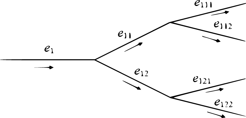
with the following boundary conditions at the vertices

\displaystyle\left\{\begin{array}[]{ll}\alpha_{1}q_{1}|_{x=0}=\alpha_{11}q_{11}|_{x=0}=\alpha_{12}q_{12}|_{x=0};\\ \frac{1}{\alpha_{1}}\partial_{x}q_{1}|_{x=0}=\frac{1}{\alpha_{11}}\partial_{x}q_{11}|_{x=0}+\frac{1}{\alpha_{12}}\partial_{x}q_{12}|_{x=0}.\\ \alpha_{11}q_{11}|_{x=L_{1}}=\alpha_{111}q_{111}|_{x=0}=\alpha_{112}q_{112}|_{x=0};\\ \frac{1}{\alpha_{11}}\partial_{x}q_{11}|_{x=L_{1}}=\frac{1}{\alpha_{111}}\partial_{x}q_{111}|_{x=0}+\frac{1}{\alpha_{112}}\partial_{x}q_{112}|_{x=0}.\\ \alpha_{12}q_{12}|_{x=L_{2}}=\alpha_{121}q_{121}|_{x=0}=\alpha_{122}q_{122}|_{x=0};\\ \frac{1}{\alpha_{12}}\partial_{x}q_{12}|_{x=L_{2}}=\frac{1}{\alpha_{121}}\partial_{x}q_{121}|_{x=0}+\frac{1}{\alpha_{122}}\partial_{x}q_{122}|_{x=0}.\\ \end{array}\right.

The kink (antikink) soliton solution of equation (11) can be written as

q_{e}(x,t)=\mp\frac{1}{\sqrt{b_{e}}}\,{\rm tanh}\left(\frac{x-x_{0,e}-\upsilon t}{\sqrt{2(1-\upsilon^{2})}}\right).

(19)

where

x_{0,1}=x_{0,11}=x_{0,12}=l,\,x_{0,111}=x_{0,112}=l-L_{1},\,x_{0,121}=x_{0,122}=l-L_{2}.

(20)

$l-$ initial center of the mass of solution. Satisfying the boundary conditions (4) we have the following sum rules for nonlinearities

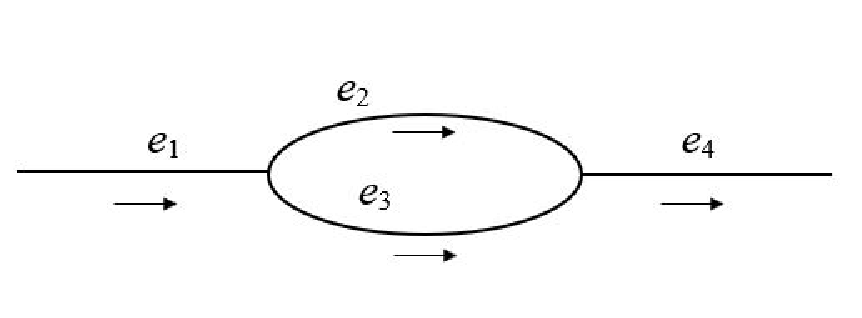
\displaystyle\left.\begin{array}[]{lll}\frac{1}{b_{1}}=\frac{1}{b_{11}}+\frac{1}{b_{12}},\\ \frac{1}{b_{11}}=\frac{1}{b_{111}}+\frac{1}{b_{112}},\\ \frac{1}{b_{12}}=\frac{1}{b_{121}}+\frac{1}{b_{122}}.\end{array}\right.

Now we consider the loop graph plotted in figure 6 with subgraphs $e_{1}\sim(-\infty;0],\,e_{2},e_{3}\sim[0;L]$ and $e_{4}\sim[L;+\infty)$ . On the each bond of this loop graph the nonlinear Klein-Gordon equation can be written by equation (11) with the boundary conditions at the vertices

\left\{\begin{array}[]{ll}\alpha_{1}q_{1}|_{x=0}=\alpha_{2}q_{2}|_{x=0}=\alpha_{3}q_{3}|_{x=0};\\ \frac{1}{\alpha_{1}}\partial_{x}q_{1}|_{x=0}=\frac{1}{\alpha_{2}}\partial_{x}q_{2}|_{x=0}+\frac{1}{\alpha_{3}}\partial_{x}q_{3}|_{x=0}.\\ \alpha_{2}q_{2}|_{x=L}=\alpha_{3}q_{3}|_{x=L}=\alpha_{4}q_{4}|_{x=0};\\ \frac{1}{\alpha_{2}}\partial_{x}q_{2}|_{x=L}+\frac{1}{\alpha_{3}}\partial_{x}q_{3}|_{x=L}=\frac{1}{\alpha_{4}}\partial_{x}q_{4}|_{x=0}.\end{array}\right.

(25)

The kink (antikink) soliton solution is given by equation (19), where $x_{0,1}=x_{0,2}=x_{0,3}=l,\,x_{0,4}=l-L$ . Satisfying the boundary conditions (25) we can get the sum rule written as

\displaystyle\left.\begin{array}[]{ll}\frac{1}{b_{1}}=\frac{1}{b_{2}}+\frac{1}{b_{3}}=\frac{1}{b_{4}}.\end{array}\right.

5 Conclusions

In this paper we studied the nonlinear Klein-Gordon equation on the simplest metric graphs as the star graph with tree semi-infinite bonds, tree and loop graphs. First of all we derived the nonlinear boundary condition from the energy conservation law. Satisfying this boundary conditions at the vertex (branched point) we obtained the weight continuity and the condition for derivatives of the wave function as Kirchhoff rule. We obtained the soliton solution on the metric star graph and the constrain as inverses of nonlinearities for the reflectionless transmission. Using the soliton solution we got that the total momentum is conserved. We showed the conservation of the total energy and calculated the reflection coefficient as the ratio of the momentum on the first bond to the total momentum in the figures 3 and 4, respectively. We also extended obtained results as the formulation problems and the constrains for the nonlinearities to the tree and loop graphs.

References

[1] Ablowitz M.J. and Segur H., Solitons and the Inverse Scattering Transform, Philadelphia, 1981.
[2] Ablowitz M.J., Clarkson P.A., Solitons, Nonlinear Evolution Equations and Inverse Scattering, Cambridge University Press 1991.
[3] Greiner W., Relativistic Quantum Mechanics-Wave Equations, Springer-Verlag, Berlin, Germany, 3rd edition, 2000.
[4] Ablowitz M.J., Kruskal M.D. and Ladik J.F., Solitary wave collisions SIAM J. Appl. Math. Vol. 36, No. 3, June 1979
[5] Jiménez S.,Vázquez L., Analysis of Four Numerical Schemes for a Nonlinear Klein-Gordon Equation, App. Math. and Comp.35:61-94 (1990)
[6] Los Vu-Quos and Shaofan Li, Invariant-conserving finite difference algorithms for the nonlinear Klein-Gordon equation, Computer Methods in Applied Mechanics and Engineering 107 (1993) 341-391. North-Holland, CMA 403
[7] Sobirov Z., Matrasulov D., Sabirov K., Sawada S. and Nakamura K., Integrable nonlinear Schrödinger equation on simple networks: Connection formula at vertices, PHYSICAL REVIEW E 81: 066602 (2010)
[8] Adami R., Cacciapuoti C., Finco D. and Noja D., Fast solitons on star graphs, Reviews in Mathematical Physics, Vol. 23, No. 4, 409–451 (2011)
[9] Sobirov Z., Babajanov D., Matrasulov D., Nakamura K. and Uecker H., Sine-Gordon solitons in networks: Scattering and transmission at vertices, EPL, A letters journal exploring the frontiers of physics, 115, 50002 (2016)
[10] Sabirov K.K., Babajanov D.B., Matrasulov D.U. and Kevrekidis P.G., Dynamics of dirac solitons in networks, J. Phys. A: Math. Theor. 51, 435203 (2018)
[11] Sabirov K.K., Yusupov J.R., Matyokubov Kh.Sh., Susanto H., Matrasulov D.U., Networks with point-like nonlinearities, Nanosystems: Phys. Chem. Math., 13(1), 30–35. (2022)
[12] Kottos T. and Smilansky U., Periodic Orbit Theory and Spectral Statistics for Quantum Graphs, (2008)
[13] Gnutzmann S. and Smilansky U., Quantum graphs: Applications to quantum chaos and universal spectral statistics, Advances in Physics, Vol. 55, Nos. 5–6, July–October, 527–625. (2006)