We extend results known for the randomized Gauss-Seidel and the Gauss-Southwell methods for the case of a Hermitian and positive definite matrix to certain classes of non-Hermitian matrices. We obtain convergence results for a whole range of parameters describing the probabilities in the randomized method or the greedy choice strategy in the Gauss-Southwell-type methods. We identify those choices which make our convergence bounds best possible. Our main tool is to use weighted -norms to measure the residuals. A major result is that the best convergence bounds that we obtain for the expected values in the randomized algorithm are as good as the best for the deterministic, but more costly algorithms of Gauss-Southwell type. Numerical experiments illustrate the convergence of the method and the bounds obtained. Comparisons with the randomized Kaczmarz method are also presented.
MSC Classification]15A06, 65F15
On the Convergence of Randomized and Greedy Relaxation Schemes for Solving Nonsingular Linear Systems of Equations
keywords
Randomized Gauss-Seidel. Convergence bounds. Greedy algorithms. Gauss-Southwell algorithm. Randomized smootherpacs
[1 Introduction
Classical stationary iterations such as Jacobi and Gauss-Seidel (see, e.g., Berman and Plemmons 1994; Saad 1996; Varga 1962) to solve a square linear system
| (1) |
nowadays are found to be useful in many situations, such as smoothers for multigrid methods (see, e.g.,Rüde 1993; Trottenberg et al. 2000), in high performance computing (see, e.g., Wolfson-Pou and Chow 2017) and in particular as scafolding for methods for discretized PDEs based on domain decomposition; see, e.g., Glusa et al. 2020; Magoulès et al. 2017; Smith et al. 1996.
In recent years, randomized algorithms have gained a lot of attention in numerical computation; see, e.g., the surveys Kannan and Vempala 2017 and Martinsson and Tropp 2020. Many different randomized methods and algorithms have in particular been suggested and analyzed for the solution of consistent and non-consistent, square and non-square linear systems; see, e.g., Gower and Richtárk 2015. These methods are attractive in situations which typically arise in an HPC or a data science context when matrix products are considerably expensive or when the matrix is so large that it does not fit in main memory; see, e.g., the discussion in the recent paper Gower et al. 2021.
For linear systems, the emphasis has been so far on randomized coordinate descent type algorithms. These methods aim at finding the minimizer of a convex functional , the minimizer being the solution of the linear system. The methods perform a sequence of relaxations, where in each relaxation a coordinate is chosen at random and the current iterate is modified to become the -th unit vector and such that is minimal. Many convergence results on randomized coordinate descent methods are known, see Gower and Richtárk 2015; Richtárik and Takáč 2020, e.g., and the typical assumption is that is at least differentiable.
If in (1) is Hermitian and positive definite (hpd), and we take , minimizing in coordinate is equivalent to solving equation of (1) with respect to . The resulting randomized coordinate descent method is thus a randomized version of the Gauss-Seidel method, and an analysis of this randomized method was given in Leventhal and Lewis 2010 and also, in the more general context of randomized Schwarz methods in Hilbert spaces, in Griebel and Oswald 2012. See also Avron et al. 2015.
If in (1) is not hpd, the typical approach is to obtain a randomized algorithm is to consider randomized Kaczmarz methods, i.e., coordinate descent for one of the normal equations or with corresponding convex and differentiable functionals and , respectively. This approach can also be pursued when is non-square, and the system may be consistent or non-consistent. Note that the original Kaczmarz method Kaczmarz 1937 corresponds to coordinate descent for with an integrated back-transformation from the iterate to . We emphasize that while coordinate descent for is often also termed “Gauss-Seidel”, it is different from classical Gauss-Seidel directly applied to (1), which is what we focus on in this paper. There is a tremendous amount of literature dealing with randomized Kaczmarz type algorithms which we cannot cite exhaustively here. Recent publications include Bai and Wu 2018a; Bai and Wu 2018b; Bai and Wu 2021; Bai et al. 2021; Bai et al. 2022; Du 2019; Gower et al. 2021; Guan et al. 2020; Guo and Li 2018; Haddock and Ma 2021; Ma et al. 2015; Steinerberger 2021a; Steinerberger 2021b; Wang et al. 2022; Yang 2021.
Now, when is square and non-singular, considering a randomized version of the Gauss-Seidel method applied to the linear system (1) directly, is an attractive alternative to the randomized Kaczmarz type approaches, since under appropriate conditions on it converges more rapidly and requires less work per iteration. This is known to be the case when is hpd; see the papers Leventhal and Lewis 2010 and Griebel and Oswald 2012 mentioned earlier. The main new contribution of the present work is a convergence analysis for randomized Gauss-Seidel also for the case when is generalized diagonally dominant. An important methodological aspect of our work is that for generalized diagonally dominant we do not directly relate Gauss-Seidel for (1) to an equivalent coordinate descent method for an appropriate convex functional. Our technique of proof will, nevertheless, rely on showing that the iterates reduce—but, as opposed to gradient descent, do not necessarily minimize—a weighted -norm of the residual . Note that -norms are not differentiable and that weighted (and ) -norms) arise canonically in the context of generalized diagonal dominance; see, e.g., Berman and Plemmons 1994; Varga 1962. As a ‘by-product” of our analysis, we will also obtain convergence results of greedy choice algorithms of Gauss-Southwell type, see below.
In this paper, we consider general methods based on a splitting so that with and one obtains the (affine) fixed point iteration
| (2) |
as an iterative solution method for . In particular, the solution of (1) is a fixed point of (2). Usually, the matrix is never formed. Instead, a linear system with the coefficient matrix is solved at each iteration . In this general splitting framework, the Gauss-Seidel method is characterized by being the lower triangular part of , and the method is equivalent to relaxing one row at a time in the natural order . In other terms, if we write the classical Jacobi splitting , being the diagonal of , then, with , we have the following rendition of the Gauss-Seidel algorithm, using a “global” index for each single relaxation.
Each update from to is termed one relaxation, and such relaxations, since they are done one after the other, correspond to one iteration in (2) with , where and denote the lower and upper triangular part of , respectively (and . So, successive relaxations of a “Jacobi-type”, i.e. with , performed in the natural order , is identical to one iteration of Gauss-Seidel.
Gauss in fact proposed another method, later popularized by Southwell, and known either as Southwell method or as Gauss-Southwell method; see, e.g., the historic review of these developments in Saad 2020. We describe this method in Algorithm 2 for a general splitting based method where with . The Gauss-Southwell method arises for . The original Gauss-Southwell method selects the component to be relaxed as the one at which the residual is largest, i.e., it takes for which
| (3) |
As a consequence, we are not updating components in a prescribed order, but rather choose the row to relax to be the one for which the current residual has its largest component. This can be considered a greedy pick strategy, and we formulate Algorithm 2 in a manner to allow for general greedy pick rules.
A generalization of the greedy pick rule (3) is to fix weights and choose such that
| (4) |
blue cf. Griebel and Oswald 2012, and we will see later that for appropriate choices of the we can prove better convergence bounds than for the standard greedy pick rule (3).
Both greedy pick rules (3) and (4) require an update of the residual after each relaxation, which represents extra work. Moreover, additional work is required for computing the maximum. Using the “preconditioned” residual can to some extent reduce this overhead: Once is computed, the next relaxation can be obtained easily as
We might therefore want to use a greedy pick rule based on the preconditioned residuals, which using fixed weights as before, can be formulated as
| (5) |
It has been demonstrated that Gauss-Southwell can indeed converge in fewer relaxations than Gauss-Seidel, but the total computational time is often higher, due to the computation of the maximum, and, in a parallel setting, the added cost of communication Wolfson-Pou and Chow 2017.
In this paper, we discuss the greedy relaxation scheme of Algorithm 2 as well as a randomized version of Algorithm 1, which for is usually called randomized Gauss-Seidel. We give bounds on the expected value of the residual norm which match analogous convergence bounds for the greedy algorithm.
The randomized iteration derived from (2) fixes probabilities , , with and proceeds as follows.
In the randomized Algorithm 3, the order of the relaxation does not follow a prescribed order, as in Gauss-Seidel, nor a greedy order depending on the entries in the current residual vector, as in Gauss-Southwell, but instead, each row to relax is chosen at random with a fixed positive probability .
The paper is organized as follows. We first repeat the convergence results from Griebel and Oswald 2012; Leventhal and Lewis 2010 for matrices which are hpd in Section 2, and then, in the rest of the paper, present new results for non-Hermitian matrices. As a byproduct of our investigation, we also show that some greedy choices other than (3) produce methods for which we obtain better bounds on the rate of convergence.
Our results are theoretical in nature and illustrated with numerical experiments. We are aware that other methods may be more efficient than those discussed here. But we believe that our results represent an interesting contribution to randomized and greedy relaxation algorithms since they show that we can deviate from the slowly converging Kaczmarz type approaches not only when is hpd but also when is (generalized) diagonally dominant. We thus trust that on one hand, the results are interesting in and on themselves, and on the other they may form the basis for the analysis of other practical methods. Asynchronous iterative methods Frommer and Szyld 2000, for example, can be interpreted in terms of randomized iterations; see, e.g., Avron et al. 2015; Strikwerda 2002. We expect that the theoretical tools developed here can also serve as a foundation for the analysis of such asynchronous methods, as well as for randomized block methods and randomized Schwarz methods for nonsingular linear systems; cf. Griebel and Oswald 2012.
For future use we recall that where is the solution of the linear system (1) and is the error at the relaxation (or iteration) .
2 The Hermitian and positive definite case
Consider the particular case that in Algorithms 2 and 3 arises from the (relaxed) Jacobi splitting
| (6) |
where is a relaxation parameter, i.e.
| (7) |
Then the fixed point iteration (2) is just the relaxed Jacobi iteration, which reduces to standard Jacobi if , and the associated randomized iteration from Algorithm 3 is the randomized relaxed Gauss-Seidel method whereas the associated greedy Algorithm 2 is known as the relaxed Gauss-Southwell method if we take the greedy pick rule (3). Using the residual , the update in the third lines of Algorithms 2 and 3 for can alternatively be formulated as
| (8) |
where denotes the th canonical unit vector in .
Now assume that is hpd. The Jacobi iteration then does not converge unconditionally, a sufficient condition for convergenc being that with the matrix is hpd as well. The relaxed Gauss-Seidel iteration, on the other hand, is unconditionally convergent provided ; see, e.g., Varga 1962.
For the randomized Gauss-Seidel and the Gauss-Southwell iterations the following results are essentially known.
In fact, most of Theorem 2 is a special case of what was shown in Leventhal and Lewis 2010 and Griebel and Oswald 2012 in the fairly more general context of (relaxed) randomized multiplicative Schwarz methods. For the sake of completeness, and to set the stage for our new results, we repeat the essentials of the proofs in Leventhal and Lewis 2010 and Griebel and Oswald 2012 here.
We use the -inner product and the -energy norm which, for hpd, are defined as
with the standard inner product on . Before we state the main theorem, we formulate the following useful result relating the harmonic and the arithmetic means of a sequence and the extrema of the product sequence.
Lemma 1.
Let with , . Then
where
are the harmonic mean and the arithmetic mean, respectively.
Proof.
Take the special convex combination of the with coefficients . Then , and for the convex combination of the with coefficients there is at least one index, say , for which , since otherwise for all and thus . This proves . The inequality for the minimum follows in a similar manner. ∎
Theorem 2.
Let be hpd and denote its smallest eigenvalue.
- (i)
- (ii)
Proof.
If in relaxation we choose to update component , then
| (13) | |||||
| (14) |
Therefore, in randomized Gauss-Seidel the expected value for , conditioned to the given value for , is
with the last inequality holding due to . This gives (9). If we have , then , and this is larger or equal than for any choice of the probabilities by Lemma 1. This gives the second statement in part (i).
We note that if in randomized Gauss-Seidel we choose all probabilities to be equal, for all , then
in (9), which is smaller than unless all diagonal elements are equal. We have a completely analogous situation for Gauss-Southwell: If we take the unweighted greedy pick rule (3), we obtain a value for which, interestingly, is the same than for randomized Gauss-Seidel with uniform probabilities. And this value is smaller than the value that we obtain for the weighted greedy pick rule (12), a value which is, interestingly again, equal what we obtain as the maximum value for in the randomized method (with the weighted probabilities ).
Note also that if one scales the hpd matrix symmetrically so that it has unit diagonal, then the greedy pick (12) in Theorem 2 (ii) reduces to the standard Gauss-Southwell pick (3): Let , then, the system (1) is equivalent to with the change of variables . Running Algorithm 2 for and in the variables with the greedy pick (4) with is equivalent to running the same algorithm for and in the variables with the standard greedy pick (3). One can then express the bounds of the theorem in the scaled variables in the appropriate energy norm, since we have cf. (Avron et al. 2015, Section 3.1).
Numerical example
Throughout this paper we give illustrative numerical examples based on the convection-diffusion equation for a concentration
| (15) | |||||
The positive diffusion coefficients and are allowed to depend on and , , and this also holds for the velocity field . We discretize in space using standard finite differences with interior equispaced grid points in each direction. This leaves us with the semi-discretized system
where now is a two-dimensional array, each component corresponding to one grid point. Using the implicit Euler rule as a symplectic integrator means that at a given time and a stepsize we have to solve
| (16) |
for . We illustrate the covergence behavior of the Gauss-Seidel variants considered in this paper when solving the system (16) for appropriate choices of and .
Since Theorem 2 deals with the hpd case, we now assume that there is no convection, . Then is the discretization of the diffusive term using central finite differences and as such it is an irreducible diagonally dominant M-matrix and thus hpd; see, e.g., Berman and Plemmons 1994. Accordingly, is hpd as well. We took which gives a spacing of , and and we consider two cases: constant diffusion coefficients
| (17) |
which gives a constant diagonal in , and non-constant diffusion coefficients
| (18) |
which makes the entries on the diagonal of vary between and , i.e., between 2 and 9.5.
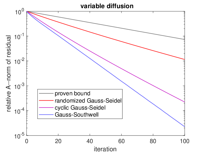
Figure 1 reports the numerical results. We chose the right hand side in (16) as , where is the discretized evaluation of the function . So we know the exact solution, which allows us to report -norms of the error, which is what we provided bounds for in Theorem 2. The figure displays these -norms only after every relaxations, which we treat as one “iteration”, since relaxations indeed make make up one iteration in standard Gauss-Seidel.


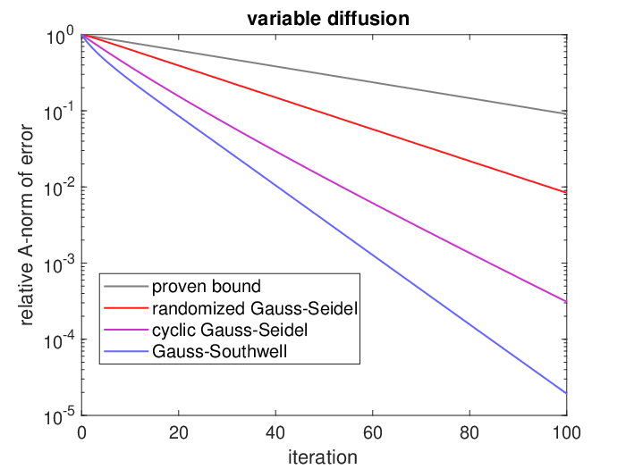
The top row of Figure 1 gives results for the constant diffusion case (17). The left diagram shows the relative -norm of the errors for randomized Gauss-Seidel with uniform probabilities , standard (“cyclic”) Gauss-Seidel and Gauss-Southwell with the greedy pick rule (3). For randomized Gauss-Seidel we actually give here—as in all other experiments—the averages for ten runs which we regard as an approximation to the expected values. The plot to the right shows that the convergence behavior of these ten different runs exhibit only mild deviations. The plot on the left also contains the bound of Theorem 2. We see that randomized Gauss-Seidel converges approximately half as fast as cyclic Gauss-Seidel, that Gauss-Southwell converges somewhat faster than cyclic Gauss-Seidel, and that the thoretical bounds are not very tight.
The bottom row of Figure 1 shows results for variable diffusion according to (18). Convergence is slower than in the constant diffusion case. The left plot has the results for the “optimial” probabilities and the “optimal” greedy-pick (12), for which the bounds of Theorem 2 hold again and are also reported, whereas the right plot shows the results for the uniform probabilities and the greedy-pick rule (3). In this case, the bound of Theorem 2 holds with , and this bound is also plotted. Interestingly, the two plots are virtually indistinguishable, except for a tiny improvement of randomized Gauss-Seidel when using “optimal” probabilities. We conclude that the choice of probabilities or the greedy pick rule has only a very marginal effect in this example. The plots also show that the proven bounds can be pessimistic in the sense that the actual convergence is significantly faster. This is not uncommon when dealing with randomized algorithms, and we will address this further when discussing the numerical results illustrating the new convergence theorems for diagonally dominant matrices in Section 3.
Although not being further addressed in this paper, we now shortly present basic numerical results on the performance of the various relaxation methods when used as a smoother in a multigrid method. This was mentioned as a possible application in the introduction. We consider a V-cycle multigrid method for the standard discrete Laplacian on a grid (with a power of 2) with Dirichlet boundary conditions. Restriction and prolongation are done via the usual linear interpolation, doubling the grid spacing from one level to the next and going down to a minimum grid size of ; see Trottenberg et al. 2000. For each smoother, on each level with a grid size of we perform a constant number of post- and pre-smoothing “iterations” amounting to relaxations. For standard Gauss-Seidel and Gauss-Southwell we use , whereas for randomized Gauss-Seidel we tested and .


Figure 2 indicates that randomized Gauss-Seidel has its potential for being used as a smoother in multigrid, provided that its slower convergence can be outweighed by a more efficient implementation, as it might be possible in a parallel environment. The left plot gives convergence plots for . The right plot reports the number of V-cycles required to reduce the initial residual by a factor of for various grid sizes . We see that the convergence speed with randomized Gauss-Seidel and Gauss-Southwell smoothing is independent of the grid size just as with standard Gauss-Seidel smoothing, thus preserving one of the most important properties of the multigrid approach. An interesting feature that random Gauss-Seidel shares with the Gauss-Southwell method is that we can prescribe a fractional number of smoothing iterations and thus adapt the computational work on a finer scale than with standard Gauss-Seidel. The figure also shows that for this example Gauss-Southwell yields faster convergence than standard Gauss-Seidel for the same number of relaxations.
3 Results for non-Hermitian matrices
We now present several theorems which are counterparts to Theorem 2 for classes of not necessarily Hermitian matrices, and the iteration matrix in (2) may arise from a general splitting other than the (relaxed) Jacobi splitting. In place of the -norm we will now use weighted -norms.
Definition 3.
For a given vector with positive components , , the weighted -norm on is defined as
Clearly, the standard -norm is obtained for . It is easy to see that the associated operator norm for is the weighted column sum-norm
In the theorems to follow we will state results in terms of the preconditioned residual
and we denote the preconditioned matrix .
Our first theorem assumes and gives bounds on the weighted -norms of the preconditioned residuals in Algorithms 2 and 3 similar in nature to those in Theorem 2.
Theorem 4.
Consider the weighted column sums
and assume that . Set .
- (i)
- (ii)
Proof.
If is the index chosen at iteration , we have
which gives
We therefore have
| (24) | |||||
To prove part (i) we use (24) to see that the expected value of the norm of the residual , conditioned to the given value for satisfies
from which we get (20). Moreover, the minimum is not larger than the convex combination , and this value is attained for if we choose .
The convergence results of Theorem 4 are given in terms of the weighted -norm, since it is this norm for which we can prove a decrease in every relaxation due to the assumption . As we will soon see, for randomized Gauss-Seidel and Gauss-Southwell this assumption is equivalent to a (generalized) diagonal dominance assumption on , a condition which is often fulfilled in applications and which can be checked easily, at least when the weights are all 1. In this context, it is worth mentioning that results like the bound (22) yield a bound on the convergence factor of the sequence , the standard measure of the convergence rate for a linearly zero-convergent sequence defined as
see, e.g., Ortega and Rheinboldt 2000. The -factor is independent of the norm , and results like (22) may be interpreted in a norm-independent manner by saying that
From Theorem 4 we see that with the optimal choices for the probabilities or the weights , the proven bounds for randomized relaxation and greedy relaxation are identical. So from the point of view of the established theory we cannot conclude that randomized would outperform greedy or vice-versa. In all our practical experiments, though, the greedy approach exposed faster convergence than the randomized approach.
Also note that if we just take for all in randomized relaxation, then
and the same value is attained for in greedy relaxation if we take for all . The optimal value is attained for the greedy pick rule (23). If we take the standard greedy pick rule (3), i.e. for all , we have
which, depending on the values of can be smaller or larger than but is certainly never larger than obtained with the pick rule (23).
In Theorem 4 we need to know the weights and with them the weighted column sums in order to be able to choose the probabilities or the greedy pick for which we get the strongest convergence bound, i.e., the largest value for and . For example, it might be that we can take , such that reduces to the standard -norm. However, it might also be that we know that for some without knowing explicitly. Theorem 4 tells us that we still have convergence for any choice of probabilities in randomized relaxation or weights in greedy relaxation, but the proven convergence bounds are weaker than for the “optimal” probabilites (21) or weights (23).
In light of this discussion it is interesting that for a particular vector of weights we can somehow reverse the situation, at least for the randomized iteration: We know how to choose the corresponding optimal values for the probabilities while we do not need to know explicitly.
In order to prepare this result we recall the following left eigenvector version of the Perron-Frobenius theorem; see, e.g., Varga 1962. Note that a square matrix is called irreducible if there is no permutation matrix such that has a block structure with a zero off-diagonal block. We also use the notation (“ is nonnegative”) if all entries of are nonnegative. Similarly, a vector is called nonnegative () or positive (), if all its components are nonnegative or positive, respectively.
Theorem 5.
Let , , be irreducible. Then there exists a positive vector , the “left Perron vector” of , such that , where is the spectral radius of . Moreover, is unique up to scaling with a positive scalar.
If is not irreducible, a positive left Perron vector needs not necessarily exist. However, we have the following approximation result which we state as a lemma for future reference.
Lemma 6.
Assume that is nonnegative. Then, for any there exists a positive vector such that .
Proof.
For given , due to the continuity of the spectral radius we can choose small enough such that the spectral radius of the irreducible matrix , the matrix of all ones, is less or equal than . Now take as the left Perron vector of . ∎
We are now ready to prove the following theorem where we use the notation for the matrix resulting from when replacing each entry by its absolute value. Interestingly, the theorem establishes a situation where we know how to choose optimal probabilities (in the sense of the proven bounds) without explicit knowledge of the weights.
Theorem 7.
Assume that and consider randomized relaxation (Algorithm 3).
- (i)
If is irreducible, then there exists a positive vector of weights such that the weighted -norm of the preconditioned residuals of the iterates satisfies
Moreover, is maximized if one takes for ; its value then is .
- (ii)
If is not irreducible, then for every such that there exists a positive vector of weights such that the weighted -norm of the preconditioned residuals of the iterates satisfies
Moreover, is maximized if one takes for ; its value then is .
Proof.
4 Randomized Gauss-Seidel and Gauss-Southwell for H-matrices
Building on Theorem 4 we now derive convergence results for the randomized Gauss-Seidel and the Gauss-Southwell method when is an H-matrix.
Definition 8.
(See, e.g., Berman and Plemmons 1994)
- (i)
A matrix is called an M-matrix if for and it is non-singular with .
- (ii)
A matrix is called an H-matrix, if its comparison matrix with
is an M-matrix.
Clearly, an M-matrix is also an H-matrix. For our purposes it is important that H-matrices can equivalently be characterized as being generalized diagonally dominant.
Lemma 9.
Let be an H-matrix. Then
- (i)
There exists a positive vector such that is generalized diagonally dominant by rows, i.e.,
- (ii)
There exists a positive vector such that is generalized diagonally dominant by columns, i.e.
Proof.
Part (i) can be found in many text books, one can take , with . Part (ii) follows similarly by taking as the row vector . ∎
The lemma implies the following immediate corollary.
Corollary 10.
Let be an H-matrix and let be its Jacobi splitting with the diagonal part of . Then the iteration matrix belonging to the Jacobi splitting of satisfies with the vector from Lemma 9(ii).
With these preparations we easily obtain the following first theorem on the (unrelaxed) randomized Gauss-Seidel and Gauss-Southwell methods. We formulate it using the residuals of the original equation.
Theorem 11.
Let be an H-matrix and let be a positive vector such that . Let be the Jacobi splitting of and put . Moreover, let with . Then
- (i)
All weighted column sums
(25) are less than 1.
- (ii)
In the randomized Gauss-Seidel method, i.e. Algorithm 3 for , the expected values of the -weighted -norm of the original residuals satisfy
where and for . The value of is maximized for the choice , and the resulting value for is .
- (iii)
Proof.
For (i) observe that we have for and thus, since for and ,
Parts (ii) and (iii) now follow directly from Theorem 4, observing that for the residual we have . ∎
Note that for Gauss-Southwell the greedy pick rule (5) with weights based on the preconditioned residual is equivalent to the greedy pick rule (4) based on the original residual with weights .
Instead of changing the weights from to , it is also possible to obtain a bound for the -weighted -norm, where, in addition, the same optimal choice for the in the randomized Gauss-Seidel iteration yields the same as that of Theorem 11, and similarly for the Gauss-Southwell iteration.
Theorem 12.
Let be an H-matrix and let be a positive vector such that . Then
- (i)
In the randomized Gauss-Seidel method the expected values of the -weighted -norm of the residuals satisfy
where and , from (25), for . The value of is maximized for the choice
(26) and the resulting value for is .
- (ii)
Proof.
If is the index chosen in iteration in randomized Gauss-Seidel or Gauss-Southwell, we have from (8)
This gives
This is exactly the same relation as (24), but now for the original residuals rather than the preconditioned ones. Parts (i) and (ii) therefore follow exactly in the same manner as in the proof of Theorem 4. ∎
Let us mention that, if and thus is irreducible, the left Perron vector of is a vector with . As was discussed after Theorem 4 this means that with respect to the weigths from this vector we know the optimal probabilities in randomized Gauss-Seidel to be , i.e., we do not need to know explicitly. According to Lemma 6, a similar observation holds in an approximate sense with arbitrary precision when is not irreducible.
We also remark that the preconditioned residual satisfies with from Theorems 11 and 12. So with these two theorems we have obtained identical convergence bounds for the -weighted -norm of the unpreconditioned and the preconditioned residuals.
Theorem 11 can be extended to relaxed randomized Gauss-Seidel iterations. We formulate the results only for the case where the weight vector is the left Perron vector. While this is not mandatory as long as the relaxation parameter satisfies , it is crucial for the part which extends the range of to values larger than 1.
Theorem 13.
Let be an H-matrix and let be its Jacobi splitting. Put and . Assume that and define . Consider the relaxed randomized Gauss-Seidel iteration, i.e., Algorithm 3 with the matrix from (7). Then
- (i)
If and thus is irreducible, then with the left Perron vector of and the positive vector with components , the expected values for the -weighted -norm of the residuals satisfy
where , . The value of is maximized for the choice , and the resulting value for is .
- (ii)
If is not irreducible, then for every such that there exists a positive vector such that the expected values for the weighted -norm of the residuals satisfy
where , . The value of is maximized for the choice , and the resulting value for is .
Proof.
We indeed have since by Corollary 10 the operator norm is less than 1 for some vector . Assume first that is irreducible and let be the left Perron vector of . Then we have for all
which for the weighted column sums of the matrix belonging to the relaxed iteration gives
Since we have that for . The result now follows applying Theorem 4 with the weight vector , using the facts that all weighted column sums are now equal to and that , which gives the weights in (i).
If is not irreducible, the proof proceeds in exactly the same manner, chosing as a vector for which ; see the discussion after Theorem 5. ∎
For the same reasons as those explained after Theorem 7, it is not possible to expand Theorem 13 to Gauss-Southwell unless we we know the Perron vector and include it into the greedy pick rule. We do not state this as a separate theorem.
Numerical example
We consider again the implicit Euler rule for the convection-diffusion equation (15), now with a non-vanishing and non-constant velocity field describing a re-circulating flow,
We will consider the two choice (weak convection) and (strong convection); the diffusion coefficients and are constant and equal to 1. With and , as in the example in section 2, the matrix from (16) is diagonally dominant for both and . So we take the weight vector to have all components equal to 1 and we report results on the -norm of the residuals for randomized Gauss-Seidel and Gauss-Southwell as an illustration of Theorem 12. Since this time we are interested in the residuals rather than in the errors, it is not mandatory to fix the right hand side such that we know the solution, but to stay in line with the earlier experiments we actually did so with the solution being again the discretization of .
The top row of Figure 3 displays, as before, these -norms only after every relaxations, considered as one iteration. For both values of we take the probabilities from (26) in randomized Gauss-Seidel and the greedy pick rule (27) for Gauss-Southwell, so that Theorem 12 applies, and the plots also report the bounds for the 1-norm of the residual given in that theorem.


The plots in the top row show a similar behavior of the different relaxation methods as in the hpd case, with Gauss-Southwell being fastest, especially for strong convection, and randomized Gauss-Seidel converging roughly half as fast as cyclic Gauss-Seidel—and this for both values of . As opposed to the hpd case, the theoretical bounds are now much closer to the actually observed convergence behavior of the randomized relaxations. For the bounds are actually that close that in the graph they are hidden behind the reported residual norms. For the bounds can be distinguished from the residual norms in the plots, but they are still remarkably close.
The bottom row of Figure 3 contains results for the cyclic and the randomized Kaczmarz methods. With denoting the th row of , and the corresponding column vector, relaxing component in Kaczmarz amounts to the update
We report these results since they allow for a comparison, randomized Kaczmarz being one of the most prominent randomized system solvers for non-symmetric systems.
The plots report the 2-norm of the error for which we know a bound given by the right hand side in the inequality
where is the smallest non-zero singular value of . This bound holds if ’optimal’ probabilities are chosen, see Strohmer and Vershynin 2009, as , which is what we did for these experiments.
We see that as with Gauss-Seidel, the cyclic algorithms converges approximately twice as fast than the randomized algorithm. The theoretical bounds are less sharp than for the Gauss-Seidel methods. For both matrices, the cyclic and randomized Kaczmarz methods converge significantly slower than their Gauss-Seidel counterparts while, moreover, one relaxation in Kaczmarz needs approximately twice as many operations than in Gauss-Seidel. Since the plots on the top row report -norms rather than 2-norms of the error, let us just mention that in the weak convection case, , the relative 2-norm of the residual in the randomized Gauss-Seidel run from the top row of Figure 3 is at iteration 41, and in the strong convection case, , it is at iteration 60. On the other hand, randomized Kaczmarz failed to converge to the desired tolerance of within 100 iterations.
5 Conclusion
We developed theoretical convergence bounds for both randomized and greedy pick relaxations for nonsingular linear systems. While we mainly reviewed results for the Gauss-Seidel relaxations in the case of a Hermitian positive definite matrix , we presented several new convergence results for nonsymmetric matrices in the case where the iteration matrix has a weighted -norm less than 1. From this we could deduce several convergence results for randomized Gauss-Seidel and Gauss-Southwell relaxations for H-matrices. We also presented results which show how to choose the probability distributions (in case of randomized relaxations) or the greedy pick rule (in case of greedy iterations) which minimize our convergence bounds. Numerical experiments illustrate our theoretical results and also show that the methods analyzed are faster than Kaczmarz for square matrices.
Acknowledgement.
We want to thank Karsten Kahl from University of Wuppertal for sharing his Matlab implementations constructing convection-diffusion matrices with us. We also thank Vahid Mahzoon from Temple University for some preliminary experiments which helped guide our thinking. We express our gratitude to the two reviewers for their comments and questions, which helped improve our presentation.
References
- Avron et al. [2015] Haim Avron, Alex Druinsky, and Anshul Gupta. Revisiting asynchronous linear solvers: Provable convergence rate through randomization. Journal of the ACM, 62, 2015. Article 51 (27 pages).
- Bai and Wu [2018a] Zhong-Zhi Bai and Wen-Ting Wu. On convergence rate of the randomized Kaczmarz method. Linear Algebra and its Applications, 553:252–269, 2018a.
- Bai and Wu [2018b] Zhong-Zhi Bai and Wen-Ting Wu. On relaxed greedy randomized Kaczmarz methods for solving large sparse linear systems. Applied Mathematics Letters, 83:21–26, 2018b.
- Bai and Wu [2021] Zhong-Zhi Bai and Wen-Ting Wu. On greedy randomized augmented Kaczmarz method for solving large sparse inconsistent linear systems. SIAM Journal on Scientific Computing, 43:A3892–A3911, 2021.
- Bai et al. [2021] Zhong-Zhi Bai, Lu Wang, and Wen-Ting Wu. On convergence rate of the randomized Gauss-Seidel method. Linear Algebra and its Applications, 611:237–252, 2021.
- Bai et al. [2022] Zhong-Zhi Bai, Lu Wang, and Galina V. Muratova. On relaxed greedy randomized augmented Kaczmarz methods for solving large sparse inconsistent linear systems. East Asian Journal on Applied Mathematics, 12:323–332, 2022.
- Berman and Plemmons [1994] Abraham Berman and Robert J. Plemmons. Nonnegative Matrices in the Mathematical Sciences, volume 9 of Classics in Applied Mathematics. SIAM, Philadelphia, 1994.
- Du [2019] Kui Du. Tight upper bounds for the convergence of the randomized extended Kaczmarz and Gauss-Seidel algorithms. Numerical Linear Algebra with Applications, 26:e2233, 2019. 14 pages.
- Frommer and Szyld [2000] Andreas Frommer and Daniel B. Szyld. On asynchronous iterations. Journal of Computational and Applied Mathematics, 123:201–216, 2000.
- Glusa et al. [2020] Christian Glusa, Erik G. Boman, Edmond Chow, Sivasankaran Rajamanickam, and Daniel B. Szyld. Scalable asynchronous domain decomposition solvers. SIAM Journal on Scientific Computing, 42:C384–C409, 2020.
- Gower and Richtárk [2015] Robert M. Gower and Peter Richtárk. Randomized iterative methods for linear systems. SIAM Journal on Matrix Analysis and Applications, 36:1660–1690, 2015.
- Gower et al. [2021] Robert M. Gower, Denali Molitor, Jacob Moorman, and Deanna Needell. On adaptive sketch-and-project for solving linear systems. SIAM Journal on Matrix Analysis and Applications, 42:954–989, 2021.
- Griebel and Oswald [2012] Michael Griebel and Peter Oswald. Greedy and radomized versions of the multiplicative Schwarz method. Linear Algebra and its Applications, 437:1596–1610, 2012.
- Guan et al. [2020] Ying-Jun Guan, Wei-Guo Li, Li-Li Xing, and Tian-Tian Qiao. A note on convergence rate of randomized Kaczmarz method. Calcolo, 57:Paper No. 26, 11, 2020.
- Guo and Li [2018] Jun Han Guo and Wei Guo Li. The randomized Kaczmarz method with a new random selection rule. Numerical Mathematics. A Journal of Chinese Universities. Gaodeng Xuexiao Jisuan Shuxue Xuebao, 40:65–75, 2018.
- Haddock and Ma [2021] Jamie Haddock and Anna Ma. Greed works: An improved analysis of sampling Kaczmarz-Motzkin. SIAM Journal on Mathematics of Data Science, 3:342–368, 2021.
- Kaczmarz [1937] Stefan Kaczmarz. Angenäherte Auflösung von Systemen linearer Gleichungen. Bulletin International de l’Academie Polonaise de Sciences et de Lettres, Cl. Sci. Math. Nat. A, 35:355–357, 1937.
- Kannan and Vempala [2017] Ravindran Kannan and Santosh Vempala. Randomized algorithms in numerical linear algebra. Acta Numerica, pages 95–135, 2017.
- Leventhal and Lewis [2010] Dennis Leventhal and Adrian S. Lewis. Randomized methods for linear constraints: Convergence rates and conditioning. Mathematics of Operations Research, 35:641–654, 2010.
- Ma et al. [2015] Anna Ma, Deanna Needell, and Aaditya Ramdas. Convergence properties of the randomized randomized extended Gauss-Seidel and Kaczmarz algorithms. SIAM Journal on Matrix Analysis and Applications, 36:1590–1604, 2015.
- Magoulès et al. [2017] Frédéric Magoulès, Daniel B. Szyld, and Cédric Venet. Asynchronous optimized Schwarz methods with and without overlap. Numerische Mathematik, 137:199–227, 2017.
- Martinsson and Tropp [2020] Per-Gunnar Martinsson and Joel A. Tropp. Randomized numerical linear algebra: foundations and algorithms. Acta Numerica, pages 403–572, 2020.
- Ortega and Rheinboldt [2000] J. M. Ortega and W. C. Rheinboldt. Iterative Solution of Nonlinear Equations in Several Variables, volume 30 of Classics in Applied Mathematics. Society for Industrial and Applied Mathematics (SIAM), Philadelphia, PA, 2000. Reprint of the 1970 original.
- Richtárik and Takáč [2020] Peter Richtárik and Martin Takáč. Stochastic reformulations of linear systems: Algorithms and convergence theory. SIAM Journal on Matrix Analysis and Applications, 41:487–524, 2020.
- Rüde [1993] Ulrich Rüde. Mathematical and Computational Techniques for Multigrid Adaptive Methods. SIAM, Philadelphia, 1993.
- Saad [1996] Yousef Saad. Iterative Methods for Sparse Linear Systems. PWS Publishing Co., Boston, 1996. Second edition, SIAM, Philadelphia, 2003.
- Saad [2020] Yousef Saad. Iterative methods for linear systems of equations: A brief historical journey. In Susanne C. Brenner, Igor Shparlinski, Chi-Wang Shu, and Daniel B. Szyld, editors, Mathematics of Computation 75 Years. American Mathematical Society, Providence, RI, 2020.
- Smith et al. [1996] Barry F. Smith, Petter E. Bjørstad, and William Gropp. Domain Decomposition: Parallel Multilevel Methods for Elliptic Partial Differential Equations. Cambridge University Press, 1996.
- Steinerberger [2021a] Stefan Steinerberger. A weighted randomized Kaczmarz method for solving linear systems. Mathematics of Computation, 90:2815–2826, 2021a.
- Steinerberger [2021b] Stefan Steinerberger. Randomized Kaczmarz converges along small singular vectors. SIAM Journal on Matrix Analysis and Applications, 42:608–615, 2021b.
- Strikwerda [2002] John C. Strikwerda. A probabilistic analysis of asynchronous iteration. Linear Algebra and its Applications, 349:125–154, 2002.
- Strohmer and Vershynin [2009] Thomas Strohmer and Roman Vershynin. A randomized Kaczmarz algorithm with exponential convergence. J. Fourier Anal. Appl., 15(2):262–278, 2009. 10.1007/s00041-008-9030-4.
- Trottenberg et al. [2000] Ulrich Trottenberg, Cornelius Oosterlee, and Anton Schuller. Multigrid. Academic Press, New York, 2000.
- Varga [1962] Richard S. Varga. Matrix Iterative Analysis. Prentice-Hall, Englewood Cliffs, New Jersey, 1962. Second Edition, revised and expanded, Springer, Berlin, 2000.
- Wang et al. [2022] Fang Wang, Weiguo Li, Wendi Bao, and Li Liu. Greedy randomized and maximal wwighted residual Kaczmarz methods with oblique projection. Electronic Research Archive, 30:1158–1186, 2022.
- Wolfson-Pou and Chow [2017] Jordi Wolfson-Pou and Edmond Chow. Distributed Southwell: An iterative method with low communication costs. In International Conference for High Performance Computing, Networking, Storage, and Analysis (SC17), Denver, CO. Association for Computing Machinery, 2017. (13 pages).
- Yang [2021] Xi Yang. A geometric probability randomized Kaczmarz method for large scale linear systems. Applied Numerical Mathematics, 164:139–160, 2021.