Towards explainable evaluation of language models on the semantic similarity of visual concepts

Considering $\mathcal{V}$ as a set of visual concepts, concept agreement measures the percentage of ground truth concepts $\mathcal{V}(I_{g})$ contained in the retrieved concept set $\mathcal{V}(I_{r})$ over all $\mathcal{V}(I_{g})$ concepts for each $f_{i}$. Let $V_{(g,r)}=\mathcal{V}(I_{g})\>\cap\>\mathcal{V}(I_{r})$ the set of common concepts:

$CA_{f}=\frac{|V_{(g,r)}|}{|\mathcal{V}(I_{g})|}$, $f=(I_{g},I_{r})$

Higher CA indicates higher concept similarity. For example, if $\mathcal{V}(I_{r})=\{\mathsf{Dog,Frisbee,Park}\}$ and $\mathcal{V}(I_{g})=\{\mathsf{Dog,Ball,Park}\}$, then the CA=$\frac{2}{3}$. On the other hand, if $\mathcal{V}^{\prime}(I_{r})=\{\mathsf{Cat,Fish}\}$, then CA=0, as no overlap exists. This way we can confidently conclude that the first retrieved image is conceptually closer to the ground truth than the second, and by extension the model used to retrieve the first image is better with respect to CA.

aims to provide a distance measure between concepts present exclusively in either $\mathcal{V}(I_{g})$ or $\mathcal{V}(I_{r})$. For example, we would expect the set $\{\mathsf{Dog,Frisbee,Park}\}$ to be more similar to $\{\mathsf{Dog,Ball,Park}\}$ than $\{\mathsf{Dog,Cat,Park}\}$, since the non-common concept $\mathsf{Frisbee}$ is conceptually closer to $\mathsf{Ball}$ than $\mathsf{Cat}$. Mathematically, let $D_{g}=V_{(g,r)}-\mathcal{V}(I_{r})$ and $D_{r}=V_{(g,r)}-\mathcal{V}(I_{g})$, with both $D_{g},D_{r}\neq\emptyset$. Other than that, $D_{g}$ and $D_{r}$ may contain different number of concepts. Then, a measure of concept distance can be provided by calculating the path similarity score $ps$ of corresponding WordNet Fellbaum 1998 synset pairs, based on the shortest available path between those two concepts. Path similarity $ps$ ranges between 0 and 1.

An optimistic NCS metric returns the maximum possible cumulative $ps$ averaged over the number of pairs, by appropriately selecting concept pairs between non-empty $D_{g}$ and $D_{r}$. The maximization of NCS requires a dynamic programming solution, as naive strategies taking into account all possible $D_{g}$ and $D_{r}$ pairs would yield a factorial amount of combinations. To trespass this prohibitive complexity, we create a bipartite graph $G=(D_{g},D_{r},E)$ from $D_{g}$ and $D_{r}$: all concept nodes from the one set are matched with all the nodes of the other via edges $e_{y}\in E,y=1,2,...,|D_{g}|\times|D_{r}|$, while no edges are allowed within the same set. Edge weights $w_{e_{y}}$ correspond to WordNet $ps$ scores between synsets of connected nodes.

Consequently, the maximum weight bipartite matching on $G$ refers to pairing $D_{g}$ and $D_{r}$ concepts so that the cumulative edge weight is maximized. An optimized version of the Hungarian algorithm Kuhn 1955; Galil 1986 implemented by NetworkX¹¹ 1 NetworkX max weight matching reduces the computational complexity of finding the maximum $ps$ to $O(|V|^{3})$, where $|V|=max(|D_{g}|,|D_{r}|)$.

Therefore, NCS can be written as:

$NCS_{f}=avg(max\_weight\_match(G))$, $G=(V_{(g,r)}-\mathcal{V}(I_{r}),V_{(g,r)}-\mathcal{V}(I_{g}),E))$

Higher NCS scores reveal more similar concepts.

Real world scenes may contain repeated instances of same-class concepts, forming concept multisets $\mathcal{V}_{m}=\{(\mathcal{V}_{1},|\mathcal{V}_{1}|),(\mathcal{V}_{2},|\mathcal{V}_{2}|),...,(\mathcal{V}_{x},|\mathcal{V}_{x}|)\}$, where $\mathcal{V}_{1},\mathcal{V}_{2},...,\mathcal{V}_{x}$ denote concept categories, and $|\mathcal{V}_{1}|,|\mathcal{V}_{2}|,...,|\mathcal{V}_{x}|$ cardinalities per category. The cardinality per concept category is called concept multiplicity in the multiset. CE penalizes differences in multiplicities between common concepts of $I_{g}$ and $I_{r}$ for each $f_{i}$:

Higher CE scores demonstrate higher enumeration disagreement, deeming lower CE values more favorable. For example, if $I_{g}$ contained 10 dogs and 1 frisbee $\{(\mathsf{Dog},10),(\mathsf{Frisbee},1)\}$, a retrieved $I_{r}$ with 1 dog and 1 frisbee would have CE=9, while an $I^{\prime}_{r}$ with 10 dogs and 1 ball would have a CE=0. Therefore, the first image yields a worse CE score than the second, even though the second would have worse CA and NCS scores than the first one.

Even in cases where there is a high agreement of objects and multiplicities between $I_{g}$ and $I_{r}$, disagreement in object sizes may correspond to semantically divergent scenes. For example an image with a dog in the foreground (large bounding box) is different than an image of a dog in the background (small bounding box). To capture this difference, we design an optimistic SD metric which returns the area differences of bounding boxes $\mathcal{D}_{A}=|A_{g}-A_{r}|$ for all available object matchings. Such matchings occur by pairing concepts of the same category $u$ between $\mathcal{I}_{g}$ and $\mathcal{I}_{r}$ up to the point that no more unique pairs can be constructed. This is equivalent of creating bipartite graph $G_{u}=(\mathcal{V}_{u}(I_{g}),\mathcal{V}_{u}(I_{r}),E)$, where $\mathcal{V}_{u}(I_{g}),\mathcal{V}_{u}(I_{r})$ belong in the same $u$ and edge weights $w_{e_{y}},e_{y}\in E,y=1,2,...,|\mathcal{V}(I_{g})|\times|\mathcal{V}(I_{r})|$ denote the area difference $\mathcal{D}_{A}$ between concept nodes. Pairing concepts with similar bounding box areas can be considered as the optimal choice, therefore node pairs connected by lower edge weights $w_{e_{y}}$ are preferred. Finding the minimum weight matching provides the most similar pairs size-wise, and can be solved in polynomial time using the NetworkX²² 2 NetworkX min weight full matching implementation of Karp algorithm Karp 1978. The matching process is repeated for all concept categories in the multiset $\mathcal{V}_{m}$, resulting in a set of graphs $G_{m}$:

A simplified binary version of SD increases a sum if area differences of paired concepts are above a predefined threshold $T_{D}$.

are extracted via relevant WordNet functions for any adjective present in a query. If more than one antonyms are returned, one is randomly picked to substitute the actual word.

refers to changing colors present in the sentence with another distant color. Color distance is provided via the RGB values of Matplotlib colors³³ 3 Matplotlib colors. We set a proximity threshold to ensure perceptually non-negligible color changes. Two possible substitutions are attempted: either considering all RGB colors (color-all), or colors only mentioned in the dataset (color-in).

is an antonym substitution specialized in sizes. Words such as large, big, enormous, huge are substituted with a random choice among small, little, minor, tiny and vice versa.

The real power of our proposed metrics lies in local level. We present an example from the color and details failure category below. Given a query $q_{i}$ (caption), Figure 4 shows the ground truth $I_{g_{i}}$ (left) and the retrieved $I_{r_{i}}$ (right).

The set of ground truth object synsets is {$\mathsf{trunk.n.01}$, $\mathsf{hill.n.01}$, $\mathsf{tree.n.01}$, $\mathsf{sky.n.01}$, $\mathsf{field.n.01}$, $\mathsf{branch.n.01}$, $\mathsf{head.n.01}$, $\mathsf{leg.n.01}$, $\mathsf{leaf.n.01}$, $\mathsf{zebra.n.01}$, $\mathsf{mane.n.01}$} of cardinality 11, and the set of retrieved ones is {$\mathsf{grassland.n.01}$, $\mathsf{field.n.01}$, $\mathsf{zebra.n.01}$, $\mathsf{mane.n.01}$, $\mathsf{grass.n.01}$} of cardinality 5. Common synsets are {$\mathsf{zebra.n.01}$, $\mathsf{mane.n.01}$, $\mathsf{field.n.01}$} of cardinality=3, resulting in CA_i=27.28%. Regarding NCS, the constructed bipartite graph $G$ contains $|V|$=10, $|E|$=16, and the best matched synset pairs according to the maximum weight matching are {$\mathsf{hill.n.01}$, $\mathsf{grassland.n.01}$} with $ps$=0.111, and {$\mathsf{tree.n.01}$, $\mathsf{grass.n.01}$} with $ps$=0.167. The average $ps$ for all matched pairs leads to NCS_i=0.139. Common object enumeration provides the following multisets: $\mathcal{V}^{g}_{m}$ = {$\mathsf{zebra.n.01}$, 5, $\mathsf{field.n.01}$, 1, $\mathsf{mane.n.01}$, 1} and $\mathcal{V}^{r}_{m}$ ={$\mathsf{zebra.n.01}$, 7, $\mathsf{field.n.01}$, 1, $\mathsf{mane.n.01}$, 5}. Therefore, CE_i= 6. As for SD for $T_{D}$=1, 3 bipartite graphs are created for the 3 common synsets. The first graph $G_{mane}$ contains $|V|$=6 and $|E|$=5, resulting in 1 minimum weight matching of weight $D_{A}$=2.30$\geq T_{D}$. Therefore SD_mane=1=SD_i. The second graph $G_{zebra}$ consists of $|V|$=11 and $|E|$=28, resulting in 4 minimum weight matchings, from which none trespassed the threshold $T_{D}$, resulting in SD_zebra=0, thus maintaining SD_i=1. Finally, the $G_{field}$ graph of $|V|$=2 and $|E|$=1, leads to 1 minimum weight matching of weight $D_{A}$=1.369$\geq T_{D}$, resulting in SD_field=1, which increases the total sum SD_i=2. Having in total 6 matches for all three graphs, the averaged SD_i=33.3% for this $f_{i}$.

Perceptually, a major $I_{g_{i}},I_{r_{i}}$ disagreement can be attributed to not satisfying lush, green attributes rather than semantics addressed by our metrics. Indeed, human evaluators rated $I_{r_{i}}$-$q_{i}$ relevance with 6/10 on average and all of them marked details and color as the failure categories. As for traditional ranking metrics, $I_{g_{i}}$ was placed in $\mathsf{rank}_{g_{i}}$=294 with reciprocal rank score of 0.0034 and R@k=0, k=1,5,10. Obviously, we cannot extract much information in local level about how much $I_{g_{i}}$ and $I_{r_{i}}$ conceptually deviate and what we should potentially regard and request from retrieved instances (colors such as green instead of yellow, details such as lush instead of arid) to ascend in the rank. To this end, we conclude that traditional ranking metrics are only helpful in a very abstract level.

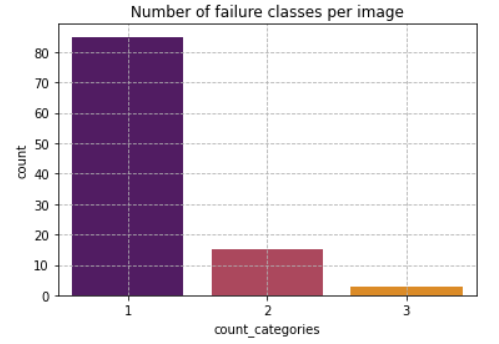
Results regarding misperceived semantics classes are presented in Table 2. The 82.52% of evaluated image pairs resulted in one semantic class disagreement, while the remaining 14.56% and 2.91% contained two and three semantic class disagreements respectively. The average rating over all classes was 8.47/10.

First, human evaluation experiments can indicate the degree of strictness of our automated metrics, as any query-agnostic metric may over-penalize semantics present in the $I_{g_{i}}$ and $c_{i}$ but not in $q_{i}$. Indeed, query-informed variants of our metrics are more relaxed. Moreover, patterns in reported failures also indicate patterns imprinted in the learned linguistic representations. Traditional ranking metrics cannot derive such fine-grained observations.

The frequent class of successful alternatives indicates that even when automatic metrics consider an $I_{r_{i}}$ as failure, it may actually be a conceptually correct answer to $q_{i}$. Qualitative analysis over successful alternatives further demonstrated that almost all $(I_{g_{i}},I_{r_{i}})$ pairs of this class were visually divergent, even though conceptually equivalent. Also, details and object color failure classes appeared often enough, indicating that those semantics are rather bypassed in order for others to be preserved. Combinations of semantics did not present any significant pattern; all semantics co-occurrences appeared in less than 10% of the evaluated instances. However, we did observe some frequent rules, which can be translated as: if semantic A disagrees, then semantic B will disagree as well. The rule action$\rightarrow$details (if action appears then details will appear) is observed in 54.37% of the instances containing action; object enumeration $\rightarrow$object color covers 17.48% of the instances containing color; finally, the reverse rule object color$\rightarrow$object enumeration was observed in 11.65% of the instances containing enumeration.

We present global query-agnostic results for our metrics. Despite our metrics being more meaningful in local level, global evaluation is useful for model benchmarking.

With 134630 common concepts between all $(I_{g},I_{r})_{i}\in\mathcal{F}$, the average concept agreement (CA) value is 22.29%, meaning that on average almost the 1/4th of $I_{g}$ concepts appear in $I_{r}$.

With 903987 non-common concepts between all $(I_{g},I_{r})$, and 134630 common ones, we retrieve 627833 and 110839 WordNet synsets respectively. The maximum weight matching between non-common synsets results in 184747 maximum weight matchings, equivalent to the 29.43% of all non-common synsets. Averaging over matchings (WordNet path similarities) for all $(I_{g},I_{r})$, provides the average non-common concept similarity (NCS) score of 0.122.

With 41244 concept sets of same multiplicity and 69595 of different multiplicities regarding matched concept categories for all $(I_{g},I_{r})$, most common concept enumeration (CE)=1 and average CE=8.638 instances for concepts of the same category reveals that in most cases there are not major enumeration differences.

Focusing on the binary SD, we set the area difference threshold $T_{D}$=100%, increasing size disagreement (SD) by 1 iff $\mathcal{D}_{A}\geq 1$ between two concept bounding box areas. Thus, average SD=20.35% for all $(I_{g},I_{r})$, indicating that around 1/5th of common objects have non-negligible size differences.

Our metrics in global level reveal some extra capabilities. Most lower-ranked instances contained erroneous annotations, allowing a post-hoc dataset cleaning step that could not have been automatically realized otherwise.

Global results regarding our proposed metrics for all the models are presented in Table 3. Moreover, we offer some additional insights:

• •

  Object hit: total number of common objects found between ground truth - wrongly retrieved images ($I_{g},I_{r}$) at top-1 position.

• •

  Object miss: total number of ground truth objects not found in top-1 retrieved images.

• •

  Matched % synsets: Percentage of ground truth synsets found in top-1 retrieved images out of all ground truth synsets.

• •

  Average % object enumeration disagreement: percentage of objects having the wrong number of instances between ground truth and top-1 retrieved over all ground truth objects (both having right or wrong number of instances).

As observed, the various explainable metrics indicate different models as best/worst performers, revealing that fine-grained evaluation may disagree with traditional coarse evaluation, while providing some useful insights.

References

- Baan et al. (2019) Joris Baan, Maartje ter Hoeve, Marlies van der Wees, Anne Schuth, and Maarten de Rijke. 2019. Do transformer attention heads provide transparency in abstractive summarization?
- Devlin et al. (2019) Jacob Devlin, Ming-Wei Chang, Kenton Lee, and Kristina Toutanova. 2019. Bert: Pre-training of deep bidirectional transformers for language understanding. ArXiv, abs/1810.04805.
- Fellbaum (1998) Christiane Fellbaum. 1998. Wordnet: An electronic lexical database.
- Galil (1986) Zvi Galil. 1986. Efficient algorithms for finding maximum matching in graphs. ACM Comput. Surv., 18(1):23–38.
- Hendrycks et al. (2020) Dan Hendrycks, Xiaoyuan Liu, Eric Wallace, Adam Dziedzic, Rishabh Krishnan, and Dawn Song. 2020. Pretrained transformers improve out-of-distribution robustness.
- Hsieh et al. (2019) Yu-Lun Hsieh, Minhao Cheng, Da-Cheng Juan, Wei Wei, Wen-Lian Hsu, and Cho-Jui Hsieh. 2019. On the robustness of self-attentive models. In Proceedings of the 57th Annual Meeting of the Association for Computational Linguistics, pages 1520–1529, Florence, Italy. Association for Computational Linguistics.
- Jiao et al. (2020) Xiaoqi Jiao, Yichun Yin, Lifeng Shang, Xin Jiang, Xiao Chen, Linlin Li, Fang Wang, and Qun Liu. 2020. Tinybert: Distilling bert for natural language understanding.
- Jin et al. (2019) Di Jin, Zhijing Jin, Joey Tianyi Zhou, and Peter Szolovits. 2019. Is bert really robust? a strong baseline for natural language attack on text classification and entailment.
- Karp (1978) R.M. Karp. 1978. An algorithm to solve the mxn assignment problem in expected time o (mn log n). Technical Report UCB/ERL M78/67, EECS Department, University of California, Berkeley.
- Kaster et al. (2021) Marvin Kaster, Wei Zhao, and Steffen Eger. 2021. Global explainability of bert-based evaluation metrics by disentangling along linguistic factors. arXiv preprint arXiv:2110.04399.
- Krishna et al. (2016) Ranjay Krishna, Yuke Zhu, Oliver Groth, Justin Johnson, Kenji Hata, Joshua Kravitz, Stephanie Chen, Yannis Kalantidis, Li-Jia Li, David A. Shamma, Michael S. Bernstein, and Fei-Fei Li. 2016. Visual genome: Connecting language and vision using crowdsourced dense image annotations.
- Kuhn (1955) H. W. Kuhn. 1955. The hungarian method for the assignment problem. Naval Research Logistics Quarterly, 2(1-2):83–97.
- Lan et al. (2020) Zhenzhong Lan, Mingda Chen, Sebastian Goodman, Kevin Gimpel, Piyush Sharma, and Radu Soricut. 2020. Albert: A lite bert for self-supervised learning of language representations.
- Leiter et al. (2022) Christoph Leiter, Piyawat Lertvittayakumjorn, Marina Fomicheva, Wei Zhao, Yang Gao, and Steffen Eger. 2022. Towards explainable evaluation metrics for natural language generation.
- Li et al. (2020) Linyang Li, Ruotian Ma, Qipeng Guo, Xiangyang Xue, and Xipeng Qiu. 2020. Bert-attack: Adversarial attack against bert using bert.
- Lin et al. (2014) Tsung-Yi Lin, Michael Maire, Serge Belongie, James Hays, Pietro Perona, Deva Ramanan, Piotr Dollár, and C. Lawrence Zitnick. 2014. Microsoft coco: Common objects in context. In Computer Vision – ECCV 2014, pages 740–755, Cham. Springer International Publishing.
- Linardatos et al. (2020) Pantelis Linardatos, Vasilis Papastefanopoulos, and Sotiris Kotsiantis. 2020. Explainable ai: a review of machine learning interpretability methods. Entropy, 23(1):18.
- Liu et al. (2019) Yinhan Liu, Myle Ott, Naman Goyal, Jingfei Du, Mandar Joshi, Danqi Chen, Omer Levy, Mike Lewis, Luke Zettlemoyer, and Veselin Stoyanov. 2019. Roberta: A robustly optimized bert pretraining approach.
- Magnolini et al. (2016) Simone Magnolini, Anna Feltracco, and Bernardo Magnini. 2016. Fbk-hlt-nlp at semeval-2016 task 2: A multitask, deep learning approach for interpretable semantic textual similarity. In Proceedings of the 10th International Workshop on Semantic Evaluation (SemEval-2016), pages 783–789.
- Manning et al. (2008) Christopher D. Manning, Prabhakar Raghavan, and Hinrich Schütze. 2008. Introduction to Information Retrieval. Cambridge University Press, USA.
- Raffel et al. (2020) Colin Raffel, Noam M. Shazeer, Adam Roberts, Katherine Lee, Sharan Narang, Michael Matena, Yanqi Zhou, Wei Li, and Peter J. Liu. 2020. Exploring the limits of transfer learning with a unified text-to-text transformer. ArXiv, abs/1910.10683.
- Reimers and Gurevych (2019) Nils Reimers and Iryna Gurevych. 2019. Sentence-bert: Sentence embeddings using siamese bert-networks. In Proceedings of the 2019 Conference on Empirical Methods in Natural Language Processing. Association for Computational Linguistics.
- Rubino et al. (2021) Raphael Rubino, Atsushi Fujita, and Benjamin Marie. 2021. Error identification for machine translation with metric embedding and attention. In Proceedings of the 2nd Workshop on Evaluation and Comparison of NLP Systems, pages 146–156.
- Sai et al. (2021) Ananya B Sai, Tanay Dixit, Dev Yashpal Sheth, Sreyas Mohan, and Mitesh M Khapra. 2021. Perturbation checklists for evaluating nlg evaluation metrics. arXiv preprint arXiv:2109.05771.
- Sanh et al. (2020) Victor Sanh, Lysandre Debut, Julien Chaumond, and Thomas Wolf. 2020. Distilbert, a distilled version of bert: smaller, faster, cheaper and lighter.
- Song et al. (2020) Kaitao Song, Xu Tan, Tao Qin, Jianfeng Lu, and Tie-Yan Liu. 2020. Mpnet: Masked and permuted pre-training for language understanding.
- Treviso et al. (2021) Marcos Treviso, Nuno M Guerreiro, Ricardo Rei, and André FT Martins. 2021. Ist-unbabel 2021 submission for the explainable quality estimation shared task. In Proceedings of the 2nd Workshop on Evaluation and Comparison of NLP Systems, pages 133–145.
- Vaswani et al. (2017) Ashish Vaswani, Noam Shazeer, Niki Parmar, Jakob Uszkoreit, Llion Jones, Aidan N Gomez, Ł ukasz Kaiser, and Illia Polosukhin. 2017. Attention is all you need. In Advances in Neural Information Processing Systems, volume 30. Curran Associates, Inc.
- Wang et al. (2020) Wenhui Wang, Furu Wei, Li Dong, Hangbo Bao, Nan Yang, and Ming Zhou. 2020. Minilm: Deep self-attention distillation for task-agnostic compression of pre-trained transformers.
- Young et al. (2014) Peter Young, Alice Lai, Micah Hodosh, and Julia Hockenmaier. 2014. From image descriptions to visual denotations: New similarity metrics for semantic inference over event descriptions. Transactions of the Association for Computational Linguistics, 2:67–78.
- Yuan et al. (2021) Weizhe Yuan, Graham Neubig, and Pengfei Liu. 2021. Bartscore: Evaluating generated text as text generation. Advances in Neural Information Processing Systems, 34.
- Zhang et al. (2020a) Jingqing Zhang, Yao Zhao, Mohammad Saleh, and Peter J. Liu. 2020a. Pegasus: Pre-training with extracted gap-sentences for abstractive summarization. ArXiv, abs/1912.08777.
- Zhang et al. (2020b) Wei Emma Zhang, Quan Z. Sheng, Ahoud Alhazmi, and Chenliang Li. 2020b. Adversarial attacks on deep-learning models in natural language processing: A survey. ACM Trans. Intell. Syst. Technol., 11(3).
Appendix A Appendix
A.1 Qualitative results of retrieved vs ground truth pairs
The following Figures 5, 6, 7, 8 demonstrate some interesting results regarding retrieved images and their ground truth matchings with respect to a given query. Images to the left correspond to the retrieved image , while images to the right denote the ground truth image with respect to a query appearing in the caption. The caption also mentions the failure category the images belong, according to human evaluation results.
A.1.1 Human evaluation details
We present some distributions regarding human evaluation experiments. Figure 9 regards the rating distribution according to our evaluators’ perception of ground truth-retrieved image relevance with respect to the given query. Figure 10 presents the number of failed semantics categories per image.
A.2 Analyzing adversarial position changes
Antonym-based queries
Substituting adjectives with their antonyms was applicable on 10523 queries which resulted in updated embedding representations: the cosine similarity . By exclusively considering adversarial instances with updated representations , we observed that 4346 instances (41.30%) were ranked lower than the original ones, 2918 instances (27.73%) were ranked higher, and 3259 instances (30.97%) remained in the same position.
Size-based queries
10471 queries of the dataset where perturbed with respect to size-oriented words. Consequently, 3902 instances (37.26%) were ranked lower than the original ones, 2961 instances (28.28%) were ranked higher, and 3608 instances (34.46%) remained in the same position.
Color-based queries
16007 queries that contain colors were adversarially perturbed. Regarding the color-in) experiment and by considering adversarial instances with updated representations, 7960 instances (49.73%) were ranked lower, 3578 instances (22.35%) were ranked higher, and 4469 instances (27.92%) remained in the same position. In the color-all experiment, we observe that 7729 instances (48.29%) were ranked lower than the original ones, 3848 instances (24.04%) were ranked higher, and 4430 instances (27.68%) remained in the same position.
Those results are summarized in Table 4.
A.3 Ranking results
In this section we present all ranking experiments conducted in this work. Those include all 3 datasets (Flickr8K, Flickr30K and VGCOCO) and representation choices (summarizing with T5 Raffel et al. 2020 or pegasus Zhang et al. 2020a abstractive summarizers before using an SBERT model, or embed corpus sentences intependently using an SBERT model and then calculate the averaged embedding representation).
Tables 6, 7, 8 refer to Flickr8K experiments; Tables 9, 10 refer to Flickr30k experiments; finally, 11, 12, 13 refer to VGCOCO experiments.