Low-energy nuclear physics and global neutron star properties
Abstract
We address the question of the role of low-energy nuclear physics data in constraining neutron star global properties, e.g., masses, radii, angular momentum, and tidal deformability, in the absence of a phase transition in dense matter. To do so, we assess the capacity of 415 relativistic mean field and non-relativistic Skyrme-type interactions to reproduce the ground state binding energies, the charge radii and the giant monopole resonances of a set of spherical nuclei. The interactions are classified according to their ability to describe these characteristics and we show that a tight correlation between the symmetry energy and its slope is obtained providing and nuclei are described with the same accuracy (mainly driven by the charge radius data). By additionally imposing the constraints from isobaric analog states and neutron skin radius in 208Pb, we obtain the following estimates: MeV and MeV. We then analyze predictions of neutron star properties and we find that the 1.4 neutron star (NS) radius lies between 12 and 14 km for the “better” nuclear interactions. We show that i) the better reproduction of low-energy nuclear physics data by the nuclear models only weakly impacts the global properties of canonical mass neutron stars and ii) the experimental constraint on the symmetry energy is the most effective one for reducing the uncertainties in NS matter. However, since the density region where constraints are required are well above densities in finite nuclei, the largest uncertainty originates from the density dependence of the EDF, which remains largely unknown.
I Introduction
The modeling of neutron stars (NS) relies mostly on the present knowledge of nuclear physics, since nuclear properties determine the characteristics of its crust – together with the electrons – and the energetics of the nucleon liquid in its outer core Lattimer2016; Haensel2007; Steiner2005. Nowadays however, most of the theoretical efforts necessary for the understanding of observational data, such as gravitational waves emitted from binary NS ligo or X-ray emissions from milli-second pulsars nicer1a; nicer1b; nicer2a; nicer2b, require for the most part the understanding of the NS inner core, where densities exceed by several units the saturation density of nuclear matter ( g cm-3). These new data question the impact of nuclear physics constraints, operating at or around saturation density, on the properties of supra-saturation density matter. To what extent do global properties of neutron stars, such as their masses, radii or tidal deformabilities, require accurate experimental nuclear data as complementary constraints? Is the extrapolation of nuclear physics models to higher densities predominantly controlled by nuclear physics data at saturation density? What is the impact of other uncertainties, such as for instance the isospin symmetry dependence of the equation of state (EoS), which is for the most part unknown, except close to saturation density and to isospin symmetry ().
Such questions were recently addressed by analyzing the correlations between a few nuclear empirical parameters (NEP), namely the symmetry energy , its slope and the incompressibility modulus , and NS global observables for a set of microscopic nuclear EoS derived within the Brueckner-Hartree-Fock (BHF) formalism Wei2020. No correlation were found, except the one between NS radius and tidal deformability for a 1.4 M⊙ NS ( and ) and the pressure of beta-stable matter at twice saturation density, as initially suggested in Ref. Prakash2001. In a different analysis based on the relativistic mean field (RMF) description of dense matter, a linear correlation between with and was however found, as well as an anti-correlation with and the effective mass Souza2020.
Such a controversy implies that the question of the role of low-energy nuclear physics in the prediction of global properties of NS is not yet clarified. This motivates the new analysis presented in this paper. We perform a statistical analysis based on a large number of nuclear physics models (415 in total). We explore the question of the model dependence of the results by investigating various types of modeling: the Skyrme nuclear force Bender2003 and two types of relativistic mean field (RMF) approaches, the RMF with non-linear couplings (RMF-NL) Bender2003; Reinhard1989 and the RMF with density dependence couplings (RMF-DD) Typel2018). Note that RMF-DD models take into account, at least partially, the effect of BHF correlations at the mean field level. We have included such interactions in our analysis and we assume here that they serve as surrogates for more elaborate BHF models, such as these analysed in Ref. Wei2020. At variance with the analysis presented in Ref. Wei2020, we directly compare the nuclear models predictions in finite nuclei to experimental data.
Our approach is different from the one presented in Refs. Stone2007; Dutra2012; Dutra2014, where almost the same set of models were confronted to NS observables ignoring their adequacy in describing low energy nuclear physics properties. The two first papers compare non-relativistic Skyrme interactions Stone2007; Dutra2012, while the last one uses relativistic Hartree interactions as well as a smaller set of relativistic point interactions Dutra2014. In each study, only an extremely small number of the interactions were able to describe all of the nuclear matter properties considered. Surprisingly, none of the successful interactions are among those that provide the best fits to nuclear binding energies and charge radii. In the present paper we adopt a different strategy where we first select the models according to their ability to reproduce low-energy nuclear physics data. To do so, we perform a direct comparison in finite nuclei between model predictions and low energy nuclear data, namely we consider nuclear binding energies, charge radii, giant monopole energies and a constraint on the density dependence of the symmetry energy. We end up with different groups of models passing various constraints with different accuracies, as in the previous analyses. In the second step of the analysis, we propagate the model predictions to higher densities. This allows us to analyse the impact of low energy nuclear physics data on the predictions of global NS properties.
We show that the model dispersion at high density is weakly impacted by low-energy nuclear physics data, except for the data associated to the symmetry energy, while the largest source of uncertainties lies in the density dependence of the EoS, which is not constrained by low energy nuclear physics data. To be more precise, we find that the constraint to reproduce low-energy nuclear physics properties leads to the prediction that canonical mass neutron stars should have a radius between 12 and 14 km, if they are made of nucleons and leptons only. However, increasing the accuracy of the reproduction of the low-energy data is less effective than the missing information about the density dependence of the EoS at two to four times nuclear saturation density. So the confrontation of the nuclear equation of state (EoS) with low-energy nuclear physics data, while necessary, is not sufficient for an accurate prediction of the dense matter equation of state. While such a result may have been anticipated, at least qualitatively, our analysis provides quantitative estimates of the link between the goodness of nuclear models assessed in finite nuclei and their predictions for NS global properties.
In our analysis, we do not explore the impact of phase transitions on NS global properties while they are even more uncertain than the density dependence of dense nucleonic matter. For massive neutron stars, the dominant source of uncertainties comes indeed from the lack of a precise prediction for the new phase(s). The question whether present astrophysical data already indicate the existence of a phase transition is not yet a settled one, see for instance Annala2020; Li2021; Somasundaram2022b for a sample of recent papers on this subject. In the present work, we focus on the nuclear physics uncertainties, although our conclusion concerning the weak impact of nuclear physics data becomes even stronger in the case of phase transition(s) in dense matter.
The present paper is organised as follow: We first list the experimental data in Section II, namely the nuclear binding energies, the nuclear charge radii, the isoscalar giant monopole resonance energy in 208Pb, and the density dependence of the symmetry energy, and discuss the uncertainty that we consider in the comparison between the models and the data. The binding energies and charge radii are considered only for a set of spherical nuclei in order to avoid the complication of including a pairing interaction and possible deformation effects. We then explain in Section III how the EDF are classified and we show that our best selection defines a clear correlation between and . We then calculate in Section IV masses and radii of NS based on the different groups. A further analysis of the density dependence of the symmetry energy is performed in Section V, considering the constraint of the NS mass. We next determine NS global properties from our best set of models and analyse the correlation between the radius, the mass and the central pressure at beta-equilibrium in Section VI. Other global properties such as tidal deformability and moment of inertia are studied in Section VII. We present our conclusions in Section VIII.
II Low energy nuclear experimental data and modeling
In this section we start with a quick discussion of the models and then present and discuss the nuclear experimental data employed in the model selection.
II.1 Modeling nuclear low energy properties
In our analysis, we consider a set of Energy Density Functionals (EDFs), which have been found to be an effective tool for analysing the fundamental properties of finite nuclei and for connecting these to nuclear matter properties Bender2003. EDFs can be employed over the full nuclide chart, except for very light nuclei with mass number . They have a number of free parameters (typically from 5 to 10) which are adjusted on low energy nuclear properties and are usually calibrated to reproduce the ground state energy of spherical nuclei or of the entire nuclear chart and charge radii. Some of them however are only adjusted to nuclear empirical parameters without being employed to describe finite nuclei. In our analysis, we consider a full set of existing EDFs (415 in total), independently of the way they have been adjusted. We consider both non-relativistic and relativistic mean field models. The former are employed in the Hartree-Fock or Hartree-Fock-Bogoliubov framework together with a zero-range Skyrme-type interaction or a finite range Gogny or M3Y type force Bender2003; Stone2007; skyrmeligo. The latter are typically used in a Hartree-Bogoliubov approach with a Lagrangian based on meson-exchange potentials Bender2003; Reinhard1989; Typel2018. In all cases the effective nucleon-nucleon interaction is the key to good agreement of the calculations with experimental data.
EDFs also predict nucleon densities, deformations and skin thicknesses, as well as the nuclear EoS, which is a fundamental ingredient to determine the properties of neutron stars, see Ref. Bender2003; Stone2007 for a complete review.
II.2 Energies of doubly magic nuclei
Doubly magic nuclei are often used to calibrate EDF models since they are spherical (no deformation) and have closed shells (no pairing). The many-body complexity is therefore reduced, which accelerates the search for the best set of parameters reproducing the experimental data. Introducing pairing and deformation would lead to an increase of the number of parameters in the model and increase the subsequent uncertainties as well. There are about 13 doubly magic nuclei, see tables 1 and 2, which span the nuclear mass table from light to heavy nuclei, as well as from isospin symmetric to asymmetric nuclei. They allow an easy and tractable search for possible sources of uncertainties in the confrontation of mean field interactions with experimental data.
| nucleus | (MeV) | (MeV) | ||
|---|---|---|---|---|
| Ref. AMDC2016 | Ref. unedf | |||
| 8 | 8 | 16O | ||
| 14 | 20 | 34Si | ||
| 20 | 20 | 40Ca | ||
| 20 | 28 | 48Ca | ||
| 20 | 32 | 52Ca | ||
| 20 | 34 | 54Ca | ||
| 28 | 20 | 48Ni# | ||
| 28 | 28 | 56Ni | ||
| 28 | 50 | 78Ni# | ||
| 40 | 50 | 90Zr | ||
| 50 | 50 | 100Sn | ||
| 50 | 82 | 132Sn | ||
| 82 | 126 | 208Pb |
Let us first analyse the present situation in terms of the low-energy nuclear data. The experimental data we use in the present study are given in Table 1. We have considered 13 doubly magic nuclei, including two for which the binding energy is not measured but extrapolated from neighbouring nuclei (48Ni and 78Ni). Both of the latter are the first unmeasured-mass nucleus of their respective double beta-decay mass parabolas, which each contain five nuclei with measured masses and thus permit a fairly precise extrapolation of the unmeasured masses. The 13 nuclei are grouped into isospin symmetric ones (group S containing 4 nuclei) and the isospin asymmetric ones (group A with 9 nuclei). We also compare the binding energies we consider with the ones used by the UNEDF collaboration unedf, originating from averages of the AME2003 AME2003 mass table values with recent JYFLTRAP measurements JYFLTRAP. The latter values deviate from those we consider by less than about 0.2 MeV, except for 52Ca, 100Sn and 208Pb, where the differences are respectively 1.8, 0.7 and 0.5 MeV. These deviations are smaller than the criteria we will introduce in the following to assess the quality of the mean field interactions. These differences in the experimental values thus have little impact on the definitions of the groups of interactions we define in the following.
In the case of the Bruxelles-Montreal Skyrme interactions, a phenomenological Wigner correction is applied to the binding energy, which is given in term of the following expression,
| (1) | |||||
A spin-orbit interaction is added to the non-relativistic Skyrme force, see Appendix A, while the relativistic approach generates it naturally from the scalar and time components of the self-energies Bender2003.
In the following, we consider that the model accuracy in the prediction of binding energies is
| (2) |
This uncertainty is much larger than the experimental one, see Ref. Dobaczewski2015 and references therein for more detailed discussions, and essentially reflects the limitation of the EDF approach. Note however that this uncertainty represents a per mil (0.1 %) accuracy for 208Pb.
II.3 Charge radii of doubly magic nuclei
| nucleus | (fm) | (fm) | (fm) | SLy5 | BSk18 | UNEDF0 | DD-ME2 | NL3* | NLRA1 | ||
|---|---|---|---|---|---|---|---|---|---|---|---|
| Ref. Angeli2013 | Ref. unedf | Ref. Fricke1995 | Ref. Chabanat1998 | Ref. BSK18 | Ref. unedf0 | Ref. ddme2 | Ref. nl3s | Ref. NLRA1 | |||
| 8 | 8 | 16O | 2.6991(52) | 2.7010 | -.- | 2.7975 | 2.8141 | 2.8138 | 2.7283 | 2.7346 | 2.7167 |
| 2.7825† | 2.7992† | ||||||||||
| 20 | 20 | 40Ca | 3.4776(19) | 3.4780 | 3.4767(8) | 3.5059 | 3.5200 | 3.4980 | 3.4651 | 3.4701 | 3.4664 |
| 3.4939† | 3.5081† | ||||||||||
| 20 | 28 | 48Ca | 3.4771(20) | 3.4790 | 3.4736(8) | 3.5262 | 3.5353 | 3.5204 | 3.4811 | 3.4701 | 3.4700 |
| 3.5137† | 3.5228† | ||||||||||
| 40 | 50 | 90Zr | 4.2694(10) | 4.2690 | 4.2692(10) | 4.2859 | 4.2919 | 4.2716 | 4.2733 | 4.2631 | 4.2717 |
| 4.2759† | 4.2857† | ||||||||||
| 50 | 82 | 132Sn | 4.7093(76) | -.- | -.- | 4.7198 | 4.7410 | 4.7221 | 4.7172 | 4.7031 | 4.7141 |
| 4.7102† | 4.7315† | ||||||||||
| 82 | 126 | 208Pb | 5.5012(13) | 5.4850 | 5.5013(7) | 5.5001 | 5.5184 | 5.5021 | 5.5180 | 5.5085 | 5.5233 |
| 5.4920† | 5.5103† |
We compare charge radii from various compilations in Table 2. They are in good agreement, with differences less than 0.01 fm, except for 208Pb, where the value taken in Ref. unedf is 0.016 fm smaller than those given in Refs. Angeli2013; Fricke1995. We also show in Table 2 the charge radii predicted by a set of Skyrme and relativistic approaches and explore the impact of changing the proton radius of the SLy5 and BSk18 interactions from the present adopted one to the one suggested in the 1995 PDG data. Some interactions have indeed been adjusted with different values for the proton radius, since its value has changed over time. The SLy5 interaction, for instance, was obtained with the 1995 PDG data Chabanat1997.
The nuclear charge radius is related to the rms proton radius as Bertozzi1972; Friar1975; Bender2003,
| (3) |
where the second term originates from the convolution of the point particle proton density with a proton Gaussian form factor (with width ). The proton radius is further discussed below. The third term in Eq. (3) is a correction induced by the negative electromagnetic contribution of the neutron charge density. It is defined as , with the neutron magnetic moment. The spin-orbit charge distribution furnishes a magnetic dipole moment correction to the nuclear rms charge radius, , the fourth term in Eq. (3), which reads
| (4) |
where the are the orbital occupation probabilities. The modified magnetic dipole moments are defined as and Friar1975, and the are the intrinsic nucleon magnetic dipole moments, and , with . Note that we have truncated the accuracy with which and are known since it does not impact the present analysis. Finally the spin matrix elements in Eq. (4) are given in Appendix B.
The last term in Eq. (3) is the Darwin-Foldy term, which is a relativistic correction considered only in non-relativistic approaches. We take it to have the value fm2 Friar1997; Jentschura2011. We note that its value can be almost three times larger when the relativistic effective mass is used in the non-relativistic reduction Nishizaki1988. However, in either case, the correction provided by the Darwin-Foldy term is small. Although a center-of-mass correction should also be considered in the comparison to experimental data, it is neglected in most calculations since the correction is usually small.
We take the proton and neutron charge radii from the 2020-2021 compilation of the Particle Data Group pdg (PDG), which provides for the proton fm and for the neutron fm2. Note that the value for the proton charge radius is still under debate, see Ref. Karr2020 for a presentation of the actual situation. The PDG proton charge radius originates from experiments, which however differs from ones, suggesting fm. Considering the uncertainties in these values, they are incompatible and represent the largest uncertainty in the intrinsic nucleon properties. Interestingly, a global analysis of the proton and neutron elastic form factors in the light cone frame formulation have extracted fm and fm2 Atac2021 in a good agreement with the PDG compilation pdg.
We have estimated the impact of the uncertainty in the proton charge radius on the nuclear charge radius as follows: Considering a typical uncertainty on the proton charge radius fm and neglecting the smaller uncertainty from the neutron charge radius, the effect on the calculation of the nuclear charge radii is of the order of fm (for a typical fm). This uncertainty is therefore much smaller than the experimental uncertainty across different groups Angeli2013; unedf; Fricke1995 , see table 2 for a set of nuclei from 16O to 208Pb, as well as the model uncertainties for this observable. We considered SLy5 Chabanat1998, BSK18 BSK18, UNEDF0 unedf0, DD-ME2 ddme2, NL3* nl3s, NLRA1 NLRA1 in table 2. The values of the nuclear charge radii obtained by elastic electron scattering from stable and exotic nuclei have been more systematically investigated for non-relativistic Skyrme and relativistic mean field interactions in Ref. RocaMaza2008. Note however that there is actually no estimate of the EDF uncertainty on the nuclear charge radius, to our knowledge, and we suggest below an empirical relation for it. We conclude that the present uncertainty in the proton charge radius has no impact on the following discussion.
In the past, the fits of nuclear EDFs have considered older estimates for the proton and neutron charge radii, which have varied more substantially. For instance in 1997, the Saclay-Lyon Skyrme interactions Chabanat1997, e.g. SLy5, employed fm2 (with fm) and fm2, originating from the 1995 PDG compilation. For SLy5 and BSK18, we compute the charge radii obtained by taking the values for the proton and neutron charge radii from the 1995 PDG compilation. Note also that in 2003 the values fm2 and fm2 were considered in Ref. Bender2003. Although larger, these variations of nucleon charge radii impact the nuclear charge radius by about fm (for a typical fm), which is still smaller than the uncertainty we associate in the following to the model predictions. The fluctuation of the proton charge radius reported in the past will thus not impact the present analysis.
Finally, the following empirical expression for the charge radius,
| (5) |
has sometimes been considered instead of Eq. (3), see for instance the discussion in Ref. Bender2003. The difference between Eqs. (3) and (5) is of the order of 0.02 fm for the lightest nuclei, e.g. 16O, and decreases to about 0.0001 fm for 132Sn and 208Pb. This is the largest source of theoretical uncertainty in the estimate of the nuclear charge radius.
In summary, by considering both experimental and theoretical uncertainties and by including the uncertainties in using the empirical formula (5) instead of (3), we come to the following estimate of the nuclear charge radius uncertainties which can be used in the confrontation of EDF modeling of nuclear data,
| (6) |
We will see in the following that such a loose uncertainty in the nuclear charge radius is still able to filter out many nuclear EDFs.
II.4 Isoscalar giant monopole resonance (ISGMR) collective mode
| nucleus | (MeV) | SLy5 | BSk18 | UNEDF0 | RATP | SGII | SIII | DD-ME2 | NL3* | NLRA1 | ||
|---|---|---|---|---|---|---|---|---|---|---|---|---|
| Ref. Chabanat1998 | Ref. BSK18 | Ref. unedf0 | Ref. ratp | Ref. sgii | Ref. siii | Ref. ddme2 | Ref. nl3s | Ref. NLRA1 | ||||
| 82 | 126 | 208Pb | 13.50(10) Garg2018 | 13.77(1) | 14.02(0) | 13.65(1) | 14.12(1) | 13.44(1) | 16.79(1) | 14.08(1) | 14.77(1) | 15.50(1) |
| (MeV) | 230 | 242 | 230 | 240 | 215 | 355 | 251 | 258 | 285 | |||
| (MeV) | -364 | -364 | -404 | -350 | -381 | 101 | 479 | 122 | 279 | |||
| (MeV.fm-3) | -0.653 | -0.675 | -0.659 | -0.673 | -0.608 | -0.822 | -0.589 | -0.650 | -0.678 | |||
| (MeV) | 35.3 | 36.0 | 36.7 | 35.4 | 34.8 | 27.4 | 23.4 | 35.7 | 31.9 | |||
| (MeV) | 1141 | 1202 | 1147 | 1188 | 1066 | 1717 | 992 | 1160 | 1271 |
The isoscalar giant monopole resonance energy is also used in the estimation of the adequacy of a nuclear EDF for NS properties, since it is correlated with the incompressibility modulus Blaizot1980; Blaizot1995. The latter determines the variation of the energy density as the nucleon density departs from the saturation density in symmetric nuclear matter (SM). It thus provides important information about the density dependence of the EoS, fundamental for the determination of NS properties. For recent reviews of the incompressibility in finite nuclei and nuclear matter, see for instance Refs. Stone2014; Garg2018.
The energy of the ISGMR can be calculated using the sum rule approach, which provides a fast and consistent way to get the centroid of the ISGMR energy in deeply bound nuclei. It is defined as Bohigas1979
| (7) |
where the th energy-weighted sum rule is
| (8) |
with the collective excitation energy and the isoscalar monopole transition operator. The moment is evaluated in terms of a double commutator using the Thouless theorem Thouless1961,
| (9) |
where is the nucleon number, the nucleon mass, and the rms radius. In the constrained Hartree-Fock (CHF) approach Bohigas1979; Colo2004 the moment is obtained from the derivative of the expectation value of the monopole operator,
| (10) |
where is the ground-state energy of the constrained Hamiltonian,
| (11) |
In Table 3, the experimental value and theoretical predictions for the ISGMR centroid are given for 208Pb. It has been estimated that an uncertainty of about 0.2-0.4 MeV in the centroid can be translated into an uncertainty of about 15 MeV in the incompressibility modulus Avogadro2013. Precision of the experimental results and of the theoretical calculations for the centroid energy are thus essential. Considering that the present uncertainty in is of the order of 20 MeV Garg2018, we have fixed the uncertainty in the model prediction for the ISGMR centroid energy to be
| (12) |
We also report in Table 3 a set of parameters defined in uniform matter. The incompressibility modulus and the skewness parameter are nuclear empirical parameters (NEP) encoding the density dependence of the energy per particle in SM as,
| (13) |
with . We can check that the models predicting MeV Garg2018 also predict in 208Pb MeV, confirming a posteriori the relation (12). Note also the large differences predicted by these EDFs for the parameter for the models with good incompressibilities: between -400 and -350 MeV for the non-relativistic EDFs and an opposite sign for the relativistic ones. It has been suggested that these systematic differences are at the origin of the model dependence in the - correlation Khan2012; Margueron2018a.
The other parameters , and reported in Table 3 are the pressure, incompressiblity and -parameter,
| (14) | |||||
| (15) | |||||
| (16) |
defined at the crossing density Khan2012.
Note that the values of the pressure and incompressibilities, and are quite constant for the models with good incompressibilities. The value of is in agreement with the one suggested in Ref. Khan2012, namely MeV.
II.5 The symmetry energy
The symmetry energy is a crucial quantity guiding the exploration of asymmetric nuclear matter, such as beta-equilibrium matter in NS’s. We shall, however, distinguish between the global symmetry energy defined as
| (17) |
and its quadratic contribution ,
| (18) |
where is the energy per particle in asymmetric matter, the isospin asymmetry, and the energy per particle in neutron matter (NM). The quadratic contribution to the symmetry energy is the quantity which is probed by nuclear physics experiments, since the isospin parameter remains small (), while the properties of neutron matter, with large asymmetries, are better described by . The difference between the symmetry energy and its quadratic contribution, , represents the non-quadraticities, which are often found to be small (2-3% of the symmetry energy), see Ref. Somasundaram2021 and references therein for a recent study. In the literature, these two quantities are usually not distinguished, although formally, they are different. The two representations of the symmetry energy and can be expanded in terms of the density parameter as,
| (19) | ||||
| (20) |
where , , , and are nuclear empirical parameters (NEP) and , , , and are quadratic nuclear empirical parameters (QNEP).
There are several experimental constraints for the symmetry energy in finite nuclei, see Refs. Lattimer2013; Wei2020 for a detailed presentation of these. Adopting the - representation, we show a few of them in Fig. 1, including the recent ones from the analyses of the PREX-II and CREX parity-violating electron scattering (PVES) experiments.
Before discussing these recent results, let us first present the others: “HIC”: constraints inferred from isospin diffusion in heavy ion collisions (HICs) Tsang2009; “Polarizability”: constraints on the electric dipole polarizability of 208Pb, 120Sn and 68Ni RocaMaza2015; “(Sn)”: constraints deduced from the analysis of neutron skin thickness in Sn isotopes Chen2010; “FRDM”: constraint from the finite-range droplet mass model calculations FRDM; “IAS”: constraint deduced from the analysis of the excitation energy of the isobaric analog state (IAS) based on Skyrme-Hartree-Fock calculations Danielewicz2013; “IAS+”: combination of the IAS constraint and neutron skin in 208Pb Danielewicz2013. Two additional constraints are also represented, while they formally refer to the global symmetry energy NEP ( and : “Neutron Stars”: horizontal constraint obtained from a Bayesian analysis of mass and radius observations of NSs by considering the 95% confidence values for Steiner2013; “Unitary Gas”: the analysis of the unitary gas predictions for the symmetry energy parameters Tews2017 permits the values to the right of the curve.
Also shown in Fig. 1 are analyses of the PREX-II Adhikari2021 and CREX Adhikari2022 PVES experiments: There are indeed big differences between the analysis by Reed et al Reed2021 ( MeV, MeV) and the one by Reinhard et al. Reinhard2021 ( MeV, MeV), which also includes the electric dipole polarizability. Another analysis by Zhang and Chen Zhang2022 combining PREX-II and CREX using a Bayesian inference find a very low centroid for ( MeV, MeV). It has indeed been pointed our that the results of PREX-II and CREX are in disagreement Reinhard2022; Yuksel2022. There are large differences among the various PVES analyses. One of the tightest constraints in the - diagram shown in Fig. 1 is the one referred to as “IAS+” Danielewicz2013. We will investigate the role of this constraint in the following analysis.
III Combined analysis of the modeling reproducing low energy nuclear data
Since we have different types of low-energy nuclear physics data, we face the difficulty of assembling them together in a meaningful way. We suggest two ways of performing the assessment, each of them providing interesting results about the interactions.
III.1 The groups and
The first method is a global assessment, in which all nuclei contribute equally to the variance of each type of observable, where the variances for the binding energies (), the charge radii () and the ISGMR energy (=ISGMR) are defined as,
| (21) | |||||
| (22) | |||||
| (23) | |||||
with (see Table 1), (see Table 2), and (see Table 3). The uncertainties , and have been introduced in Section II. The groups built on this global assessment will be called Gi.
In the second method, the variances of the binding energy and the charge radius of the symmetric and asymmetric nuclei are accumulated separately. We evaluate the following rms deviations for the symmetric nuclei,
| (24) | |||||
| (25) |
for asymmetric nuclei,
| (26) | |||||
| (27) |
and finally for the ISGMR energy, which remains the same as in the previous case. We include calculations for the following nuclei in the groups described above,
- •
: 16O, 40Ca, 56Ni, 100Sn.
- •
: 34Si, 48Ca, 52Ca, 54Ca, 48Ni, 78Ni, 90Zr, 132Sn, 208Pb.
- •
: 16O, 40Ca.
- •
: 48Ca, 90Zr, 132Sn, 208Pb.
- •
: 208Pb.
We thus have and , and , and . We note that the rms deviations of the global approach are simply the renormalized sums of the deviations of this second approach. In the following, the groups built upon this more detailed approach are called Di.
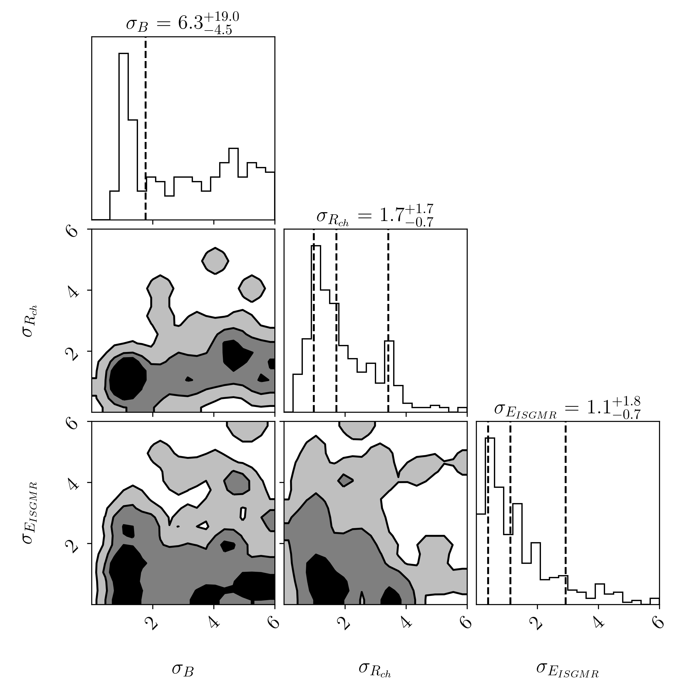
We show in Fig. 2 the distribution of the rms deviations associated with the observables , and , for all the interactions considered (415 in total). Note that for these three observables, the main peak is systematically located at about , which supports our choices for the associated uncertainties presented in Section II.
In the following, we sort the modeling according to the rms deviation and attribute to them a set of letters, namely the three letters for the groups Gi and the five letters for the groups Di, where the letters are:
- •
, if ;
- •
, if ;
- •
, if ;
- •
, if .
The complete list of the scores for each parametrization analyzed in this work is given in the supplemental material. As examples, we obtain the following scores for the two approaches (global versus detailed) in the cases of the relativistic NLSV1, and the non-relativistic RATP and SLy4 Skyrme forces:
- •
NLSV1: ABC, BA:AB:C,
- •
RATP: BBA, BC:BB:A,
- •
SLy4: BBA, BB:BB:A.
The relativistic NLSV1 interaction reproduces the binding energies better than the charge radii, which are better reproduced than the ISGMR energy. In detail, the binding energies (charge radius) of the nuclei are better (worse) reproduced than the ones. For the non-relativistic models, we observed that they are scored identically (BBA) in the general analysis, but a more detailed analysis shows that the SLy4 is better than the RATP at reproducing the binding energies in nuclei. This illustrates the differences in the global and detailed approach, which will be further analysed in the following.
| D0/G0 | D1 | G1 | D2 | G2 | D3 | G3 | D4 | G4 | D4sym | |
|---|---|---|---|---|---|---|---|---|---|---|
| Total | 374 | 81 | 90 | 66 | 74 | 61 | 74 | 45 | 54 | 22 |
| MM⊙ | 312 | 77 | 85 | 65 | 72 | 61 | 72 | 45 | 52 | 22 |
| MM⊙ | 198 | 49 | 53 | 44 | 49 | 41 | 49 | 25 | 29 | 12 |
Based on the criteria described above, we separate the interactions submitted to the finite nucleus constraints into five different groups, as follows,
- •
D0 and G0: groups containing all the interactions considered,
- •
D1 and G1: groups containing interactions with a letter rank from to over all types of data,
- •
D2 and G2: groups containing interactions with a letter rank of or for the binding energies,
- •
D3 and G3: groups containing interactions with a letter rank of or for the binding energies and charge radii,
- •
D4 and G4: groups containing interactions with a letter rank of or for the binding energies, charge radii and GMR energies.
- •
D4sym: This group imposes on top of D4 the constraint “IAS+”, as detailed in the following.
The number of interactions surviving the conditions imposed on the different groups Di and Gi are shown in Table 4 by the line denoted by “total”. We also count the number of interactions that permit a neutron star of mass MM⊙ and MM⊙ in the case of TOV hydrostatic equilibrium, as is detailed in the following Section IV. We remark that the D0 (or G0) group is composed of parametrizations rather than , the total number of interactions. This is due to the fact that a number of problematic interactions have been discarded, due to one of the following conditions: (i) spinodal instability (negative values of the sound speed) above or (ii) negative value of the pressure in stellar matter.
III.2 Impact of the groups and on the - correlation
We compare in Fig. 3 the impact of the different groups Gi and Di on the - correlation. It is clear that the groups Di are better correlated than the groups Gi, reflecting the constraint that and nuclei are reproduced with same accuracy. Already the group D2 is better correlated than the group G2, showing that the goodness of the models to reproduce data (the difference between G1 and G2 or D1 and D2) is less effective than the condition imposed on the D2 models (difference between D2 and G2). The additional condition also appears through the charge radii, i.e. D3 removes the lower values of , while the additional constraint on the ISGMR in 208Pb plays a small but non-negligible role (difference between D3 and D4).
By comparing the contours G4 with D4, we see clearly the impact of imposing that and nuclei are reproduced with the same accuracy. In G4 for instance, a poor reproduction of nuclei could be compensated by a better description of ones, e.g., as occurs for the SKa interaction. This is not true in the group D4, which creates a tighter correlation in the - diagram, see bottom panel in Fig. 3.
In conclusion, Fig. 3 shows the effectiveness of the condition that and nuclei are reproduced with same accuracy on the - correlation. The constraints on the charge radii and ISGMR centroid energy also play an additional role for the Di groups, but have almost no impact on the Gi groups.
III.3 The group D4sym with an additional symmetry energy constraint
We now detail how the group D4sym, see Table 4, is obtained by adding symmetry energy constraints on top of the D4 group, which has been shown in Section III.2 to naturally constrain and . Among the set of experimental constraints for the symmetry energy shown in Section II.5, we decided to investigate the impact of IAS+ Danielewicz2013 since it is obtained from low-energy nuclear data. Another reason for investigating these constraints is that they are provided as contours in the density dependence of the symmetry energy, see Fig. 4. We can then filter our interactions in the D4 group according to their ability to fit inside these contours, as illustrated in Fig. 4.
Two contours are shown in Fig. 4: the one representing the IAS constraint alone as well as one representing the IAS+ constraints together. The different colors reflect the different kinds of interactions analyzed, namely, black for Skyrme, blue for RMF-NL, and red for RMF-DD. For each model, we compute a loss function defined as , where the index to scans over the data. Models with are accepted. The interactions compatible with the IAS + constraint are represented by dashed curves and define the D4sym group.
We now show in Fig. 5 the region of the - which is populated by the D4sym group. For a better understanding, we also show the role of the groups D0, D4, D4+IAS and finally D4sym. The contour D4 isolates a subgroup allowed by HIC and is partially excluded by the unitary gas constraint. We show how the constraint from IAS (D4+IAS) and IAS + (D4sym) Danielewicz2013 reduces the viable models shown in the - diagram. Including the IAS constraint (D4+IAS) reduces the contour to a smaller group which makes it compatible with neutron stars, and finally the contour D4sym reduces it even further inside the (Sn) experimental constraint. All the new contours (D4, D4+IAS and D4sym) are given in the supplemental material.
One could also remark that, despite the good overlap between the IAS experimental constraint and our D4+IAS contour, some of our interactions are outside the IAS experimental constraint. This is because we have considered a larger number of interactions, including relativistic approaches, which haven’t been considered in Ref. Danielewicz2013 where the contours are based on results solely from Skyrme models. The same remark could be made about the comparison of the group D4sym and the IAS+ experimental constraint.
| group | ||
|---|---|---|
| (MeV) | (MeV) | |
| D4 | 33.52.4 | 73.423.3 |
| D4+IAS | 32.31.2 | 62.912.3 |
| D4sym | 31.80.7 | 58.19.0 |
Finally, the centroid and the standard deviation evaluated among the interactions forming the groups D4, D4+IAS and D4sym are given in Table 5. Note the small dispersion obtained for the D4sym group.
IV Masses and radii of neutron star
We now reach the second stage of our analysis where the EDFs that have been successfully selected by their goodness in reproducing finite nuclei properties are confronted with their predictions for NS properties. The EoS for dense matter and NS are detailed in Appendix C. In this section, we discuss their predictions.


The properties of non-rotating NS are obtained from the solution of the the Tolman-Oppenheimer-Volkoff (TOV) equations tov39; tov39a; glen written as ()
| (28) | ||||
| (29) |
whose solution is determined by the initial conditions (central pressure) and . In Eqs. (28) and (29), the energy density and pressure are given from Eqs. (60)-(61). The maximum value of for a given EoS is called MTOV. The radius corresponding to a given mass, e.g., M⊙, is called .
The break-down density above which the nucleonic EoS is replaced by an EoS with new degrees of freedom, e.g. hyperons or quarks, is not known. Turning the discussion of the break-down density into NS masses is easier in terms of observational data. For instance, a NS with mass M⊙ corresponds to central densities of 1.7-3/2-4.5/2.3-6, where the larger central densities are obtained for the softer EoSs. From these numbers, it is reasonable to extrapolate the nucleonic EoS up to about M⊙, while the NS with M⊙ are considered as an extreme nucleonic scenario. In the following, we explore two cases where MM⊙ and MM⊙.
At very low mass (below M⊙) the core EoS is connected to a crust EoS. The necessity of having a unified approach for both the crust and the core DH2001; fortin has been pointed out. Nevertheless, a piece-wise approach, in which the EoS in the core is connected to another EoS in the crust, is also widely used when a precision in the NS radius of about 100 m is sufficient or when detailed information of the crust-core transition is not required. In this work we adopt the procedure used in Refs. Margueron2018b in which the SLY interaction of Ref. DH2001, based on the SLy4 Skyrme parametrization Chabanat1998, is used for the crust region up to . As in Refs. Margueron2018b, a uniform matter EoS starts at and a log scale cubic spline takes care of smoothly connecting the lower limit of the crust to the upper limit of the core. Such a prescription allows a good description of the crust and the core, provided they can be smoothly connected. Exceptions exist however. For instance if the core EoS is described by an interaction with a value for much larger than the one used to describe the crust, difficulties in connecting the pressure in the crust and the core regions appear. This, however, is not the case for the interactions selected in the D4 group.
Mass-radius profiles are shown in Fig. 7 for various sets of EoSs. The condition MM⊙ removes a small region in the MR diagram corresponding to the softer EoSs for which MM⊙. We represent the individual contributions of the interactions belonging to the D4 group with the same convention as detailed in Fig. 4. Dashed curves represent the interactions satisfying this constraint, namely, black for Skyrme, and blue for RMF-NL interactions with constant coupling constants. In the bottom panels of Fig. 7, the envelopes of the groups D4 (dark brown) and D4sym (green) are compared. The stiffest EoSs from the D4 group are excluded in the D4sym group, since they require a symmetry energy out of the boundaries shown in Fig. 4. We obtain (12.53) km for the D4 (D4sym) group for MM⊙ and (12.38) km for MM⊙.
The contours related to the observational constraints from NICER nicer1a; nicer1b; nicer2a; nicer2b and for the GW170817 event detected by LIGO and Virgo Collaboration ligo are indicated in the bottom panels. A good overlap between the NICER contours and the groups D4 and D4sym is obtained, illustrating the agreement between the present constraints from nuclear physics and the ones from observations of neutron stars. A similar conclusion was obtained in Ref. Tews2018 for the gravitational waves constraint extracted from GW170817.
We now perform a more detailed study of the different groups Di and Gi ( to 4) to understand the impact of the different low energy nuclear constraints we have considered. In Fig. 8, we compare the largest radius uncertainty , namely, the difference between the maximum and the minimum radius, with the standard deviation defined as
| (30) |
where runs over the nuclear interactions belonging to the groups Di (solid lines) or Gi (dashed lines). As expected, we have and both quantities increase as functions of the mass. For a canonical mass NS and the D4 group, we obtain km and km (assuming only that MM⊙). The number of interactions belonging to each group is given in Table 4. Comparing D1/G1 and D2/G2 one measures the impact of better accuracy in the reproduction of the masses: the impact is very small in general. Note however a small reduction of between G1 and G2 at the mass 1.6M⊙. Then, comparing D2/G2 and D3/G3 as well as D3/G3 and D4/G4, one can see the successive impact of an improved reproduction of the charge radii and ISGMR. Note the reduction of induced by the condition on the charge radius in the groups , which is not visible for the groups . This shows that the requirement to reproduce the charge radius in and with the same accuracy is the main condition which breaks the degeneracy between the groups and .
The striking result from Fig. 8 is however the very weak dependence of the radius uncertainty, represented here by and , across the increasing index of the groups Di and Gi. This feature indicates that a more accurate reproduction of experimental masses, charge radii and the GMR energy in 208Pb does not have a major impact on the modelling of global NS properties, here M and R. There is however still an impact from the requirement that and nuclei are described with same accuracy, which is mainly given by the charge radius data.


Our finding suggests that a rough reproduction of low-energy nuclear physics properties (experimental masses, charge radii and ISGMR energy), as given in model D4 for instance, is sufficient, provided that and nuclei are described with same accuracy. The gain in improving the modeling reproducing these experimental data is not effective for the prediction of NS global properties. The reason is that the extrapolation from finite nuclei located at around and close to isospin symmetry to canonical mass NS with densities above , where matter is neutron rich , requires the knowledge of the density and isospin dependence of the nuclear EoS, which represents a large and effective source of uncertainties. However, low-energy nuclear physics properties should be more important in determining the properties of the crust, such as the mass and the charge of nuclear clusters (, ), see for instance Refs. Wolf2013; Fortin2016; Antic2019; Grams2022a; Grams2022b.
V Further analysis of the density dependence of the symmetry energy
In the previous section, we illustrated the needs for a better understanding of the density dependence of the nuclear EoS for the prediction of NS global properties. Since the symmetry energy is the most important term in the EoS driving the density dependence of the EoS and since the quadratic nuclear empirical parameters (QNEPs) allow for a simple representation of this density dependence, we now analyse directly the QNEPs.
We present the normalized distributions (ND) of the QNEPs , , , and in Fig. 9 for various scenarios. We also present the prior distribution represented by the black dashed lines. This prior is obtained from the D0 group.

The positions of the ND peaks for are almost identical to that of the prior, showing no effect of the interaction selection or the condition on MTOV for this QNEP. The ND for the group D4sym is more peaked than the others. For , the prior is almost flat while the posterior distributions indicate a preference for lower values of (about 50-70 MeV). In the case of group D4sym, the normalized distribution is double peaked, as is the distribution for . For the latter, one maximum is located in the region to MeV and another around MeV. With regard to the D4 group, notice that the relative size of the peaks in changes with the mass constraint: the peak at -100 MeV is preferred if MMTOV, while the peak around 0 MeV is preferred if MMTOV. For , the PDF is very broad, with most of the models lying between 100 an 600 MeV. The centroid of the normalized distribution conditioned by MM⊙ is, however, larger than the one conditioned by MM⊙. This shows that both and are impacted by the condition on MTOV.
| D0 | DD | D | |
|---|---|---|---|
| 5.75 – 160.06 | 45.36 – 126.60 | 45.36 – 73.23 | |
| -393.73 – 159.57 | -121.90 – 132.12 | -121.90 – 12.96 | |
| -786.14 – 1361.45 | -166.17 – 776.91 | 128.26 – 524.75 | |
Another view of these data is shown in Fig. 10, where we plot the correlations between the QNEPs ( versus in the top panels and versus in the bottom panels) for interactions in the D0 group (left panels) and D4 groups central and right panels. These two last cases also show the impact of MTOV. We observe that there are no strong correlations among the QNEPs visible in this figure. The reason is that a low value of could be compensated by larger values of and/or . There is however a set of limits that we can extract from Fig. 10. This set is given in Table 6.
The lower boundary in is due to two constraints. The first one is the reproduction of the low-energy nuclear physics properties, which produces a lower limit of the order of 30 MeV, as shown in Fig. 9. The requirement to reproduce large masses, such as or pushes this lower limit up to about 45 MeV. It is however important to keep in mind that the boundaries we obtain are strongly impacted by the hypothesis that we have made concerning the absence of phase transition above saturation density. The case of a phase transition has been studied in Ref. Xie2021.
The range of values for the isovector QNEPs reported in Table 6 could however be compared to other boundaries suggested in the literature. In the following we assume that the NEPs and QNEPs in the isospin channel are similar. For instance, by analysing non-relativistic Skyrme, relativistic mean field and relativistic Hartree-Fock models, it has been suggested that MeV Margueron2018a. From observational constraints based on X-ray emission from seven NSs in globular clusters, a value MeV was preferred Baillot2019. These values are consistent with the recent analysis based on GMR energies in 90Zr, 116Sn and 208Pb using the Skyrme model, leading to MeV Sagawa2019. From the analysis of GW170817, it was suggested that MeV Carson2019 and, in a similar analysis, the following values were suggested Guven2020 MeV, MeV, and MeV, depending on the observational PDF for extracted from GW170817 Abbott2019; De2018; Coughlin2019. The value taken for , however, was shown to be well anti-correlated with , mainly driven by the condition to reproduce 2M⊙. Since the PDFs for from GW170817 prefer low values for , this explains why large values for were obtained in Ref. Guven2020. More recently, a compilation of 16 results from independent analyses of neutron star observational data since GW170817 lead to the following expectation, MeV Li2021. We also mention a recent analysis based on the latest results from the NICER observatory, where it was found that the lower radius limit of J0740 by Riley et al. nicer2b only requires to be higher than about MeV, depending somewhat on the value of the skewness of the symmetry energy (unconstrained by the data).
All these results have to be taken with caution however, since they have been obtained with different nuclear models and corresponding systematical uncertainties that are difficult to estimate. Different priors have also been considered for the results based on a Bayesian statistical approach, which impact the results. We note, however, that our present findings for are in agreement with the predictions from these analyses.
In conclusion, we have extracted constraints on the QNEPs determining the density dependence of the symmetry energy. These constraints are given in Table 6 for the different groups: D0, D4 and D4sym conditioned by MTOV. One could remark that these QNEPs are still largely unknown, although they are crucial for precise predictions of NS properties. However, the ranges for these QNEPs given in Table 6 represent the best evaluation of these QNEPs based on low energy nuclear experiments and conditioned by MTOV.
VI Neutron star global properties
In this section we further elaborate on the role of the symmetry energy in the determination of NS global properties. We then introduce a refined classification of the EDFs based on the properties of the symmetry energy and we analyse the impact of this classification on NS global properties.
VI.1 Mass-radius relation of neutron stars
The mass-radius (MR) relations for the interactions of the group D4 are shown in Fig. 11, in a similar manner as in the top panels of Fig. 7. In addition, we have grouped the interactions in D4 into six different sets according to their MR relations. These sets are shown in color as indicated in the legend.
| D4sym | interaction | Ref. | ||||||||||||||
| I | SLy3 | Chabanat-thesis | 0.160 | -15.94 | 229.51 | -362.56 | 31.97 | 45.36 | -121.90 | 524.75 | 107.61 | 162.18 | -322.39 | 0.70 | ||
| SLy4 | Chabanat1998 | 0.160 | -15.97 | 229.91 | -363.11 | 32.00 | 45.94 | -119.73 | 521.53 | 110.18 | 158.43 | -322.83 | 0.69 | |||
| SLy230b | Chabanat1997 | 0.160 | -15.97 | 229.91 | -363.10 | 32.01 | 45.97 | -119.72 | 521.50 | 110.19 | 158.40 | -322.92 | 0.69 | |||
| SLy0 | Chabanat-thesis | 0.160 | -15.97 | 229.66 | -364.01 | 31.98 | 47.11 | -116.23 | 508.68 | 113.43 | 144.67 | -324.23 | 0.70 | |||
| SLy8 | Chabanat-thesis | 0.160 | -15.97 | 229.89 | -363.27 | 32.00 | 47.18 | -115.59 | 509.88 | 114.31 | 146.61 | -324.09 | 0.70 | |||
| SLy2 | Chabanat-thesis | 0.161 | -15.99 | 229.92 | -364.21 | 32.00 | 47.46 | -115.13 | 506.52 | 114.79 | 142.31 | -324.69 | 0.70 | |||
| SLy5 | Chabanat1998 | 0.161 | -15.99 | 229.92 | -364.16 | 32.01 | 48.15 | -112.76 | 500.67 | 117.16 | 136.51 | -325.38 | 0.70 | |||
| II | SD1 | sd1 | 0.156 | -15.70 | 231.91 | -376.39 | 32.00 | 60.94 | -115.87 | 281.29 | 116.04 | -95.10 | -382.59 | 1.00 | ||
| III | IUFSU* | iufsus | 0.150 | -16.02 | 235.67 | -259.49 | 29.85 | 50.30 | 12.20 | 388.15 | 247.87 | 128.67 | -234.20 | 0.61 | ||
| SINPA | sinpab | 0.151 | -16.00 | 202.55 | -58.73 | 31.20 | 53.85 | 26.58 | 334.85 | 229.13 | 276.12 | -280.92 | 0.58 | |||
| BSR8 | BSR | 0.147 | -16.04 | 230.95 | -290.85 | 31.08 | 60.25 | -0.74 | 238.23 | 230.22 | -52.62 | -286.36 | 0.61 | |||
| BSR15 | BSR | 0.146 | -16.03 | 226.82 | -512.29 | 30.97 | 61.79 | -21.36 | 128.26 | 205.47 | -384.03 | -252.54 | 0.61 | |||
| FSUGZ06 | fsugz | 0.146 | -16.05 | 225.06 | -503.17 | 31.18 | 62.42 | -24.49 | 153.31 | 200.57 | -349.86 | -259.47 | 0.61 | |||
| BSR16 | BSR | 0.146 | -16.05 | 224.98 | -503.17 | 31.24 | 62.33 | -24.17 | 152.29 | 200.82 | -350.88 | -258.75 | 0.61 | |||
| BSR9 | BSR | 0.147 | -16.07 | 232.50 | -297.11 | 31.61 | 63.89 | -11.32 | 202.86 | 221.18 | -94.25 | -313.03 | 0.60 | |||
| FSUGZ03 | fsugz | 0.147 | -16.07 | 232.48 | -297.13 | 31.54 | 63.98 | -11.66 | 203.43 | 220.82 | -93.69 | -313.79 | 0.60 | |||
| BSR17 | BSR | 0.146 | -16.05 | 221.67 | -489.45 | 31.98 | 67.44 | -31.58 | 176.65 | 190.09 | -312.80 | -287.31 | 0.61 | |||
| BSR10 | BSR | 0.147 | -16.06 | 227.41 | -255.13 | 32.72 | 70.83 | -16.51 | 205.04 | 210.89 | -50.09 | -362.04 | 0.60 | |||
| SINPB | sinpab | 0.150 | -16.05 | 206.40 | -449.21 | 33.96 | 71.55 | -50.60 | 552.47 | 155.80 | 103.26 | -449.21 | 0.59 | |||
| BSR18 | BSR | 0.146 | -16.05 | 221.13 | -485.73 | 32.74 | 72.65 | -42.24 | 199.39 | 178.89 | -286.35 | -318.55 | 0.61 | |||
| SKa | ska | 0.155 | -15.99 | 263.16 | 300.13 | 32.91 | 74.62 | -78.46 | 174.54 | 184.70 | 474.66 | -441.08 | 0.61 | |||
| BSR12 | BSR | 0.147 | -16.10 | 232.35 | -290.31 | 34.00 | 77.90 | -44.23 | 324.15 | 188.12 | 33.85 | -414.30 | 0.61 | |||
| BSR11 | BSR | 0.147 | -16.08 | 226.75 | -312.37 | 33.69 | 78.78 | -24.72 | 172.54 | 202.03 | -139.83 | -388.86 | 0.61 | |||
| BSR19 | BSR | 0.147 | -16.08 | 220.83 | -484.25 | 33.78 | 79.47 | -50.13 | 194.70 | 170.70 | -289.55 | -352.70 | 0.61 | |||
| BSR20 | BSR | 0.146 | -16.09 | 223.25 | -507.75 | 34.54 | 88.03 | -39.90 | 82.74 | 183.35 | -425.02 | -367.86 | 0.61 | |||
| BSR13 | BSR | 0.147 | -16.13 | 228.64 | -294.46 | 35.82 | 91.07 | -41.68 | 138.98 | 186.96 | -155.48 | -470.82 | 0.60 | |||
| BSR21 | BSR | 0.145 | -16.12 | 220.32 | -468.20 | 35.96 | 92.94 | -46.01 | 67.45 | 174.30 | -400.75 | -406.16 | 0.60 | |||
| BSR14 | BSR | 0.147 | -16.18 | 235.47 | -317.10 | 36.32 | 93.85 | -41.95 | 112.53 | 193.51 | -204.57 | -478.66 | 0.61 | |||
| IV | FSUGarnet | fsugarnet | 0.153 | -16.23 | 229.61 | -13.12 | 30.92 | 50.96 | 59.44 | 138.08 | 289.06 | 124.96 | -249.21 | 0.58 | ||
| DD-ME2 | ddme2 | 0.152 | -16.14 | 250.92 | 478.75 | 32.30 | 51.25 | -87.19 | 776.91 | 163.73 | 1255.67 | -492.45 | 0.57 | |||
| DD-ME1 | ddme1 | 0.152 | -16.20 | 244.72 | 316.66 | 33.06 | 55.45 | -101.05 | 705.59 | 143.66 | 1022.25 | -505.50 | 0.58 | |||
| BSR1 | BSR | 0.148 | -16.02 | 239.89 | -35.68 | 31.04 | 59.41 | 12.96 | 468.10 | 252.85 | 432.42 | -334.65 | 0.61 | |||
| BSR2 | BSR | 0.149 | -16.03 | 239.93 | -48.06 | 31.50 | 62.02 | -3.14 | 403.21 | 236.79 | 355.15 | -362.81 | 0.61 | |||
| FSUGZ00 | fsugz | 0.149 | -16.03 | 240.00 | -47.74 | 31.43 | 62.16 | -3.46 | 402.48 | 236.54 | 354.74 | -364.05 | 0.61 | |||
| BSR3 | BSR | 0.150 | -16.09 | 230.55 | -114.72 | 32.74 | 70.45 | -7.76 | 397.59 | 222.78 | 282.86 | -395.42 | 0.60 | |||
| BSR4 | BSR | 0.150 | -16.08 | 238.57 | 4.00 | 33.17 | 73.23 | -20.71 | 420.06 | 217.85 | 424.06 | -461.34 | 0.61 | |||
| BSR5 | BSR | 0.151 | -16.12 | 235.71 | -10.96 | 34.46 | 83.37 | -14.16 | 346.84 | 221.55 | 335.88 | -510.53 | 0.61 | |||
| BSR6 | BSR | 0.149 | -16.13 | 235.75 | -7.59 | 35.62 | 85.68 | -49.55 | 352.00 | 186.20 | 344.41 | -560.86 | 0.60 | |||
| BSR7 | BSR | 0.149 | -16.18 | 231.80 | -19.80 | 37.26 | 99.14 | -16.97 | 198.47 | 214.83 | 178.66 | -603.32 | 0.60 | |||
| V | FSUGold2 | fsugold2 | 0.150 | -16.26 | 237.69 | -149.95 | 37.57 | 112.68 | 25.38 | -166.17 | 263.07 | -316.13 | -579.61 | 0.59 | ||
| VI | Q1 | q1 | 0.148 | -16.10 | 241.86 | 8.70 | 36.44 | 115.71 | 105.65 | 266.72 | 347.51 | 275.43 | -592.77 | 0.60 | ||
| FAMA1 | fama1 | 0.148 | -16.00 | 200.05 | -303.20 | 38.01 | 120.53 | 113.22 | 403.17 | 313.27 | 99.97 | -427.27 | 0.60 | |||
| NL3* | nl3s | 0.150 | -16.31 | 258.25 | -122.04 | 38.68 | 122.63 | 105.56 | 223.95 | 363.81 | 101.92 | -688.19 | 0.59 | |||
| E | eer | 0.150 | -16.13 | 221.43 | 20.87 | 38.58 | 124.57 | 132.12 | 381.38 | 353.54 | 402.25 | -627.06 | 0.58 | |||
| ER | eer | 0.149 | -16.16 | 220.49 | -24.93 | 39.42 | 126.60 | 127.62 | 377.17 | 348.11 | 352.24 | -617.67 | 0.58 |
These sets could also be sorted by the values of the NEPs , and the condition that MM⊙ as shown in table 7: set I consists of interactions from the group D4 for which MeV; set II, III and IV have , and additionally set II contains the single EoS for which MeV, while sets III and IV have larger values for MeV. The difference between set III and IV is that all EoSs from set IV satisfy the condition MM⊙, while models in set III do not, except for the SKa parametrization. Finally, sets V and VI are EoSs with large values for MeV. Set V has a value of of about MeV, while set VI has MeV.
The analysis of Fig. 11 and Table 7 leads to the following conclusions: The main difference among the different sets is coming from the value of : low values (set I), intermediate values (sets II, III and IV) and large values (set V and VI). The value of determines the stiffness of the EoS as shown in Fig. 11: the softer the EoS, the lower the radius and the larger the central density for a given mass M. To a certain degree, the stiffness of the EoS is determined by the value of . In order to make this more clear in Fig. 11, we have separated set II from sets III and IV according to the value of .
We also indicate in Table 7 the EoSs which belong to the subgroup D4sym. They are the EoSs for which MeV. Note that the precise upper value for actually depends on the value of .
In conclusion, we have analysed the dominant role of in globally controlling the MR diagram, with some additional contribution from . In Fig. 11 however, one observes some correlations between and the masses/radii at fixed central densities. In the following, we analyse these correlations in more detail.
VI.2 Radius and mass (individual analysis)
We represent in Fig. 12 the correlation between the NS radius R – extracted at different densities (, and ) – and . Note that the correlation is opposite at to that at higher densities: At the radius decreases as increases, while above, the radius increases as a function of . The reason is simple: having a larger value of implies a softer EoS below . So the anti-correlation at reflects that the EOS is softer at low densities for larger values of . At higher densities, the situation is different since the larger the value of , the stiffer the EoS is above . The EoSs are so stiff that they change the MR relation: above saturation density, the radius is weakly impacted by the mass. Since stiffer EoSs above imply larger values for , the radius is correlated with in this region.
We now test the empirical relation between R and , suggested in Ref. Prakash2001. The pressure is the central pressure of the NS (at -equilibrium). We show the quantity as a function of in Fig. 13. The correlation between R and is better at and compared to , as already noted in Ref. Prakash2001. The product is weakly correlated with the radius, if the pressure is taken at and . Since the radius is well correlated with at these densities, see Fig. 12, the product is also weakly correlated with at and . At however, the points are much less aligned than at and . The dispersion between the points reflects the (dominant) effect of as well as that of . In NS, the central pressure near saturation density is dominantly given by Lattimer2016, while other NEPs contribute more as the density increases Margueron2018a; Margueron2018b.
The correlation suggested in Ref. Prakash2001 at and reflects at least two interesting features: first it shows the weak influence of the radial distribution of the pressure in NSs, since it is mostly the central value which fixes the NS radius, and second, it hides the contribution of the different NEPs to the density dependence of the pressure, since the correlation furnishes the central pressure directly.
With regard to the correlation between NS mass and , notice that in Fig. 11 one observes the relation between the mass M at fixed central density and the radius, which reflects the influence of . To make this clearer, we explicitly represent in Fig. 14 the correlation between the mass M and at different central densities: , and . The correlation is almost perfect at with the correlation coefficient being 0.995 (0.998) for MM⊙ (MM⊙). However, it becomes broader at higher densities. This reflects the role of other empirical parameters governing the density dependence of the EoS, as for instance or . It is also interesting to observe that the correlations are very close for and 2 when conditioned by MM⊙ in comparison to the MM⊙ case, reflecting the weak impact of MTOV on this correlation. The same is not true for 3, that presents a better correlation when the 2MM⊙ condition is applied.
VII Other global properties of neutron stars
In this last section of the paper, we analyse global properties of NS that have not yet been analysed, namely the moment of inertia and the tidal deformability.
VII.1 Moment of inertia
In the low spin regime, as suggested by Hartle and Sharp inertia1, the rotation of a NS is much smaller than the Kepler frequency, allowing us to assume that the NS remains spherical. The moment of inertia is therefore expressed as inertia1; inertia2
| (31) |
where is the local spin frequency, which represents the correction from general relativity to the asymptotic angular momentum . The local angular momentum is . Furthermore, and is the gravitational potential solution of the equation
| (32) |
with the boundary condition .


We then investigate how the moment of inertia is influenced by the low energy nuclear experimental constraints. We show in the top panels of Fig. 15 the moment of inertia as a function of the mass M for the six sets, as indicated in the legend. There is a reasonable ordering of the moment of inertia as a function of the sets: the moment of inertia increases for increasing values of . We obtain (1.24) g.cm2 for the D4 (D4sym) group for MM⊙ and (1.22) g.cm2 for MM⊙.
A more systematical investigation of the moment of inertia is shown in Fig. 16, where the effects of the groups D1-D4 and G1-G4 are given in the four panels. As in Fig. 8, we represent the largest uncertainties and the standard deviation . The uncertainty measured by these two quantities increases as a function of the mass M. We also confirm our previous conclusions from Fig. 8: there is only a very limited impact due to a better description of the low-energy nuclear data. An improvement is seen when using the Di groups rather than the Gi ones, showing that the condition to describe equally well the and nuclei also plays a role here. However, the uncertainty in the moment of inertia is generated by the unknown density dependence of the EoS, as we have already discussed in the case of the radius.
VII.2 Tidal deformability
Finally, we address the question of the tidal deformability, which is probed by coalescing neutron stars and carried away by gravitational waves emitted during the last orbits before merger. We analyse its correlation with the experimental nuclear data.

Tidal deformability is defined as the quotient of the induced quadrupole moment to the tidal field . In terms of the second Love number , it is given by . One can also define the dimensionless tidal deformability as where is the compactness. The Love number is defined as,
| (33) | |||||
with and being the solution of the differential equation,
| (34) |
where the functions and are given by
| (35) | |||||
| (36) | |||||
in which is the square of the sound speed and tanj10; Prakash; hind08; damour; tayl09; had4.
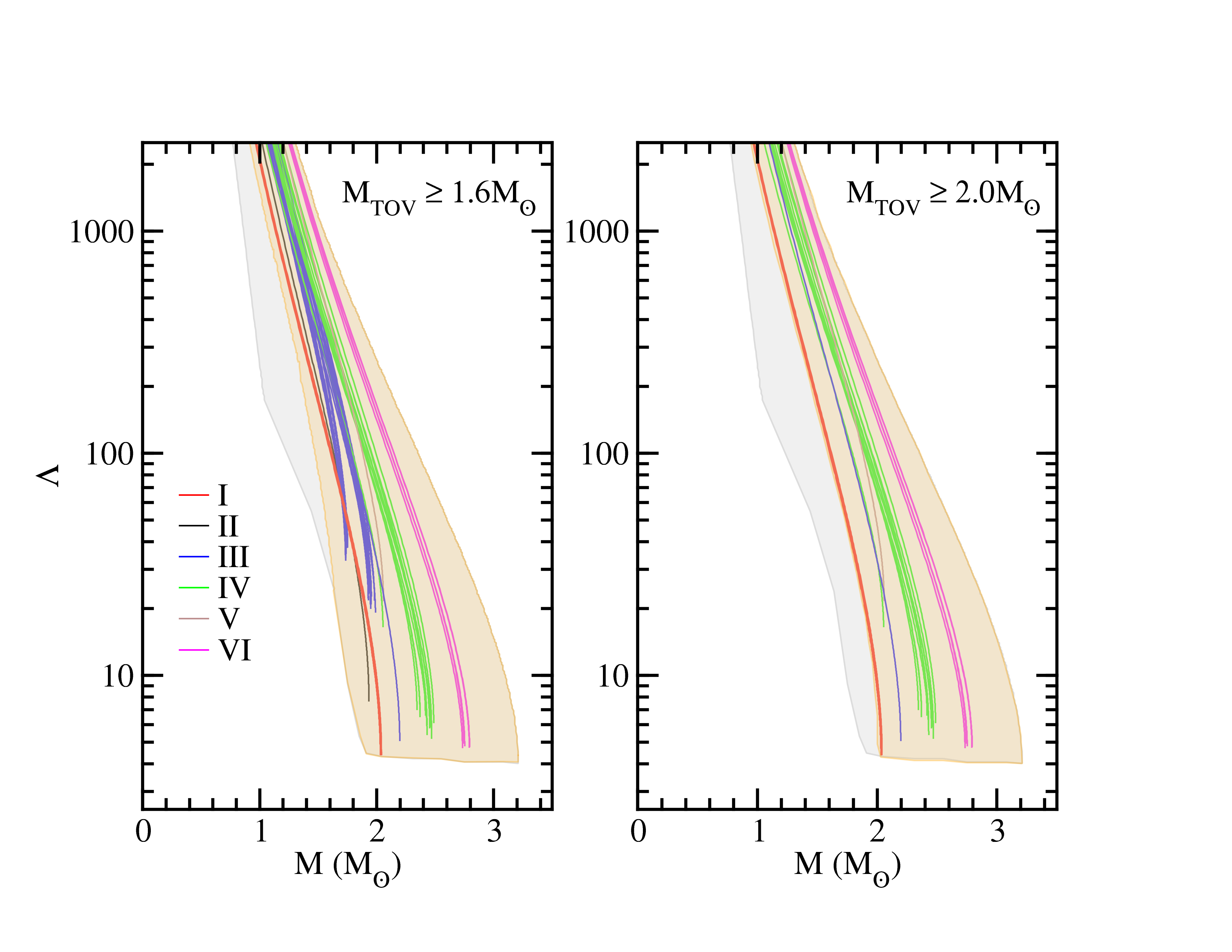
The dimensionless tidal deformability is shown as a function of M in Fig. 17 for the six sets, as indicated in the legend. We can compare the envelop of the best EoS (group D4) with the prior from group D0 (grey band). The orange band represents the envelop of the group D0 conditioned by the constraint on MTOV. As discussed previously for the M-R relation, as well as for the I-R one, there is only a small impact of a better reproduction of the low-energy nuclear data, with most of the uncertainty originating from the unknown density dependence of the EoS. We also indicate the point reported by the LIGO/Virgo collaboration for the dimensionless tidal deformability of a canonical star, namely, ligo. As we see, the softest interactions are more compatible with this specific restriction. We obtain (482) for the D4 (D4sym) for MM⊙ and (474) for MM⊙.
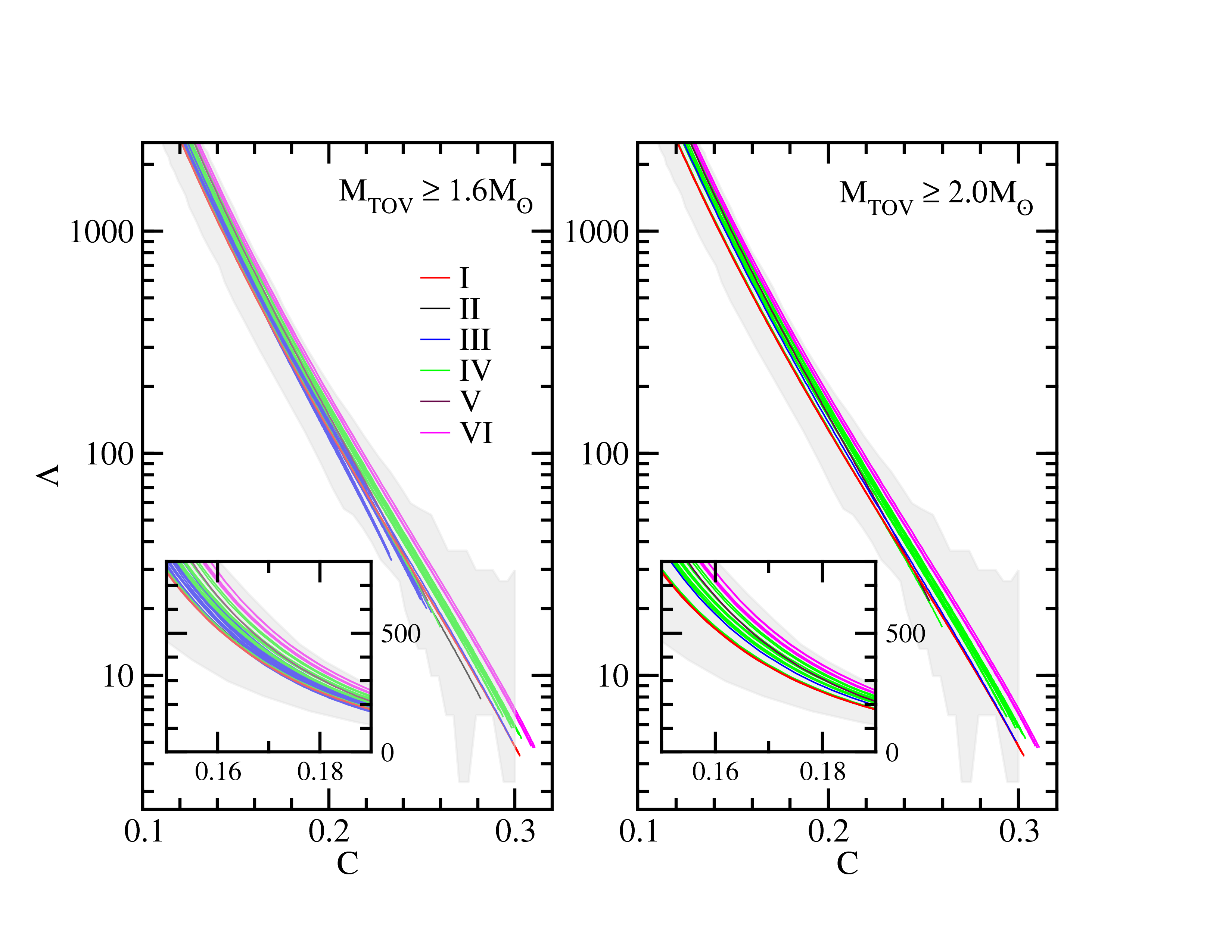
We investigate in Fig. 18 the - universal relation suggested in Ref. Yagi2014. The contributions for the six sets are shown in different colors. We confirm the universal relation, and we show that the dispersion in this relation is mainly given by . In addition, the dispersion is even larger when all EDFs in the D0 group are considered. The origin of the small dispersion is thus due to the interaction selection of the Gi/Di groups. We have checked that an accurate description of the low-energy nuclear data by the EDFs is also less important here than an improved determination of the density dependence of the EoS.
In Fig. 19 we present the maximal uncertainty and the standard deviation related to the dimensionless tidal deformability, defined similarly to the moment of inertia and to the radius shown before. We clearly see a reduction of and as a function of the neutron star mass, at variance with the analysis of R and I. This is related to the fact that is strongly decreasing with M, as shown in Fig. 17. The correlation of the experimental nuclear data with the tidal deformability is extremely small. Among the quantities we have investigated in this study, the tidal deformability is perhaps the quantity on which the constraints provided by the experimental nuclear data has the smallest impact.
Finally, we show in Fig. 20 the dimensionless tidal deformability of a M=M⊙ star, namely, , as a function of the NEPs , , and . This figure is similar to Fig. 5 from Ref. Wei2020, which showed no correlation for a reduced set of nuclear interactions. From this figure, the authors of Ref. Wei2020 concluded that there is no correlation between global properties of NS and saturation properties of nuclear matter. We find that a correlation does indeed exist, when considering the D4 group conditioned by MTOV. We find a good correlation for - and - for the D4 group with both constraints on MTOV. In the case of the D4sym subgroup, we see that the correlation of with n longer exists, but for there is still a correlation, although smaller than for the D4 group. Concerning -, we find the Pearson correlation coefficients to be smaller than in all cases. We thus conclude that correlations do exist between global properties of NSs and saturation properties, especially for the isovector QNEPs, although there is a large dispersion in these correlations, which limits the value of the Pearson correlation coefficient.
VIII Conclusions
In this study, we have analysed the link between the constraints on mean field EDFs generated by low-energy nuclear experimental data and their corresponding predictions for NSs. To do so, we have investigated 415 mean field interactions, both relativistic and non-relativistic, for which we have calculated several quantities that can be directly compared to the experimental data. These quantities are the masses, radii and GMR energies of a number of doubly magic nuclei (chosen to minimize the impact of uncontrolled approximations such as pairing, deformation, etc). We have defined five groups, from G0 to G4, where G0 is the set of interactions reproducing the experimental nuclear masses with the largest tolerance, G2 with the smaller tolerance, while G3 and G4 add successively the constraint on the charge radius and the giant monopole resonance. In these groups, we have evaluated the reproduction of the experimental data globally. They are contrasted with another set of groups, called D0 to D4, for which a more detailed evaluation is performed by separating the nuclei from the others: To be well ranked in the groups Di, the interactions must reproduce equally well the and nuclei. From this first step of our analysis, we find that
- 1.
The group D4 exhibits a fairly strong correlation between and .
- 2.
By combining the low-energy nuclear data and an analysis of the density dependence of the symmetry energy Danielewicz2013, we have isolated a group D4sym that further reduces the uncertainty in the symmetry energy. We find MeV and MeV.
In a second step, we have confronted the different groups Gi and Di with global observational quantities related to stable NSs, such as radii, moments of inertia and tidal deformabilities. We have compared the priors, identified as the G0 or D0 groups, which include all viable EoSs, with the best interactions of the groups G4 and D4. From this comparison, we find that
- 3.
The selection of interactions according to their adequacy in reproducing the experimental nuclear data has a weak impact on the reduction of uncertainties of global NS properties with masses around or above the canonical one. This reveals that the density dependence of the EoS is not constrained by precision measurements of low-energy nuclear data.
- 4.
The selection of the groups Di has a greater impact on the results than the selection of the groups Gi, showing the importance of having control over the isotopic predictions of the interactions. The charge radius plays an important role in this selection.
- 5.
The 1.4M⊙ neutron star (NS) radius lies between 12 and 14 km for the “better” nuclear interactions.
- 6.
To a large degree, the density dependence of the symmetry energy explains the observed dispersion in NS properties, so that a more detailed knowledge of the symmetry energy should result in a reduction of the uncertainties in NS radii, at least for canonical to low-mass NS, where there is no phase transition to exotic matter.
The fourth point is not surprising, since NS matter is an extrapolation of current nuclear interactions towards large isospin asymmetries. The third point, however, is a bit more surprising. It tells us that the constraints of experimental nuclear data near saturation density are only weakly correlated with the behavior of the EoS at several times saturation density. This confirms the conclusions of Ref. Margueron2018b, where the uncertainties in the extrapolation of the nucleonic EoS are found to be fairly uncontrolled above the densities at which experimental data exist. We therefore emphasize that the reduction of the uncertainties in NS global properties will not originate from better data related to low-energy nuclear physics, since the density or energy region for which constraints are required is outside the reach of standard nuclear physics.
The experimental data on the symmetry energy is found to be much more constraining, however. We find that the slope of the symmetry energy near saturation density is well correlated with NS radii and masses. We also observe that the experimental data on IAS+ (group D4sym) has a large impact on further selection among our best set of interactions D4. The D4sym group furnishes, for the most part, values of MeV, depending on the value of . It also determines boundaries for a few QNEPs, , , and , which are tighter than the ones proposed in Ref. Margueron2018a.
In conclusion, we have shown in our analysis that the experimental nuclear masses, radii and GMR energies of a set of doubly magic nuclei show little correlation with the properties of nucleonic matter at several times saturation density. The experimental data related to the symmetry energy, however, are somewhat better correlated with these properties. In the future, we plan to perform a complementary analysis including data from heavy-ion collision exploring densities above , the saturation density of nuclear matter. This appears to be a necessary condition for making substantial progress on the understanding of the properties of dense nuclear matter.
Acknowledgements.
This work is supported by the project INCT-FNA proc. No. 464898/2014-5, as well as by the Conselho Nacional de Desenvolvimento Científico e Tecnológico (CNPq) under Grants No. 303131/2021-7 (B.V.C.), 312410/2020-4 (O.L.), and 433369/2018-3 and 308528/2021-2 (M.D.). We also acknowledge support from the Fundação de Amparo à Pesquisa do Estado de São Paulo (FAPESP) under Thematic Project 2017/05660-0 (O.L., M.D., B.V.C) and Project 2020/05238-9 (O.L., M.D.). J.M. is supported by the CNRS/IN2P3 NewMAC project, and benefits from PHAROS COST Action MP16214 and the LABEX Lyon Institute of Origins (ANR-10-LABX-0066) of the Université de Lyon. The authors acknowledge support from the CNRS International Research Project “SUBATOMICS”, which enabled a visit by J.M. to ITA, where part of this work was carried out, and we thank LAB-CCAM from ITA for computational support.Appendix A Non-relativistic spin-orbit parameters
For a Skyrme-type force the mean-field Hamiltonian for neutrons reads
| (37) |
where the mean-field , the inverse mass and the spin-orbit potential are local functionals of the neutron and proton densities and . The density dependence is linear for the mass and spin-orbit potentials, i.e.
| (38) | |||||
| (39) |
and for interactions with generalized spin-orbit interactions Reinhard1995
| (40) |
For standard Skyrme interactions, the ratio is unity, while it is zero for -RMF.
We can link the parameters and to the EDF coefficients Bender2003 as
| (41) |
and for interactions with generalized spin-orbit interaction,
| (42) |
Appendix B Spin-orbit matrix elements
We have
so that
Since the occupation numbers of the nuclei under consideration are , we see that the only contributions to the spin orbit sum will come from filled orbitals for which the higher energy orbital is empty. We tabulate these values in Table 8.
| nucleus | proton | neutron | ||||
|---|---|---|---|---|---|---|
| (fm2) | ||||||
| 8 | 8 | 16O | - | - | 0 | 0.000 |
| 14 | 20 | 34Si | 1d5/2 | - | 0.026 | |
| 20 | 20 | 40Ca | - | - | 0 | 0.000 |
| 20 | 28 | 48Ca | - | 1f7/2 | -0.025 | |
| 20 | 32 | 52Ca | - | 1f7/2,2p3/2 | -0.030 | |
| 20 | 34 | 54Ca | - | 1f7/2 | -0.025 | |
| 28 | 20 | 48Ni | 1f7/2 | - | 0.026 | |
| 28 | 28 | 56Ni | 1f7/2 | 1f7/2 | 0.008 | |
| 28 | 50 | 78Ni | 1f7/2 | 1g9/2 | -0.004 | |
| 40 | 50 | 90Zr | - | 1g9/2 | -0.021 | |
| 50 | 50 | 100Sn | 1g9/2 | 1g9/2 | 0.008 | |
| 50 | 82 | 132Sn | 1g9/2 | 1h11/2 | -0.001 | |
| 82 | 126 | 208Pb | 1h11/2 | 1i13/2 | 0.001 |
The smallest radius in the Table 8 that we compare to experimental data and for which is nonzero is that of 34Si. Taking its charge radius to be Si fm, we find the relative change to be
The effect is thus quite small and will not make a perceptible difference in our results. Kurasawa and Suzuki have shown that the spin-orbit correction is nonzero in the relativistic case, even for closed shell nuclei Kurasawa2019. However, the size of the correction is still of the same order of magnitude of those shown here.
Appendix C Dense matter equations of state
We briefly review the equations of state for dense matter and neutron stars at beta equilibrium.
C.1 Skyrme and relativistic mean field models
For the Skyrme model, the energy density (including the nucleon rest mass) and pressure are given by,
| (48) |
and
| (49) |
with
| (50) | ||||
| (51) | ||||
| (52) |
where is the proton fraction of the system, and is the nucleon rest mass. The set of constants , , , , , , , , , and defines a particular parametrization of the interaction. The nucleon chemical potential is obtained as follows
| (53) |
where stands for protons and neutrons, respectively, and .
For the relativistic mean field (RMF) model, the Hartree approximation to the and components of the energy-momentum tensor leads to
| (54) |
and
| (55) |
with the following kinetic energy terms,
| (56) | ||||
| (57) |
in which the Fermi momentum of the nucleon is , and . From the energy density, we obtain the chemical potentials for protons and neutrons as
| (58) |
with () for protons (neutrons). The meson masses are , , , and . In parametrizations of the interaction that include the meson, the effective masses of protons and neutrons are different,
| (59) |
with () for protons (neutrons). In all of the above expressions, , , and are the “classical” fields of the model. Furthermore, , , , , , , , , , , and are the coupling constants of the interaction. For the case of the density-dependent version of the model, similar expressions are found by taking , , , , and in Eqs. (54)-(59). Additionally, in this case, the pressure also contains a term given by , with (the rearrangement term) defined in terms of the field derivatives with respect to the density. Likewise, is also added to the proton/neutron chemical potential in this case. We refer the reader to Ref. Dutra2014 for more details regarding the thermodynamics of the RMF model (in infinite matter), as well as for the explicit expressions of the field equations.
C.2 Equation of state for neutron star matter
Cold catalyzed NSs are at equilibrium and are locally charge neutral. These conditions impose the following equilibrium equations between nucleons ( and ) and leptons ( and ): and .
The total energy density and pressure are then given by
| (60) |
and
| (61) |
where and represent the nucleonic contribution to the energy density and to the pressure. They are described by the non-relativistic Skyrme model (sky) or the relativistic mean field (RMF) previously described in Section C. Furthermore, in the ground state the electron density is related to through and if ( MeV) the muon density reads .
References
- (1) J. M. Lattimer and M. Prakash, Physics Reports 621 (2016) 127–164
- (2) P. Haensel, A. Y. Potekhin, and D. G. Yakovlev, Neutron Stars I (Springer, Berlin, 2007).
- (3) A. W. Steiner, M. Prakash, J. M. Lattimer, and P. J. Ellis, Phys. Rep. 411, 325 (2005).
- (4) B. P. Abbott et al. (The LIGO Scientific Collaboration and the Virgo Collaboration). Phys. Rev. Lett. 121, 161101 (2018).
- (5) M. C. Miller et al., Astrophys. J. Lett. 887, L24 (2019).
- (6) T. E. Riley et al., Astrophys. J. Lett. 887, L21 (2019).
- (7) M. C. Miller et al., Astrophys. J. Lett. 918, L28 (2021).
- (8) T. E. Riley et al., Astrophys. J. Lett. 918, L27 (2021).
- (9) Jin-Biao Wei, Jia-Jing Lu, G. F. Burgio, Zeng-Hua Li, and H.-J. Schulze, Eur. Phys. J. A 56, 63 (2020).
- (10) J. M. Lattimer, M. Prakash, Astrophys. J. 550, 426 (2001).
- (11) L. A. Souza, M. Dutra, C. H. Lenzi and O. Lourenço, Phys. Rev. C 101, 065202 (2020).
- (12) M. Bender, P. H. Heenen, and P. -G. Reinhard, Rev. Mod. Phys. 75, 121 (2003).
- (13) P. -G. Reinhard, Rep. Prog. Phys. 52, 439 (1989).
- (14) S. Typel, Particles 1, 3 (2018).
- (15) J. Stone and P.G. Reinhard, Prog. Part. Nucl. Phys. 58(2), 587–657 (2007).
- (16) M. Dutra, O. Lourenço, J. S. Sá Martins, A. Delfino, J. R. Stone, P. D. Stevenson, Phys. Rev. C 85, 035201 (2012).
- (17) M. Dutra, O. Lourenço, S. S. Avancini, B. V. Carlson, A. Delfino, D. P. Menezes, C. Providência, S. Typel, J. R. Stone, Phys. Rev. C 90, 055203 (2014).
- (18) E. Annala, T. Gorda, A. Kurkela, J. Nättilä, and A. Vuorinen, Nature Phys. 16, 907 (2020)
- (19) R. Somasundaram, I. Tews, J. Margueron, arXiv:2112.08157 [nucl-th].
- (20) B.-A. Li, B.-J. Cai, W.-J. Xie and N.-B. Zhang, Universe 7, 182 (2021).
- (21) O. Lourenço, M. Dutra, C. H. Lenzi, S. K. Biswal, M. Bhuyan, and D. P. Menezes, Eur. Phys. J. A 56, 32 (2020).
- (22) G. Audi, F.G. Kondev, M. Wang, W.J. Huang, S. Naimin Chin. Phys. C 41, 030001 (2017).
- (23) https://www.phy.ornl.gov/workshops/lacm08/UNEDF/database.html
- (24) I. Angeli, and K.P. Marinova, Atomic Data and Nuclear Data Tables 99, 69 (2013).
- (25) E. Chabanat, P. Bonche, P. Haensel, J. Meyer, and R. Schaeffer, Nucl. Phys. A 627, 710 (1997).
- (26) G. Fricke, C. Bernhardt, and K. Heilig, Atomic Data and Nuclear Data Tables 60, 177 (1995).
- (27) E. Chabanat, P. Bonche, P. Haensel, J. Meyer, and R. Schaeffer, Nucl. Phys. A 635, 231 (1998).
- (28) N. Chamel, S. Goriely, and J. M. Pearson, Phys. Rev. C 80, 065804 (2009).
- (29) M. Kortelainen, T. Lesinski, J. Moré, W. Nazarewicz, J. Sarich, N. Schunck, M. V. Stoitsov, and S. Wild, Phys. Rev. C 82, 024313 (2010).
- (30) G. A. Lalazissis, T. Niksic, D. Vretenar, and P. Ring, Phys. Rev. C 71, 024312 (2005).
- (31) G. A. Lalazissis et al., Phys. Lett. B 671, 36 (2009).
- (32) M. Rashdan, Phys. Rev. C 63, 044303 (2001).
- (33) G. Audi, A. H. Wapstra, and C. Thibault, Nucl. Phys. A 729, 337 (2003).
- (34) http://research.jyu.fi/igisol/JYFLTRAP$_$masses/
- (35) J. Dobaczewski, W. Nazarewicz and P.-G. Reinhard, J. Phys. G: Nucl. Part. Phys. 41, 074001 (2015).
- (36) W. Bertozzi, J. Friar, J. Heisenberg, and J. W. Negele, Phys. Lett. 41B, 408 (1972).
- (37) J. L. Friar and J. W. Negele, Adv. in Nucl. Phys. 8, 219 (1975).
- (38) J. L. Friar, J. Martorell, and D. W. L. Sprung, Phys. Rev. A 56, 4579 (1997).
- (39) U.D. Jentschura, Eur. Phys. J. D 61, 7 (2011).
- (40) S. Nishizaki, H. Kurasawa, T. Suzuki, Phys. Lett. B 209, 6 (1988).
- (41) P.A. Zylaet al.(Particle Data Group), Prog. Theor. Exp. Phys. 083C01 (2020) and 2021 update. http://pdg.lbl.gov
- (42) J.-P. Karr, D. Marchand, and E. Voutier, Nature Reviews Physics 2, 601 (2020).
- (43) H. Atac, M. Constantinou, Z.-E. Meziani, M. Paolone, and N. Sparveris, Eur. Phys. J. A 57, 65 (2021).
- (44) X. Roca-Maza, M. Centelles, F. Salvat, and Xavier Viñas, Phys. Rev. C 78, 044332 (2008).
- (45) J.-P. Blaizot, Phys. Rep. 64, 171 (1980).
- (46) J.-P. Blaizot, J.-F. Berger, J. Dechargé, and M. Girod, Nucl. Phys. A 591, 435 (1995).
- (47) J.R. Stone, N.J. Stone, and S.A. Moszkowski, Phys. Rev. C 89, 044316 (2014).
- (48) U. Garg and G. Colò, Prog. Part. Nucl. Phys. 101, 55 (2018).
- (49) O. Bohigas, A. M. Lane, and J. Martorell, Phys. Rep. 51, 267 (1979).
- (50) D. J. Thouless, Nucl. Phys. 22, 78 (1961).
- (51) G. Colo, N. V. Giai, J. Meyer, K. Bennaceur, and P. Bonche, Phys. Rev. C 70, 024307 (2004).
- (52) P. Avogadro and C.A. Bertulani, Phys. Rev. C 88, 044319 (2013).
- (53) M. Rayet, M. Arnould, F. Tondeur, and G. Paulus, Astron. Astrophys. 116, 183 (1992).
- (54) N. V. Giai and H. Sagawa, Phys. Lett. B, 106, 379 (1981).
- (55) M. Beiner, H. Flocard, N. V. Giai, P. Quentin, Nucl. Phys. A 238, 29 (1975).
- (56) E. Khan, J. Margueron, and I. Vidaña, Phys. Rev. Lett. 109, 092501 (2012); E. Khan and J. Margueron, Phys. Rev. C 88, 034319 (2013).
- (57) J. Margueron, R. H. Casali, and F. Gulminelli, Phys. Rev. C 97, 025805 (2018).
- (58) R. Somasundaram, C. Drischler, I. Tews, and J. Margueron, Phys. Rev. C 103, 045803 (2021).
- (59) J. Lattimer and Y. Lim, Astroph J. 771, 51 (2013).
- (60) M.B. Tsang, Y. Zhang, P. Danielewicz, M. Famiano, Z. Li, W.G. Lynch, A.W. Steiner, Phys. Rev. Lett. 102, 122701 (2009).
- (61) X. Roca-Maza, X. Viñas, M. Centelles, B.K. Agrawal, G. Colò, N. Paar, J. Piekarewicz, D. Vretenar, Phys. Rev. C 92, 064304 (2015)
- (62) L.W. Chen, C.M. Ko, B.A. Li, J. Xu, Phys. Rev. C 82, 024321 (2010)
- (63) P. Möller, W.D. Myers, H. Sagawa, S. Yoshida, Phys. Rev. Lett. 108, 052501 (2012)
- (64) P. Danielewicz and J. Lee, Nucl. Phys. A 922, 1 (2014)
- (65) A.W. Steiner, J.M. Lattimer, E.F. Brown, Astrophys. J. Lett. 765, L5 (2013).
- (66) I. Tews, J. M. Lattimer, A. Ohnishi, E. E. Kolomeitsev, Astrophys. J. 848, 105 (2017).
- (67) D. Adhikari, H. Albataineh, D. Androic, K. Aniol, D. S. Armstrong, T. Averett, C. Ayerbe Gayoso, et al. Phys. Rev. Lett. 126, 172502 (2021).
- (68) D. Adhikari, H. Albataineh, D. Androic, K. A. Aniol, D. S. Armstrong, T. Averett, C. Ayerbe Gayoso, et al., arXiv, 16 juin 2022. http://arxiv.org/abs/2205.11593.
- (69) B. T. Reed, F. J. Fattoyev, C. J. Horowitz, and J. Piekarewicz, Phys. Rev. Lett. 126, 172503 (2021).
- (70) P.-G. Reinhard, X. Roca-Maza, and W. Nazarewicz, Phys. Rev. Lett. 127, 232501 (2021).
- (71) Z. Zhang and Lie-Wen Chen. arXiv, 7 juillet 2022. http://arxiv.org/abs/2207.03328.
- (72) P.-G. Reinhard, X. Roca-Maza, and W. Nazarewicz, arXiv, 7 juin 2022. http://arxiv.org/abs/2206.03134.
- (73) E. Yüksel, and N. Paar, arXiv2206.06527, http://arxiv.org/abs/2206.06527.
- (74) R. C. Tolman, Phys. Rev. 55, 364 (1939).
- (75) J. R. Oppenheimer and G. M. Volkoff, Phys. Rev. 55, 374 (1939).
- (76) N. K. Glendenning, Compact Stars, 2nd ed. (Springer, New York, 2000).
- (77) F. Douchin and P. Haensel, Astrop. & Astron. 380, 151 (2001).
- (78) M. Fortin, C. Providência, A. R. Raduta, F. Gulminelli, J. L. Zdunik, P. Haensel, and M. Bejger, Phys. Rev. C 94, 035804 (2016).
- (79) J. Margueron, R. H. Casali, and F. Gulminelli, Phys. Rev. C 97, 025806 (2018).
- (80) I. Tews, J. Margueron, and S. Reddy, Phys. Rev. C 98, 045804 (2018).
- (81) R. N. Wolf, D. Beck, K. Blaum, Ch. Böhm, Ch. Borgmann, M. Breitenfeldt, N. Chamel, et al., Phys. Rev. Lett. 110, 041101 (2013).
- (82) M. Fortin, C. Providência, Ad. R. Raduta, F. Gulminelli, J. L. Zdunik, P. Haensel, and M. Bejger, Phys. Rev. C 94, 035804 (2016).
- (83) S. Antić, D. Chatterjee, T. Carreau, and F. Gulminelli. J. Phys. G 46, 065109 (2019).
- (84) G. Grams, J. Margueron, R. Somasundaram, S. Reddy, Eur. Phys. J. A 58, 56 (2022).
- (85) G. Grams, R. Somasundaram, J. Margueron, S. Reddy, Phys. Rev. C 105, 035806 (2022).
- (86) Wen-Jie Xie and Bao-An Li, Phys. Rev. C 103, 035802 (2021).
- (87) N. Baillot d’Etivaux, S. Guillot, J. Margueron, N. Webb, M. Catelan, and A. Reisenegger, Astrop. J. 887, 48 (2019).
- (88) H. Sagawa, S. Yoshida, and Li-Gang Cao, AIP Conference Proceedings 2127, 020002 (2019).
- (89) Z. Carson, A. W. Steiner, and K. Yagi, Phys. Rev. D 99, 043010 (2019).
- (90) H. Güven, B. Kutsal, E. Khan, J. Margueron , Phys. Rev. C 102, 015805 (2020)
- (91) B. P. Abbott, R. Abbott, T. D. Abbott, F. Acernese, K. Ackley, C. Adams, T. Adams, P. Addesso, R. X. Adhikari, V. B. Adya et al. (LIGO Scientific Collaboration and Virgo Collaboration), Phys. Rev. X 9, 011001 (2019).
- (92) S. De, D. Finstad, J. M. Lattimer, D. A. Brown, E. Berger, and C. M. Biwer, Phys.Rev.Lett.121, 091102 (2018).
- (93) M. W. Coughlin, T. Dietrich, B. Margalit, and B. D. Metzger, Mon. Not. R. Astron. Soc. 489, L91 (2019).
- (94) E. Chabanat, Interactions effectives pour desconditions extrêmes d’isospin, Doctoral dissertation, Université Claude Bernard Lyon-1, 1995.
- (95) T. Lesinski, K. Bennaceur, C. Simenel, 2006, private communication. See also supplemental material.
- (96) B.K.Agrawal, A.Sulaksono, P.-G.Reinhard, Nucl. Phys. A 882, 1 (2012).
- (97) C. Mondal, B. K. Agrawal, J. N. De, and S. K. Samaddar Phys. Rev. C 93, 044328 (2016).
- (98) S. K. Dhiman, R. Kumar, and B. K. Agrawal, Phys. Rev. C 76, 045801 (2007).
- (99) R. Kumar, B. K. Agrawal, and S. K. Dhiman, Phys. Rev. C 74, 034323 (2006).
- (100) H. S. Köhler, Nucl. Phys. A 258, 301 (1976).
- (101) Wei-Chia Chen and J. Piekarewicz, Phys. Letts. B 748, 284 (2015).
- (102) T. Niksic, D. Vretenar, P. Finelli, and P. Ring, Phys. Rev. C 66, 024306 (2002).
- (103) Wei-Chia Chen and J. Piekarewicz, Phys. Rev. C 90, 044305 (2014).
- (104) R. J. Furnstahl, B. D. Serot, and H. B. Tang, Nucl. Phys. A 615, 441 (1997).
- (105) J. Piekarewicz, Phys. Rev. C 66, 034305 (2002).
- (106) M. Rufa, P.-G. Reinhard, J. A. Maruhn, W. Greiner, and M. R. Strayer, Phys. Rev. C 38, 390 (1988).
- (107) J. B. Hartle and D. H. Sharp, Astrophys. J. 147, 317 (1967).
- (108) I. A. Morrison, T. W. Baumgarte, S. L. Shapiro, and V. R. Pandharipande, Astrophys. J. 617, L135 (2004).
- (109) S. Postnikov, M. Prakash and J. M. Lattimer, Phys. Rev. D 82, 024016 (2010).
- (110) T. Hinderer, B. D. Lackey, Ryan N. Lang, J. S. Read, Phys. Rev. D 81, 123016 (2010).
- (111) T. Hinderer, Astrophys. J. 677, 1216 (2008).
- (112) T. Damour, A. Nagar, Phys. Rev. D 81, 084016 (2010).
- (113) T. Binnington, E. Poisson, Phys. Rev. D 80, 084018 (2009).
- (114) O. Lourenço, M. Dutra, C. H. Lenzi, S. K. Biswal, M. Bhuyan, and D. P. Menezes, Eur. Phys. J. A 56, 32 (2020).
- (115) K. Yagi and N. Yunes, Science 341, 365 (2014).
- (116) P.-G. Reinhard and H. Flocard, Nucl. Phys. A 584, 467 (1995).
- (117) H. Kurasawa, T. Suzuki, Prog. Theor. Exp. Phys. 113D01 (2019).