0 \vgtccategoryResearch \vgtcpapertypeapplication/design study \authorfooterRainer Splechtna and Krešimir Matković are with the VRVis Research Center. E-mail: {SplechtnaMatkovic}@VRVis.at. Denis Gračanin is with Virginia Tech in Blacksburg, VA. E-mail: gracanin@vt.edu. Goran Todorović, Stanislav Goja, and Boris Bedić are with AVL-AST d.o.o. Zagreb, Croatia. E-mail: {goran.todorovicstanislay.gojaboris.bedic}@avl.com. Helwig Hauser is with the University of Bergen, Norway. E-mail: Helwig.Hauser@UiB.no. \shortauthortitleSplechtna et al.: Interactive Visual Analysis of Structure-borne Noise Data \CCScatlist\CCScatK.6.1Management of Computing and Information SystemsProject and People ManagementLife Cycle; \CCScatK.7.mThe Computing ProfessionMiscellaneousEthics
Introduction
Interactive Visual Analysis of Structure-borne Noise Data
Abstract
Numerical simulation has become omnipresent in the automotive domain, posing new challenges such as high-dimensional parameter spaces and large as well as incomplete and multi-faceted data. In this design study, we show how interactive visual exploration and analysis of high-dimensional, spectral data from noise simulation can facilitate design improvements in the context of conflicting criteria. Here, we focus on structure-borne noise, i.e., noise from vibrating mechanical parts. Detecting problematic noise sources early in the design and production process is essential for reducing a product’s development costs and its time to market. In a close collaboration of visualization and automotive engineering, we designed a new, interactive approach to quickly identify and analyze critical noise sources, also contributing to an improved understanding of the analyzed system. Several carefully designed, interactive linked views enable the exploration of noises, vibrations, and harshness at multiple levels of detail, both in the frequency and spatial domain. This enables swift and smooth changes of perspective; selections in the frequency domain are immediately reflected in the spatial domain, and vice versa. Noise sources are quickly identified and shown in the context of their neighborhood, both in the frequency and spatial domain. We propose a novel drill-down view, especially tailored to noise data analysis. Split boxplots and synchronized 3D geometry views support comparison tasks. With this solution, engineers iterate over design optimizations much faster, while maintaining a good overview at each iteration. We evaluated the new approach in the automotive industry, studying noise simulation data for an internal combustion engine.
keywords
structure-borne noise, NVH analysis, interactive visual analysisSimulation has become indispensable in automotive engineering. Continuous improvements in computing and storage technology make it possible to simulate ever larger and more complex models. Still, compromises between a detailed representation and some degree of approximation are necessary. The engineers’ experience and intuition remain of paramount importance when working with data from simulation. For an optimal cooperation, engineers need advanced exploration and analysis technology that supports their cognitively demanding tasks.
Ever stricter noise regulations and requirements of increased passenger comfort are the main driving forces in noise, vibration, and harshness (NVH) studies. Two main sources of noise and vibrations are moving mechanical parts and air flow around an object. In this paper, we focus on vibrations, caused by moving parts that can be excited externally (e.g., by the road) or internally (e.g., by the engine or the transmission system). While such vibrations can lead to an unpleasant shaking of cabin parts at lower frequencies, vibrations at higher frequencies produce so-called structure-borne noise. NVH simulation aims at capturing such situations, generating large amounts of challenging data (multi-dimensional, complex structure, etc.). Due to time constraints and limited computational and storage resources, data is not generated for all frequencies and all engine operating points (at varying load, speed, etc.). The engineers’ expertise is indispensable in the study of such sparse NVH simulation data – not only to “fill in” the gaps. Such an analysis usually leads to further design improvements, targeting the identified issues with noise, vibrations, and/or harshness, then followed by a new cycle of simulation and analysis.
Here, we present – as the result of a long-term collaboration between automotive industry and visualization research – a novel approach to the exploration and analysis of structure-born noise. We used a participatory design approach to identify the requirements for an effective and efficient analysis workflow and abstracted the corresponding analysis tasks. Through iterative design we identified suitable choices for visualization and interaction. The new approach serves as a valuable complement to standard approaches, such as the Campbell diagram [2] (see Fig. 1, left), providing highly valuable opportunities for interactive drill-down. With the new approach, analyzing NVH data has become faster, and, at the same time, we also record an improved comprehension of the underlying phenomenon and better insight in physical aspects of the studied system.
Noise simulation is situated in two related domains, frequencies and space, both with particular, non-trivial hierarchical structure: (1) The basic units in the frequency domain are individual harmonics. Generally, a harmonic is a sinusoidal signal, whose frequency is an integer multiple of a particular, fundamental frequency. In our case, the fundamental frequency is the given engine speed, expressed in Hz. The intrinsically complex engine vibrations are given as a superposition of numerous sinusoidal (harmonic) vibrations. In NVH simulation, we compute sufficiently many harmonics to successfully capture all relevant vibration effects. While our hearing range spans 16000 Hz, only a representative selection of frequencies between 30 and 4000 Hz is actually simulated. Since dealing with hundreds of harmonics is still infeasible, the data is further aggregated into frequency bands: octaves and octaves. (2) In our case, the spatial domain is the surface geometry of an engine consisting of surface cells. The cells are grouped into disjunct parts that are meaningful for the analysis. All parts together represent the engine. Respecting this semantically important hierarchical structure of both the frequency and the spatial domain imposes an interesting challenge when designing an appropriate exploration and analysis approach.
To provide an informative overview of noise contributions of the different engine parts at different frequencies for different aggregation levels, and to enable an efficient interactive drill-down, e.g., to localize important NVH features, or to explore the spatial neighborhood of problematic faces, we arrived at a solution with several carefully designed, coordinated multiple views. While the individual views of our approach not really amount to a radical innovation in fundamental visualization research, their careful design, both in terms of visualization mapping and interaction design, make an interesting case of successfully supporting the joint exploration and analysis of data that is given with respect to two tightly related and semantically sub-structured domains. Accordingly, our main contributions are: 1. Our task analysis and abstraction for the study of NVH simulation data with the potential to generalize, at least partially, to related cases with two related data domains with non-trivial structure. 2. Our new, integrated interactive visual analysis solution with carefully designed views, providing an efficient way to work out all identified tasks in the study of NVH simulation data.
Very positive feedback from NVH experts, and the significant speedup of the analysis demonstrate the usefulness of our approach. Partially abstracting from the very concrete case of NVH studies, we identify opportunities for generalizing selected aspects of our new approach to other, related scenarios, where data is given with respect to both spatial locations and frequencies, for example, in stress analysis, non-destructive testing, or axial waves propagation.
1 Structure-Borne Noise Analysis

An important step in the automotive design process of a new product (e.g., a car or an engine) is a Noise, Vibration and Harshness analysis. In the automotive industry, NVH is an umbrella term that covers noise and vibration suppression, the suppression of squeaks, rattles, and ‘tizzes’, as well as sound design [9]. Given an increased awareness of noise pollution, combined with an ongoing shift from internal combustion engines towards electric or hydrogen engines, NVH has gained increased importance as many parts have to be re-designed [3]. NVH analysis is performed for practically all automotive components [14, 21, 22, 16].
The goal of an NVH analysis is twofold: first, the analysis should check that the product’s exterior noise will be below certain thresholds to satisfy the given noise pollution legislation; second, the analysis should reveal whether interior noises and vibrations are minimized to increase the vehicle occupants’ comfort and driving experience. It also provides data for the expected durability of the product.
Challenges in analyzing, understanding, and solving NVH issues stem from the multi-dimensional character of the considered scenario and the interplay of the involved system components. Any NVH analysis [24] should be conducted early to help designers with identifying potential NVH issues as soon as possible. Usually, the analysis is repeated in different phases of the design.
In the context of NVH, Noise describes audible sound, with particular attention to the frequency range from 30 to 4000 Hz. Two main sources of noise are: structure-borne noise, due to vibrating structural surfaces, either caused internally (e.g., by engine vibrations) or externally (e.g., due to road surface roughness); and air-borne noise, resulting from fluid pressure fluctuations that are transferred to the vehicle’s structure (e.g., by flow turbulence around an open roof window).
Vibration describes a tactile vibration in the frequency range of 30–200 Hz [28]. Vibrations at higher frequencies contribute mainly to noise; vibrations at lower frequencies can produce discomfort.
Harshness describes our perception of the quality and transient nature of noise and vibration. While noise and vibration can be objectively measured, beingphysical quantities, harshness is a subjective measure.
The main contributors to a vehicle’s interior noise are powertrain noise, road noise, and wind noise. Taking into account the increasing demands for lighter and more powerful vehicles, powertrain-induced noise plays a particularly important role [28].
A key part of a typical automotive NVH analysis is structure-borne noise analysis, targeting the higher end of the vibration spectrum. Data from a time-domain multi-body simulation is analyzed at several engine speeds, followed by a frequency response analysis with special focus on the vibration of the model’s outer surface, responsible for noise radiation. In order to quantify vibration, the normal-to-surface velocities of the outer surface are computed.
The velocity level compares the calculated normal-to-surface velocity () to a reference velocity value () on a logarithmic scale and is expressed in decibels [dB]:
| (1) |
The discrete velocity level is the velocity level at a point on the object’s surface. The integral velocity level is calculated for an entire surface by integrating the discrete velocities over the surface and applying Equ. 1. Velocity levels and noise levels are related in a complex way: the fluid(s) between the vibrating object and the point of interest (air, water, etc.), the vibrating object’s geometry, the distance from the vibrating object, and several other factors have to be considered.
Particular integral velocity level limits (in dB) serve as initial criteria (acceptable / borderline / unacceptable). These limits are derived from numerous noise measurements of engines of the same engine class (size, power, etc.). They also take into account hearing sensitivity to different frequencies and are therefore defined per frequency-band. Discrete velocity level limits are obtained from the integral velocity level limits by normalizing them to the unit surface area. This way, the factor of engine size is eliminated so that these discrete level limits are useful for evaluating velocity levels at different engine surface points.
When some of the surface normal velocities are unacceptable, the design is changed and the analysis is repeated. Upon satisfying the prescribed surface velocity levels and in combination with the analyst’s expertise, the design can be accepted by proving that the noise levels are within allowed ranges, either computationally or experimentally.
The simulation results in data with a particular structure, both with respect to frequencies, as well as geometrically. For a particular engine speed and for each cell on the outer surface, the velocity levels for different frequencies are computed. The number of cells ranges from tens or hundreds of thousands for common geometries to millions of cells for more intricate cases. The geometry is subdivided either orientation-based (cells facing in a certain direction), or semantically (faces belonging to a certain engine part). The frequencies are sampled from all 4000 harmonics of the audible frequency range; altogether, several hundreds of harmonics are computed. These harmonic values are then aggregated into the frequency bands. Octaves are used for the highest level of aggregation, and octaves are used for a finer aggregation. Typically, there are about ten octaves, and three times as many octaves. In this paper, we use simulation results for an internal combustion engine operating at 2000 RPM. The engine surface has more than 13 000 vertices. Velocity levels are computed for each vertex for 359 harmonics and 26 octaves. More details on the data are provided in Sect. 5.1.
To get an overview in the frequency domain, the simulation results are typically aggregated into a Campbell diagram [1] (Fig. 1, left). This diagram depicts the entire model’s integral velocity levels across all calculated engine speeds and all frequencies. For each engine operational point and for each frequency there is one color-coded location in the plot. All results that are computed over all cells for a single engine speed are shown as one line. Information on potential “hot spots”, as indicated by the Campbell diagram, serves as entry point for a more detailed analysis of their severity, causes, and possible means to resolve them, if proven critical.
Each such spot must be checked against frequency-dependent integral velocity level limits and then examined to understand the cause of the high surface velocities. Depending on the findings, the design has to be changed to reduce the velocity levels. In order to examine the behavior of the system in detail, the highly aggregated overview information provided in the Campbell diagram has to be unfolded in the frequency domain as well as in the spatial domain. This is a tedious and time-consuming process, which usually requires several tools for analysis and visualization. Computed velocity levels across frequencies are usually examined using 2D charts and statistics tools. For the analysis of the velocity levels in the spatial domain, the values are mapped on the engine model itself using a 3D visualization tool. Linking the frequencies and the spatial domain is usually left to engineers, who switch between tools to work out suggestions for a design improvement.
To accelerate and improve this tedious process, we propose a new, integrated interactive visual analysis approach, enabling an efficient in-depth exploration of NVH data that helps with identifying problematic locations and frequencies. Additionally, our approach contributes to improving the expert’s insight into an engine’s NVH behavior.
2 Related Work
Numerical simulations usually generate large, multi-dimensional data. Exploration of such data is often difficult and requires innovative visualization approaches [4]. Advanced frameworks and solutions are needed to support the interactive specification and visualization of relevant features in the data [4].
Usually, the interactive visual analysis of simulation data uses customized views that provide insight into all relevant facets of multi-dimensional and spatio-temporal data [10]. However, not all visualization techniques, tools and views are well-suited for the study of simulation data. The selection of appropriate visualizations, given a particular simulation domain and according data characteristics, can be informed by a taxonomy of visualization solutions. Vernon-Bido et al. [27] describe such a taxonomy in the context of modeling and simulation, discussing issues of each case, and serving as a basis for the identification of tasks and requirements in our case. Visualization in the automotive domain includes computer-aided-design, virtual reality, and scientific visualization [25]. The experts’ domain knowledge can be integrated into a visual analytics system by machine learning and interactive labeling [7, 13]. Further examples of visual analytics in the automotive domain include the Cardiogram [20] and an electrical distribution systems [5]. As we deal with acoustic data, it was not feasible to apply solutions for other simulation types without adaptation.
An expressive analysis of NVH data must respect the physical representation of the simulated system and the used modeling and simulation methods. For example, acoustic data from acceleration tests are used to conduct a detailed analysis of engine sub-components and determine the primary symptom of certain errors [6]. Although this work deals with acoustic data, the main analysis goal and data structure is different from our scenario. Therefore, the proposed solutions could not be directly applied to our case. Computer aided engineering (CAE) is central to the simulation of noise and vibration [8, 16]. The lack of an integrated, interactive analysis tool for NVH data was one key motivation for our new approach.
We needed a visualization solution that provides insight into hierarchical data in the frequency and the spatial domain, relying on the well proven concept of coordinated multiple views [17]. In addition to 2D views, we also needed 3D visualization. Our novel drill-down view relates to the Campbell diagram [2], showing different engine parts against the different operating points. Due to the hierarchical nature of our data, our solution also reflects Shneiderman’s information visualization mantra [23], making it possible to examine the data at various levels of detail.
We realized several improvements of otherwise well-known representations to meet our needs. We adapted two-tone pseudo coloring [18] to include several shades per hue and use it in a heat-map like display. We also enrich boxplots [26] with a background showing frequency-specific thresholds and we provide different sorting strategies when showing values at the finest level of details. Such adaptions follow from our needs and are as such not found in visualization for simulation yet.
We also provide animated 3D views of the model and use color to show (multiple) scalar fields and deformation to show radiation efficiency.
Scalar field visualization methods, such as pseudocoloring, glyphs, and deformation, are also tightly related. Neeman et al. [15] discuss different scalar measures, thresholds, etc., to visualize tensors / multiple scalar fields from stress tensor fields in geomechanics. They provide a stress glyph that shows trends in a volume. Another approach to volume rendering using multi-dimensional transfer functions is discussed by Kniss et al. [12]. They identified a class of three-dimensional transfer functions for scalar data and provided the corresponding manipulation widgets. since our tasks do not require manipulation, for example, we limit our visualization to color coding the values, but we do provide various color scales, including a non-liner scale to stress out critical parts. Finally, Zheng and Pang provide two visualization methods based on volume deformation [29] to show a continuous representation of tensor fields. Selected visualization tools also provide exaggerated deformation as a mean to visualize geometric variation. We deploy such an approach to communicate deformations of the 3D model.
| Levels | Tasks | Requirements |
|---|---|---|
| Overview | T1: gain an overview of whether surface normal velocity levels are acceptable over the frequency bands as prescribed by external target levels and identify too noisy engine parts | R1: show fulfillment of externally prescribed target levels for frequency bands and engine parts at one glance (preattentively) |
| Medium | T2: identify prioritized parts to be examined for a possibly necessary improvement | R2: show distributions of velocity levels across frequency bands and engine parts, as well as information on the engine parts’ sizes, while maintaining the overview |
| Detail | T3: explore problematic frequency bands in context of their neighbours, both in the frequency and spatial domain, and explore problematic spatial locations and their neighbourhood, also in both domains, to pin-point parts to improve | R3: for any selected region in the frequency domain, show the corresponding cells in the spatial domain, and for any selected region of the engine, show data in the frequency domain |
| T3a: examine all harmonics of a selected frequency band in the frequency domain; T3b: examine most critical harmonics of a selected frequency band in the spatial domain; T3c: explore radiation efficiency in the spatial domain; T3d: identify acoustic hot-spots on the engine’s surface | R3a: show all harmonics in a frequency band in detail; support value-based comparisons, keep spatial coherence; R3b: visualize the model geometry and show different velocity levels using color scales tailored to the task; also show model deformations |
3 Tasks and Requirements Analysis
Our close collaboration of automotive engineers and visualization researchers, lasting over one and a half year, resulted in the following task abstraction, describing central parts of the engineers’ workflow and therefore serving as the primary basis for our requirements analysis. The analysis process was carried out in numerous iterations, as well as the corresponding design process.
At the highest level (“Overview” level in Table 1), engineers need a preattentive overview of whether the relevant octaves are acceptable with respect to the externally prescribed target levels; more specifically, they need to see whether the simulation results are acceptable, borderline, or unacceptable for each frequency band. They also need to identify critical engine regions, across the frequency domain, contributing the most to problems due to unacceptable velocity level limits (task T1). This leads to requirement R1: for each frequency band and engine part show whether the externally prescribed target levels are fulfilled; this should be done in a preattentive form so that engineers can spot it instantly, i.e., without searching. At this level, it becomes clear if the engine is too loud.
Once problematic locations are identified, engineers need to dive deeper into the related physics to better understand the situation. At this medium level, the resolution of the velocity level scale increases. Three categories are not sufficient for this task, more details are needed while keeping the overview intact. Additional information is used to prioritize parts for a more detailed examination, and to contribute to an improved understanding of the simulated scenario (task T2). Here, we need to show the distribution of velocity levels across frequency bands and engine parts, as well as the size of the engine parts, while still keeping the overview intact, i.e., showing all information at once so that critical locations can be prioritized (requirement R2).
Thirdly, at the most detailed level, engineers have to explore problematic frequency bands and engine parts and all related harmonics in the frequency domain, and parts of the engine in the vicinity of the problematic cells in the spatial domain (task T3). To do so, we link both domains so that a selection in one domain can easily lead to an examination in the other (requirement R3). We show, for a selected problematic region, the related spatial cells in the frequency domain, and, for a selected region of the engine, the corresponding data in the frequency domain.
The detailed exploration at this level consists of several sub-tasks. In the frequency domain, individual harmonics have to be compared to other harmonics from the same frequency band (task T3a). To do so, we have to show all harmonics from a frequency band in full detail, provide statistics for a selected harmonic, and examine how it relates to other harmonics, i.e., which others are similar and which are not (requirement R3a). Simultaneously, in the spatial domain, engineers need to get an overview of local noise levels checking the prescribed limits across several frequencies or frequency bands (task T3b), they have to identify so-called acoustic hot-spots on the engine’s outer surface (task T3c), and explore their radiation efficiency, which is not explicitly computed, but can be estimated by experienced engineers based on the involved geometry parts and their deformations (task T3d). Tasks T3b–T3d lead to requirement R3b, i.e., that the model geometry needs to be shown as well as different velocity levels using carefully tailored color scales, as well as model deformations.
Table 1 summarizes our findings of our task and requirements analysis. In the following, we explain the design choices that we arrived at in our iterative design process in order to meet the identified requirements.
4 Visual Encoding and Interaction Design
In multiple, collaborative design iterations, we arrived at appropriate visualization and interaction solutions that satisfy the requirements as imposed by the identified analysis tasks (Section 3). The so-called drill-down view acts as the central hub of the analysis and we motivate and describe its visual encoding first.


4.1 Providing the necessary overview
As described in Section 3, the goal of task T1 is to gain a high-level overview across frequency bands and engine parts with a special focus on whether the design fulfills the externally prescribed thresholds. To quickly gain such an overview at three levels for all frequency bands and engine parts (requirement R1), we found a 2D matrix layout appropriate with engine parts as rows and frequency bands as columns. The first row represents the same data as shown in one row of a Campbell diagram, i.e., a single value per frequency (band) for the whole engine for a specific operation point. The following rows represent partitions of the engine and add spatial domain information which can not be found in a Campbell diagram. The row height corresponds to the size of the corresponding partition. Since noise regulations specify the range which is considered borderline and since a value thus falls into one of three acceptance categories (achieved, borderline, not achieved), we decided to use the traffic light metaphor for visualization. Engineers are familiar with this concept and immediately get an effective overview. For users with a different social and/or cultural background, this color scheme can be adapted. In our case, we used a colorblind-friendly color scheme that maintains the connotation that the equivalent of the red hue is the ‘bad’ side and a green hue for the ‘good’ side. Simulated frequency bands, for which no thresholds are prescribed, are shown in gray (Fig. 2(a)). The top row shows the overall noise levels per frequency band, integrated over all engine parts – should be “all good”.
4.2 Prioritizing parts for in-detail examination
Given that a design is not fulfilling all prescribed thresholds, engineers need to start a physics-oriented analysis in more detail. To do so, they need to first prioritize which parts of the design they must check in more detail (R2). A more detailed depiction of noise levels, and their distribution across harmonics, is needed as well as an indication of the engine parts’ sizes. As it is still necessary to show this information across all frequency bands and engine parts, we agreed to keep the same matrix layout and size. Hence, the part sizes are already encoded in the overview level and do not impair its efficacy.
In order to prioritize critical parts based on the externally prescribed levels, a refinement of the overview mode, as introduced in Section 4.1, is used. In this refinement, we show the single scalar acceptance values by using a coloring mode that is inspired by two-tone pseudo coloring [19], helping engineers to quickly estimate the distance to the neighboring acceptance categories (Fig. 2(b)). The actual integral velocity level acceptance value is encoded in such a way that ratio of the two shown tones indicates the closeness of the value to the respective acceptance category which is defined per frequency band. The height of the grid cell maps to the size of the borderline range of 6 dB and the middle of the grid cell can be interpreted as the position of the actual value within the range (Fig. 2(c)). It is also possible to subdivide the acceptance categories in the vicinity of the borderline range into a configurable number of corresponding color shades by changing the lightness and keeping the tone/hue constant. The additional shades ease the quantitative assessment of the limits violation severity, e.g., when using three shades one shade represents a range of 2 dB. Fig. 2(b) illustrates how the encoding works without and with additional shades.
For a more detailed overview the computed velocity levels themselves can be shown in the matrix view. In this mode the velocity values are shown as ranked values of all surface elements that belong to a partition (Fig. 2(f)). Another mode shows these ranked discrete levels using the traffic light metaphor Fig. 2(d) described in section Section 4.1. Since all these modes are displayed alternatively in the matrix layout an additional mode shows integral and discrete velocity level acceptance concurrently Fig. 2(e). Hence the user can choose to switch between the modes for integral and discrete velocity levels or show them concurrently. The different modes help engineers in prioritizing problematic elements. The top-level mode remains important for quick checks at the overview level, while the second level modes require more attention, but provide relevant additional details.

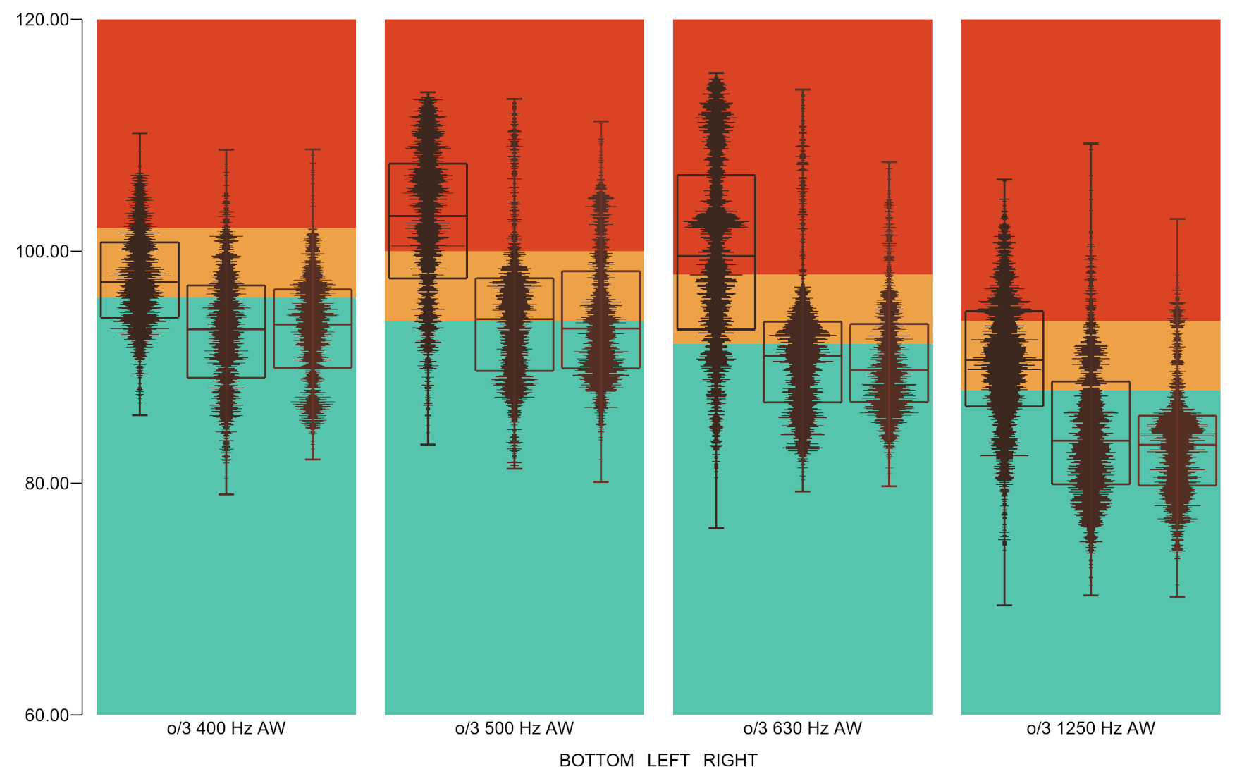


A series of boxplots with integrated histograms provide a better overview of the frequencies distributions across the cells, and still scales well with the number of cells. In contrast to the drill-down-view, which uses color encoding of the velocity level values, the boxplots uses positional encoding. Fig. 3(a) shows boxplots with a mirrored histogram for each of the frequency bands of interest. The background stripes show the limits, so that engineers can see how many cells belong to each level. In order to not loose the spatial context we suggest to split the plots according to the engine parts (Fig. 3(b)).
4.3 Detailed analysis across both domains
As soon as potentially problematic design parts are prioritized for a detailed examination, additional perspectives and interactions become necessary (requirements R3, R3a, and R3b). We need to show the velocity levels for all selected cells and for all harmonics that belong to the selected frequency band (R3a). To maintain a consistent coding, we apply the same color scheme as for the intermediate level, but additional visualization space is needed to account for the usually large number of cells. Since showing all harmonics is not an option, we decided to show all harmonics that belong to a selected frequency band (1 to 69 harmonics per frequency band). We dedicate one vertical bar to each harmonic and color it according to the area-normalized values of the discrete velocity levels. We place these bars right next to each other to optimize the use of the available visualization space. This provides a good way to compare multiple harmonics to each other.
To support all relevant analysis tasks, the view provides two sorting strategies: If each column is sorted independently, a quick overview of the area size and the magnitude of the velocity levels is provided. In this case, the lines in one row can belong to different cells (Fig. 4(b)). If spatial coherence is required, the user can sort the entire view by one selected column. This way, the engineer sees which harmonics share similar characteristics (Fig. 4(a)).
To achieve a more detailed analysis in the spatial domain (R3b), we integrate a suitably adapted 3D geometry view. Consistently, we also use the same color coding in this view to show velocity levels. To compare velocity levels across several harmonics that belong to the same frequency band, a series of linked 3D views is used – changing the perspective in one view leads to an according change in all other views (Fig. 5). The 3D view is also important to judge radiation efficiency (T3c). Velocity levels are indicators of noise, but the same velocity level can cause different levels of noise. If an engine part swings without changing its volume at a certain velocity, the resulting noise will be low. If, however, a part changes its volume, the noise will be high. Engineers need to inspect these parts and, based on their knowledge and experience, they can judge which parts with high velocity levels are indeed critical. An animated 3D view showing exaggerated deformations helps to identify spots with high radiation efficiency (Fig. 6).


Furthermore, engineers need to detect hot-spots at the surface (T3d). For the color mapping we opted for diverging shades instead of sequential scales to let the user see more differences in the data and to emphasize the extremes. Engineers are also familiar with this kind of color mapping. Custom color scales proved to be very efficient to achieve this. We decided to use a non-linear color scale which compensates for the logarithmic effects in the data given in decibels. Fig. 9(c) shows this color mapping and how it supports the detection of hot-spots at 400 Hz.
As we need to provide a joint analysis of both frequencies and spatial locations (R3), we found linked views a suitable solution. As soon as the user selects a harmonic in the harmonics pane, the selection is also shown in the linked 3D view, and vice versa.
4.4 Interaction design

NVH data is multi-faceted and it is not feasible to show all data in one integrated visualization. Linked views with appropriate interaction mechanisms allow to integrate several perspectives in the analysis [11]. We therefore link all views so that all selections and changes in any one view immediately get reflected consistently in all other views. In the following, we discuss our interaction design, related this setup of linked views.
Starting from the overview, engineers need to drill down into prioritized frequency bands and engine parts. To aid the detailed data assessment, we automatically show the corresponding harmonic pane (Fig. 4) when the user hoovers the pointer over a rectangle in the overview. The user can also click on any field in the overview to “freeze” the selection.
To refine the selection, the user can interact with the frequency band details pane (Fig. 5(c)), showing the integrated velocity values for the selected frequency band in four bars. The scales are linear in area size, as surface areas are key to identifying critical places. The right-most bar shows the proportion of threshold areas, i.e., the discrete velocity level acceptance. It is a magnified version of a particular cell shown in Fig. 2(b). Clicking on any of the three parts refines the selection accordingly. The third bar provides access to a subset of cells with velocity levels that exceed a certain, user-defined threshold. The second bar shows the most critical cells using a relative, percentage-based threshold, while the left-most bar is showing all values, ranked by the velocities. As the layout is linear with respect to the cell areas, the corresponding decibel values spread out according to their distribution. Grid lines help with related the bars to their respective scales.
It is also important to let users select cells in the 3D views, for example, by clicking onto one or several of them. A particularly useful interaction is to enlarge the set of selected cells, including additional neighboring cells. We found it helpful to also provide a growing mode that only includes additional cells if they exceed a certain velocity level. This way, even larger areas of relevant values can be easily selected in the 3D view (Fig. 7). Of course, standard interactions like zoom and rotation are also supported. Importantly, the 3D views can also be linked to always show the same perspective, regardless which of the views the user is interacting with.
We integrate the overview matrix pane, the harmonics pane, and the frequency band details pane into a single drill-down view with three panes. These visualizations are always used and represent the central point in the exploration process. After several iterations in our collaborative design process, we arrived at the decision to keep this view – the drill-down view – as a stable component in the top-left of the visualization at all time points. The drill-down view is integrated with additional coordinated views, including and adapted boxplots and geometry views. Fig. 5 shows a typical configuration from one of our evaluation sessions with 3D views showing the selected frequency band and three most critical harmonics right next to the drill-down view, as well as the adapted boxplot view underneath.
5 Use Case
To evaluate our approach, we engaged with a case study of data from a multi-body dynamics (MBD) simulation of a front-wheel drive (FWD) demo model at an operation point of 2000 RPM using AVL EXCITE™, a tool for advanced durability and NVH analysis. The model covers an inline four-cylinder (I4) internal combustion engine, a manual-transmission gearbox, the final drive/differential, and front axle shafts with brake flanges. The model is set to the 3rd gear. Three mechanical engineers who also coauthor the paper conducted the evaluation. Below, we describe the data first, followed by the evaluation.
5.1 Simulation data


Simulation and data recovery result in kinematic quantities (for displacement, velocity, and acceleration) in the time domain for the surface of the model. Nodal kinematic data is calculated in the frequency domain from which the average normal-to-surface velocity of each outer cell is obtained. The velocities are normalized to a reference area of 1 m2 and expressed in dB using AVL’s standard reference value.
In this case study, the outer surface has 13 047 vertices and 12 173 cell faces and it is partitioned into engine sides FRONT, REAR, TOP, BOTTOM, LEFT, and RIGHT (Fig. 8). Integrating the cell faces’ normal velocities across each surface partition area and/or each standard frequency band (octave, octave), we get the data as analyzed in this use case:
- •
For each cell face at the outer surface we get the sub-region it belongs to, its area, and the discrete velocity level in dB for each of 359 harmonics and 26 octaves.
- •
For each surface region we get its area and the integral velocity level for each harmonic and octave.
The simulation results are checked against two given criteria for velocity levels (both prescribed for octaves in the 215 Hz – 3150 Hz range at 2000 RPM):
- •
Integral velocity level limits in dB, applicable to levels obtained by integration of discrete levels across the whole outer surface of an engine.
- •
Discrete velocity level limits in dB, applicable to velocity levels calculated for the cells.


5.2 Overview first
The first task in the exploration process is gaining overview on parts and frequencies that are not conform to the prescribed limits (Fig. 2(a)). Using the overview matrix pane of the drill-down view, the overall engine “pass criteria” is checked. The yellowish rectangles in the TOTAL row for the 400, 500, 630 and 1250 Hz octaves indicate frequency bands where values are above a threshold.
A non-greenish color (yellowish or reddish) of rectangles related to sub-regions warns the analyst of high velocity levels in these sub-regions and within the corresponding frequency bands. It shows that these sub-regions – at these frequency bands – contribute the most to the engine’s overly high integral velocity levels. In the shown example, it is the BOTTOM region at the 500 and 630 Hz octave. The BOTTOM region contains the oil pan, a part of the engine which often requires a special attention during noise analysis.
Subsequently, the severity of the acceptance limits violation for the identified critical frequency bands at the engine level (represented by TOTAL region/row) is checked qualitatively by switching to our two-tone pseudo coloring mode (Fig. 10). This visualization mode shows how “deep” we are within the corresponding acceptance category (in our case: the yellowish ones).
5.3 Prioritize
Once the overview is gained, the experts prioritize the problematic parts in order to solve the biggest problems first. Comparing frequency bands with each other in Fig. 10, we also see relative violation severity, providing an importance order, in which the critical regions / frequency bands should be examined: in the 400 Hz octave we exceeded the acceptance limit just slightly (shades of green), in the 1250 Hz octave we entered more into the borderline area (shades of yellow), while in the 500 and 630 Hz octaves we are close to the unacceptable region (shades of red). So, the latter two frequency bands are examined first.


5.4 Detailed analysis
In order to quantify the limits violation, after qualitative exploration by means of visualization, we use tooltips (Fig. 11). By hovering the pointer over the drill-down’s top-left pane, we read just +0.1 dB and +1.3 dB over the acceptable limits for the 400 Hz and the 1250 Hz octaves, respectively, while we identify a quite significant excess of +5.4 dB and +5.7 dB in the 500 Hz and the 630 Hz octaves.
Switching off the limits/show option, we depict the calculated integral velocity level values. The highest integral velocity levels occur below 200 Hz: at the 67 Hz octave, followed by the 80 and 125 Hz octaves. This can also be seen for the discrete velocity levels as depicted in Fig. 2(f). These bands are outside the frequency range that is relevant for the noise analysis (the according limits are defined for the 215 Hz – 3150 Hz range) as the human ear is not that sensitive at lower frequencies (the identified high velocity levels could become a subject of the vibration analysis, though). Accordingly, the analysis focus remained on the “noise” frequency bands in which the integral velocity levels are found to exceed the acceptable limits: 400, 500, 630 and 1250 Hz.
The distribution of the discrete velocity levels (area-weighted) for a selection of frequency bands (octaves, octaves or harmonics) as well as of engine regions can be visualized using boxplots (Fig. 3(a)). The discrete velocity level distributions can be also shown against the discrete velocity level acceptance categories.
The matrix overview pane of the drill-down view (Fig. 2(d)) can also show how much area of each engine region satisfies discrete velocity level limits for each frequency band. From above we know that the integral velocity levels for the whole engine (TOTAL region) are the highest at the 400 Hz, 500 Hz, 630 Hz and 1250 Hz octaves. From the pane we see that the main contributors to these high values at the specified frequency bands are the velocity levels at the LEFT, RIGHT, and BOTTOM regions. As the heights of the rectangles are proportional to region areas, we see that among the three regions the most critical one is the BOTTOM region.
This information can also be seen in detail in the boxplots (Fig. 3(b)) using the split option that depicts the discrete velocity levels distributions for a selection of the critical engine regions / frequency bands, from left to right: BOTTOM, LEFT, RIGHT.
In addition to the qualitative information in the overview matrix pane of the drill-down view, we get also numerical values using the frequency band details pane (Fig. 5) by selecting the critical regions / frequency bands in the overview matrix pane. We read that for the BOTTOM region in the critical frequency bands 50 – 70 % of its area has discrete velocity levels above the acceptance level (yellowish or reddish).
To identify engine surface parts related to the critical regions / frequency bands spatially we use the 3D view. In addition to showing the discrete velocity level values (Fig. 9(b)), we can enable the limits flag to color the engine surface according to discrete acceptance criteria limits (Fig. 9(a)). Also, we can emphasize critical engine regions by showing the discrete velocity level values using a non-linear color distribution (Fig. 9(c)).
Supported by AVL IMPRESS™ 3D and AVL IMPRESS™/M, we can animate an exaggerated engine surface deformation for the targeted frequency bands. The surface is colored according to velocity levels in dB. This way, we can better focus on the identified acoustic hot spots and examine their deformation character.
5.5 Findings
Our exemplary analysis lead to the following findings:
- 1.
High velocity levels in the BOTTOM region due to bending of the front, left, rear and bottom sides of the oil pan (Fig. 9(b)).
- 2.
High velocity levels in the LEFT and RIGHT regions due to lateral swinging of the intake and exhaust manifolds (Fig. 12(a)).
- 3.
BOTTOM as the most critical engine region at the 630 Hz octave with monopole noise sources at the side walls of the oil pan, having high radiation efficiency (Fig. 12(b)).
- 4.
A vibration of the oil pan at the 1250 Hz octave shows an excitation of its higher modes, with less radiation efficiency (Fig. 12(c)).
- 5.
The intake and exhaust manifolds at all critical frequencies behave as so-called dipole noise sources, meaning their swinging has also a lower radiation efficiency (Fig. 12(a)).
As a result, in the next design iteration, we would focus on a reduction of oil pan velocity levels at the 500 and 630 Hz octaves by optimizing either the geometric design or its excitation.
6 Discussion
Designing an interactive visualization solution for domain experts poses several challenges. Commonly, automotive engineers have decades of experience in simulation, using certain forms of visualization on a daily basis. Usually, those amount to static images, which they use to make design decisions. In NVH studies, the data is large and multi-faceted, addressing spectral and spatial aspects, posing significant challenges for the analysis. The important semantic structures of both the frequency and the spatial domain imply additional challenges.
Analyzing such data at multiple levels of detail is tedious with standard tools. Still, it is essential to flexibly relate frequencies and spatial locations for a successful analysis. Our solution provides an integrated approach to jointly studying spatial and frequency aspects, from the overview level to a detailed analysis. This amounts to a major improvement over the state of the art. Many additional details, like custom color scales, synced 3D views, easy cells selections, ranking based brushing, etc., further improve the impact of the new approach.
The participatory design and development process, from the first exchange between simulation and visualization to the eventually designed visualization tool, was long and required numerous discussions, clarifications, many versions of design, including multiple different color scales, etc. Looking back, we realize how important it was to repeatedly discuss visual analytics principles with the domain experts.
Due to the limited time the experts could spend for the evaluation and the fact that the data has to be pre-processed for the prototype, our solution was so far only used for the data presented in the use case in Section 5. The overall feedback for the final prototype was very positive. Earlier, the domain experts had to use several tools for the analysis. They had to identify a problematic point in the Campbell diagram, then load corresponding results in a charting tool, look at the velocity charts per cell for a certain frequency, and finally highlight the cell in the 3D result viewer. The new ease of accessing details and identifying spatial locations of the problematic cells is a very appreciated feature. Their feedback on our integrated solution was very positive since it enables them to quickly browse through the whole data while keeping the context and not needing to switch applications. We did not formally measure the speed-up, but engineers stated that the new approach is much faster. One consequence of the speed-up is that they can check much more details now. They can now very easily get data for a certain harmonic or a frequency band and hence check much more data which is not located at problematic points. This helps in getting insight and a better comprehension of the data. Finally, the experts also stressed how the feature-rich interactive approach helps them in understanding the complexities of the analyzed system, and makes the identification of problematic spots easier in both domains. They stated that they cannot wait to have the new approach, including the data pre-processing, implemented in their production software, so that more data sets could be explored. They gladly demonstrated the prototype to other colleges in their department to gain support for the integration into the production software. Thanks to the positive feedback from these demonstrations the process of integration has started.
The new approach was used repeatedly to confirm what the domain experts knew from experience already. Still, often the only way of communicating their findings is through standardized reports. To ensure that such reports are accepted by their customers and that they can be compared with other reports, standard color scales and charts must be used. Changing well-established domain conventions takes long time, if it happens at all. We hope that the integration in the production software will aid this process among NVH engineers.
It is often desirable to semantically aggregate data and to use a hierarchical approach to exploration. Frequency bands are a standard way of doing aggregation of harmonics in acoustics, but other domains often have similar concepts. Some of our solutions also could be used in other domains with similar types of spectral data.
Spectral imaging is often used in medicine and geology. In both domains, the spatial component is also very important. If both spatial and frequency components are present, it is necessary to provide simultaneous access to and visualization of both components. Furthermore, some of our visual encoding solutions, such as splitting of heatmap cells to show overview and detail or using a two-tone coloring inspired approach to depicting values in heatmaps, can be used in many application domains.
7 Conclusion
We present results of a collaboration between NVH domain experts and visualization researchers, i.e., a novel visual analysis solution for noise simulation data. Our approach enables a quick drill-down from octave frequency bands to the individual harmonics without loosing the overview of the hierarchical data structure. The exploratory data analysis takes place simultaneously in the frequency and spatial components views. We see the potential that other professionals, who are concerned with multi-faceted data including frequency and spatial aspects, can draw valuable inspiration from our here presented solution.
Future directions of our research include the extension of the proposed approach to ensemble simulations and its evaluation in the context of different simulation models. The internal combustion engine was selected here since the domain experts are familiar with it and it seemed the most appropriate choice for a use case. Including other views, and interactively analyzing the data in a more abstract manner, and by means of automatic analysis methods, also, represent another important avenue for future research. We plan to explore novel use cases from different application domains with similar data.
Acknowledgements
VRVis is funded by BMK, BMDW, Styria, SFG, Tyrol and Vienna Business Agency in the scope of COMET (879730) which is managed by FFG. Parts of this work have been done in the context of CEDAS, i.e., the Center of Data Science at the University of Bergen, Norway. Parts of this work have been supported by Virginia Tech Institute for Creativity, Arts, and Technology.
References
- [1] M. P. Boyce. Rotor dynamics. In M. P. Boyce, ed., Gas Turbine Engineering Handbook, chap. 5, pp. 215–250. Butterworth-Heinemann, Waltham, MA 02451, fourth ed., 2012.
- [2] W. Campbell. The protection of steam turbine disk wheels from axial vibration. In Proceedings of the Spring meeting of the American Society of Mechanical Engineers, 1924.
- [3] F. Di Marco, R. D’Amico, and F. Ronzio. Electric motor encapsulation design for improved NVH: a CAE-based approach. In Proceedings of the INTER-NOISE and NOISE-CON Congress and Conference, number 7, pp. 2464–2474, 2019.
- [4] H. Doleisch, M. Gasser, and H. Hauser. Interactive feature specification for focus+context visualization of complex simulation data. In Proceedings of the Eurographics / IEEE VGTC Symposium on Visualization, pp. 239–248, 2003. doi: 10.2312/VisSym/VisSym03/239-248
- [5] X. Dominguez, P. Arboleya, P. Mantilla-Perez, I. El-Sayed, N. Gimenez, and M. A. DiazMillan. Visual analytics-based computational tool for electrical distribution systems of vehicles. In Proceedings of the 2019 IEEE Vehicle Power and Propulsion Conference, VPPC, pp. 1–5, Oct. 2019. doi: 10.1109/VPPC46532.2019.8952440
- [6] J. Eirich, J. Bonart, D. Jäckle, M. Sedlmair, U. Schmid, K. Fischbach, T. Schreck, and J. Bernard. IRVINE: A design study on analyzing correlation patterns of electrical engines. IEEE Transactions on Visualization and Computer Graphics, 2021. doi: 10.1109/TVCG.2021.3114797
- [7] J. Eirich, D. Jäckle, T. Schreck, J. Bonart, O. Posegga, and K. Fischbach. VIMA: Modeling and visualization of high dimensional machine sensor data leveraging multiple sources of domain knowledge. In Proceedings of the 2020 Visualization in Data Science, VDS, pp. 22–31, Oct. 2020. doi: 10.1109/VDS51726.2020.00007
- [8] N. Hampl. Advanced simulation techniques in vehicle noise and vibration refinement. In X. Wang, ed., Vehicle Noise and Vibration Refinement, chap. 8, pp. 174–188. Woodhead Publishing, 2010. doi: 10.1533/9781845698041.2.174
- [9] M. Harrison. Vehicle Refinement: Controlling Noise and Vibration in Road Vehicles. Elsevier Butterworth-Heinemann, Burlington, MA, 2004.
- [10] J. Kehrer and H. Hauser. Visualization and visual analysis of multifaceted scientific data: A survey. IEEE Transactions on Visualization and Computer Graphics, 19(3):495–513, 2013. doi: 10.1109/TVCG.2012.110
- [11] D. Keim, G. Andrienko, J.-D. Fekete, C. Görg, J. Kohlhammer, and G. Melançon. Visual Analytics: Definition, Process, and Challenges, pp. 154–175. Springer, 2008. doi: 10.1007/978-3-540-70956-5_7
- [12] J. Kniss, G. Kindlmann, and C. Hansen. Interactive volume rendering using multi-dimensional transfer functions and direct manipulation widgets. In Proceedings of the 2001 IEEE Visualization Conference, IEEE VIS’01, pp. 255–262. IEEE, 21–26 Oct. 2001.
- [13] T. Langer and T. Meisen. Visual analytics for industrial sensor data analysis. In Proceedings of the 23rd International Conference on Enterprise Information Systems, ICEIS, pp. 584–593, 2021. doi: 10.5220/0010399705840593
- [14] D. Mandke, D. Ghaisas, S. Pawar, and S. Suh. Numerical prediction and verification of noise radiation characteristics of diesel engine block. In Proceedings of the Noise and Vibration Conference & Exhibition. SAE International, 2019. doi: 10.4271/2019-01-1591
- [15] A. Neeman, B. Jeremic, and A. Pang. Visualizing tensor fields in geomechanics. In Proceedings of the 2005 IEEE Visualization Conference, IEEE VIS’05, pp. 35–42. IEEE, 23–28 Oct. 2005.
- [16] J. Prajith and V. Sagade. NVH full vehicle development – virtual simulation process for low frequency structure-borne regions. In Proceedings of the WCX SAE World Congress Experience. SAE International, 2020. doi: 10.4271/2020-01-1266
- [17] J. C. Roberts. State of the art: Coordinated & multiple views in exploratory visualization. In Proceedings of the Fifth International Conference on Coordinated and Multiple Views in Exploratory Visualization, CMV 2007, pp. 61–71, 2007. doi: 10.1109/CMV.2007.20
- [18] T. Saito, H. Miyamura, M. Yamamoto, H. Saito, Y. Hoshiya, and T. Kaseda. Two-tone pseudo coloring: Compact visualization for one-dimensional data. In Proceedings of the 2005 IEEE Symposium on Information Visualization, INFOVIS 2005, pp. 173–180. IEEE, 23–25 Oct. 2005.
- [19] T. Saito, H. N. Miyamura, M. Yamamoto, H. Saito, Y. Hoshiya, and T. Kaseda. Two-tone pseudo coloring: compact visualization for one-dimensional data. In Proceedings of the IEEE Symposium on Information Visualization, INFOVIS, pp. 173–180, 2005. doi: 10.1109/INFVIS.2005.1532144
- [20] M. Sedlmair, P. Isenberg, D. Baur, M. Mauerer, C. Pigorsch, and A. Butz. Cardiogram: Visual analytics for automotive engineers. In Proceedings of the SIGCHI Conference on Human Factors in Computing Systems, pp. 1727–1736. Association for Computing Machinery, 2011. doi: 10.1145/1978942.1979194
- [21] A. B. Shaik Mohammad, R. Vijayakumar, and N. R. Panduranga. Structure borne noise optimization of diesel engine by simulation. In Proceedings of the International Conference on Advances in Design, Materials, Manufacturing and Surface Engineering for Mobility. SAE International, 2017. doi: 10.4271/2017-28-1944
- [22] A. B. Shaik Mohammad, R. Vijayakumar, and N. R. Panduranga. Vibro-acoustic optimization of 3 cylinder diesel engine components for lower sound radiation using finite element techniques. In Proceedings of the Symposium on International Automotive Technology. SAE International, 2019. doi: 10.4271/2019-26-0189
- [23] B. Shneiderman. The eyes have it: A task by data type taxonomy for information visualizations. In Proceedings 1996 IEEE Symposium on Visual Languages, pp. 336–343. IEEE, 3–6 Sept. 1996.
- [24] V. Souksavanh and Y. Liu. NVH data analytics and its application in vehicle rating. In Proceedings of the 2020 IEEE 7th International Conference on Industrial Engineering and Applications, ICIEA, pp. 287–292. IEEE, 2020. doi: 10.1109/ICIEA49774.2020.9101968
- [25] J. A. Stevens. Visualization of complex automotive data: A tutorial. IEEE Computer Graphics and Applications, 27(6):80–86, 2007. doi: 10.1109/MCG.2007.161
- [26] J. W. Tukey et al. Exploratory data analysis, vol. 2. Reading, MA, 1977.
- [27] D. Vernon-Bido, A. Collins, and J. Sokolowski. Effective visualization in modeling & simulation. In Proceedings of the 48th Annual Simulation Symposium, pp. 33–40. Society for Computer Simulation International, San Diego, 2015.
- [28] X. Wang. Rationale and history of vehicle noise and vibration refinement. In X. Wang, ed., Vehicle Noise and Vibration Refinement, chap. 1, pp. 3–17. Woodhead Publishing, 2010. doi: 10.1533/9781845698041.1.3
- [29] X. Zheng and A. Pang. Volume deformation for tensor visualization. In Proceedings of the 2002 IEEE Visualization Conference, IEEE VIS’02, pp. 379–386. IEEE, 27 Oct.–1 Nov. 2002.