Mie Scattering with 3D Angular Spectrum MethodJournal: oePublication type: Research Article

Let the global Cartesian base-vectors be ($\mathbf{e}_{x},\mathbf{e}_{y},\mathbf{e}_{z}$) in space $\mathbb{R}^{3}$, where position vector is $\mathbf{r}=x\mathbf{e}_{x}+y\mathbf{e}_{y}+z\mathbf{e}_{z}$ and global coordinates are marked as $r_{\text{glob}}=(x,y,z)$. Consider a generalized, compact surface $\Omega$ in $\mathbb{R}^{3}$, which has a continuously differentiable parametrization with parameters $p$ and $q$ as

Let us place the origin of the local coordinate system at point $\mathbf{o}(p,q$) on the surface $\Omega$, where two base vectors $\mathbf{f}_{1}$ and $\mathbf{f}_{2}$ define tangential plane at the point, and the third base vector $\mathbf{f}_{3}$ is a local surface normal vector, see Figure (1). When normalized, these vectors form an orthonormal base ($\mathbf{f}_{1},\mathbf{f}_{2},\mathbf{f}_{3}$) and are defined as

The final local base ($\mathbf{e}_{1},\mathbf{e}_{2},\mathbf{e}_{3}$) is obtained from the base ($\mathbf{f}_{1},\mathbf{f}_{2},\mathbf{f}_{3}$), when the local polarization of the electric field is chosen. Let us set

where the sign is chosen according to the desired electromagnetic propagation direction. In a simple case, when polarization is known on the surface $\Omega$, the local electric field vector $\mathbf{e}_{1}$ on $\Omega$ can be presented with the base ($\mathbf{f}_{1},\mathbf{f}_{2}$), and the local magnetic field vector $\mathbf{e}_{2}$ is obtained as a cross-product with local propagation direction $\mathbf{e}_{3}$ as $\mathbf{e}_{2}=\mathbf{e}_{3}\times\mathbf{e}_{1}$.

Polarization on the surface $\Omega$ can also have externally sourced initial conditions, for example, from a polarization of an incident beam, that creates the electric field distribution on the surface $\Omega$. Let $\mathbf{p}=\mathbf{p}(p,q)$ be a vector that is perpendicular to the plane of that incident beam polarization. Then, local direction $\mathbf{e}_{1}$ is an intersection of that plane, and the tangential plane of surface $\Omega$ spanned by ($\mathbf{f}_{1},\mathbf{f}_{2}$).

Thus $\mathbf{e}_{1}$, the base vector along the local electric field, and $\mathbf{e}_{2}$, the base vector along the local magnetic field, are obtained as

The vectors $(\mathbf{e}_{1},\mathbf{e}_{2},\mathbf{e}_{3}$ form a right-handed orthonormal base, which together with the origin $\mathbf{o}$ defines a local coordinate system. Let a vector $\mathbf{r}$ be presented in this base as $\mathbf{r}=\bar{x}\mathbf{e}_{1}+\bar{y}\mathbf{e}_{2}+\bar{z}\mathbf{e}_{3}$. Its coordinate triple is marked briefly as $r_{\text{loc}}=(\bar{x},\bar{y},\bar{z})$. When the vector $\mathbf{r}$ is expressed with both $(\mathbf{e}_{x},\mathbf{e}_{y},\mathbf{e}_{z}$) and $(\mathbf{e}_{1},\mathbf{e}_{2},\mathbf{e}_{3}$) bases, as it is known, the dependence of the coordinates on each other is determined by an orthogonal transformation matrix

where the columns are the coordinate triples $\mathbf{e}_{1,{\text{glob}}},\mathbf{e}_{2,{\text{glob}}}$ and $\mathbf{e}_{3,{\text{glob}}}$. Let the position $P$ be presented in global coordinate system as $\mathbf{r}=x\mathbf{e}_{x}+y\mathbf{e}_{y}+z\mathbf{e}_{z}$. Position $P$ presented in the local coordinate system with a global base is

Let´s denote briefly $\mathbf{\bar{r}}=\mathbf{r}-\mathbf{o}$. Thus, we have presentations of the location $\mathbf{\bar{r}}$ in both local and global coordinate systems. The dependence of the corresponding coordinates can be written using the transformation matrix Eq. (5) as

Let us divide the segment of the surface $\Omega$ containing the electric field distribution $E_{0}(p,q)$ into a finite partition of small separate sets $\cup_{c}\Omega_{c}=\Omega$. Select the point $\mathbf{o}(p,q$) on differential element $\Omega_{c}$, the vectors associated with it are $\mathbf{e}_{1}$ and $\mathbf{e}_{2}$. Area $\Omega_{c}$ is projected to the plane spanned by the vectors $\mathbf{e}_{1}$ and $\mathbf{e}_{2}$. The resulting area at the plane is marked as $\Omega_{t}$. Likewise, function $E_{0}$ is projected into that plane, limited to set $\Omega_{t}$ and zero elsewhere. This geometry is presented in Figure 2. The resulting projection is marked as $E_{0}^{t}$. In the local coordinate system it holds $\bar{z}=0$ on the piece $\Omega_{t}$, because this is located on the $\bar{x}\bar{y}-$plane. $E_{0}^{t}$ is valid when $\bar{x}\approx 0$ and $\bar{y}\approx 0$.

The angular spectrum theory is locally applied on the local coordinate system to function $E_{0}^{t}$ valid on piece $\Omega_{t}$. Let’s observe the field it creates at point $\mathbf{\bar{r}}$, where the coordinates are as in Eq. (6). At a fixed point $\mathbf{r}$ holds [19]

where $\mathcal{F}\big\{E_{0}^{t}\big\}$ is the Fourier transform of the local electric field $E_{0}^{t}$ and $k=(k_{x}^{2}+k_{y}^{2}+k_{z}^{2})^{1/2}$ is the wavenumber. The total field from the arbitrary surface is obtained by summing the fields from the differential sources by the superposition principle as

where local coordinates $(\bar{x},\bar{y},\bar{z})$ as in Eq. (6) and the total field is polarized along the global $\mathbf{e}_{1}$ unit-vector. The obtained field Eq. (9) also satisfies the Helmholtz equation as unit vector $\mathbf{e}_{1}$ is locally constant. To be precise, if the limit with respect to the areas $|\Omega_{t}|$ of the sets $\Omega_{t}$ exists, we define

As pointed out at the beginning of the Theory section, this limit also works physically when considering smooth surfaces and is even more precise when the wavelength decreases compared to the local radius of the surface. Finally, a further examination is made to obtain a closed form for clause Eq. (10); we present a proof in Appendix A.

Heuristically, when $|\Omega_{t}|$ shrinks, the function $E_{0}^{t}/[E_{0}^{t}(\bar{0},\bar{0})|\Omega_{t}|]$, normed in volume, approaches a Dirac delta $\delta_{(0,0)}$ in the sense of the distribution theory; $E_{0}^{t}/[E_{0}^{t}(\bar{0},\bar{0})|\Omega_{t}|]\rightarrow\delta_{(0,0)}$ thus $E_{0}^{t}\rightarrow E_{0}^{t}(\bar{0},\bar{0})|\Omega_{t}|\delta_{(0,0)}$. As known, the Fourier transform of Dirac delta is 1, thus, by small $|\Omega_{t}|$

since $E_{1}(p,q)=E_{1}^{t}(\bar{0},\bar{0})$ when $\mathbf{o}$ is fixed. Then Eq. (9) and Eq. (11) yield first the form of a Riemann sum and then an integral as a limit

The final form can be written as

where

and $\bar{x},\bar{y}$ and $\bar{z}$ are as in Eq. (6) and notation $(\mathbf{r};p,q)$ defines electric field on observation point $\mathbf{r}$ related to the location ($p,q)$ on the parametrizied surface. Propagating waves are obtained by integrating Eq. (14) over the real disk $k_{\bar{x}}^{2}+k_{\bar{y}}^{2}\leq k^{2}$, and evanescence waves can be obtained by expanding the integration over the real domain, i.e., $k_{\bar{x}}^{2}+k_{\bar{y}}^{2}>k^{2}$.

There are two key observations regarding this derivation. First, Eq. (14) is similar to $\mathbf{E}_{t}=-\nabla\times(\mathbf{M}G)$ after replacing the scalar Green’s function ($G$) by its angular spectrum given by Weyl identity, where $\mathbf{M}=-2\mathbf{n}\times\mathbf{e}_{2}$ is a small magnetic dipole [26]. Thus, Eq. (13) is a particular case of the Stratton-Chu equation for the electric field in which only the magnetic sources $\mathbf{M}=-\mathbf{n}\times\mathbf{E}_{surf}$ are presented and the electric ones $\mathbf{J}=\mathbf{n}\times\mathbf{H}_{surf}$ have been removed [27]. Secondly, if the surface $\Omega$ is planar, Eq. (13) and Eq. (14) return to the original two-dimensional angular spectrum method.

An electromagnetic beam in the plane wave spectrum representation also has polarization vector components along the propagation direction. To account for polarization let us expand Eq. (14) along plane $(\mathbf{e}_{1},\mathbf{e}_{3})$ using the relation $\mathbf{E}_{t}\cdot\mathbf{k}=0$ [28]. Let $\mathbf{k}=k_{\bar{x}}+k_{\bar{y}}+k_{\bar{z}}$ be the wave vector, where $k=\|\mathbf{k}\|$ is the wave number and $k_{z}=[k^{2}-k_{\bar{x}}^{2}-k_{\bar{y}}^{2}]^{1/2}$. Moreover let´s denote $\mathbf{s}=\frac{1}{k}\mathbf{k}$ and define $\mathbf{r}_{||}=\bar{x}\mathbf{e}_{1}+\bar{y}\mathbf{e}_{2}+|\bar{z}|\mathbf{e}_{3}$. Hence the summarized exponent in Eq. (14) can be written as $i(k_{\bar{x}}\bar{x}+k_{\bar{y}}\bar{y}+k_{\bar{z}}|\bar{z}|)=i\mathbf{k}\cdot\mathbf{r}_{||}=ik(\mathbf{s}\cdot\mathbf{r}_{||})$, obtaining

where $\mathbf{e}_{0}(k_{\bar{x}},k_{\bar{y}},k_{\bar{z}})$ defines the polarization. The local Cartesian coordinate system presents differential source Eq. (15) in the base $(\mathbf{e}_{1},\mathbf{e}_{2},\mathbf{e}_{3}$). When expanded to the VSH presentation, the influence of each differential source must be presented by means of position vector $\mathbf{r}$ to preserve the spherical symmetry of VSH. Next, the global mapping of local coordinates is presented.

We have a simple connection $(\mathbf{r}-\mathbf{o})_{\text{glob}}=\Theta\,\mathbf{\bar{r}}_{\text{loc}}$ as in Eq. (6). Let us define $\mathbf{s}_{||}=\mathbf{s}$, when $\bar{z}>0$, but, when $\bar{z}<0$, the sign of $\bar{z}-$coordinates in $\mathbf{s}$ is exchanged. Consequently, we can write

where written briefly $\mathbf{t}=\mathbf{\bar{s}}_{{||},{loc}}$. As a result, we get

Based on Eq. (17), the term $e^{ik(\mathbf{s}\cdot\mathbf{\bar{r}}_{||})}$, which is in the local coordinate system, can be presented in the global coordinate system as

where $e^{-ik(\mathbf{t}\cdot\mathbf{o}_{\text{loc}})}=e^{-ik(\mathbf{s}_{||}\cdot\mathbf{o})}$ presents the position and phase shift of the source beam’s focus (waist) from global origin to the source surface. Each local beam created from the differential source is presented in a global coordinate system.

Modified BSCs coefficients for each source point are derived for presenting any parameterized field distribution in a global coordinate system, including the locations and orientations of the sources. These coefficients map complicated coordinate geometries into one presentation. This allows synthesizing a total electromagnetic beam as a superposition of VSH expanded fields.

The integration wave numbers $k_{\bar{x}},k_{\bar{y}}$ in Eq. (15) are analogous to the BSC angles [20]. Thus Eq. (15) is expressed in the direction cosine coordinate system as

where $\xi$ and $\zeta$ are direction cosines related to Cartesian coordinates as $k\cos{\xi}=k_{\bar{x}}$ and $k\cos{\zeta}=k_{\bar{y}}$. The polarization $\mathbf{e}_{0}$ in terms of direction cosines is given as

and the vector $\mathbf{s}$ is

Then, Eq. (19) is evaluated by numerical integration over a disk of radius $k$ using the trapezoidal rule method, which is sufficiently accurate for periodic functions [29], with uniform-width $l$ [20]

where indices $i$ and $j$ refer to individual plane waves with propagation constants $k_{\bar{x}}^{i}$ and $k_{\bar{y}}^{j}$ respectively to $\bar{x}$ and $\bar{y}$ directions, and $p=\xi_{t+1}-\xi_{t}=\zeta_{t+1}-\zeta_{t}$ is the step size of the numerical integration and $\mathbf{t}_{ij}=(\mathbf{s}_{{||},{ij}})_{\text{loc}}$. The integration radius is limited to $k\leq 2\pi/\lambda$ for obtaining only propagating waves, and the evanescence fields can be obtained by expanding the integration domain.

The transformation matrix from local coordinates ($\bar{x},\bar{y},\bar{z}$) to global coordinates ($x,y,z$) is $\Theta(p,q)$ as in Eq. (5), and the radiated electric field can be written at an arbitrary point $\mathbf{r}$ by VSHs as [20]

where $\mathbf{M}^{1}_{\text{emn}},\mathbf{M}^{1}_{\text{omn}},\mathbf{N}^{1}_{\text{emn}}$ and $\mathbf{N}^{1}_{\text{omn}}$ are the VSH of the first kind and $D_{mn}$ is a normalization factor [20]. For $k\mathbf{r}$ we have to substitute its spherical coordinates $(kr,\theta,\phi)$ and corresponding spherical base vectors $(\mathbf{e}_{\theta},\mathbf{e}_{\phi})$, taken with respect to the local base $(\mathbf{e}_{1},\mathbf{e}_{2},\mathbf{e}_{3})$. They can be computed from the triple $r_{\text{loc}}$. Modified BSCs $a^{t}_{\text{emn}},a^{t}_{\text{omn}},b^{t}_{\text{emn}}$ and $b^{t}_{\text{omn}}$ are given as

The BSCs for each $ij-$ plane wave $a^{t}_{{\text{emn}}_{ij}},a^{t}_{{\text{omn}}_{ij}},b^{t}_{{\text{emn}}_{ij}}$ and $b^{t}_{{\text{omn}}_{ij}}$ are defined in Appendix B. Now the magnetic field is obtained by rearranging the modified BSCs and by multiplying by constant $-i/\eta$ as

The total incident electric field Eq. (13) and total incident magnetic field from the source distribution, accounting for polarization as in Eq. (15), is written as the integration of vector spherical harmonics expansions Eq. (23) and Eq. (25) over the source surface as

Similar scattered field presentations mapped with the T-matrix method are presented as

where $\mathbf{E}_{scat}$ and $\mathbf{H}_{scat}$ are introduced in Appendix B.

In summary, we have expanded planar 2D ASM to 3D ASM by dividing the surface into infinitesimally small sub-regions used as local source points. We mapped source points’ global location and orientation information into the modified BSCs and obtained the total fields as a superposition of VSH-expanded source points. Also, surface polarization can be modified by parameterization.

The total field from arbitrary surface $\Omega$ is obtained as a superposition of differential source fields $\mathbf{E}_{tot}=\sum_{\Omega}\mathbf{E}_{t}$. As shown in derivation, when the surface area of the differential source plane approaches zero, the result Eq. (14) is analagous to the angular spectrum presentation of a curl of the magnetic dipole multiplied with scalar Green’s function $\mathbf{E}_{t}=-\nabla\times(-2\mathbf{n}\times\mathbf{e}_{2}G)$. As is well known, the fields created in this way are exact from an infinitely large plane, and the method accurately approximates field synthesis from curved surfaces when the RoC is above a wavelength.

The radiation pattern of a differential source $\mathbf{E}_{t}$ is presented, where the magnetic dipole is positioned to the origin along the y-axis. Radiated fields are computed at transverse xy-plane and yz-plane; see Figure (3). This arrangement’s main polarization is along the x-axis, and the field propagates to the positive z-direction.

Figure (4) presents the radiated fields from a differential source on xy- and yz-planes.

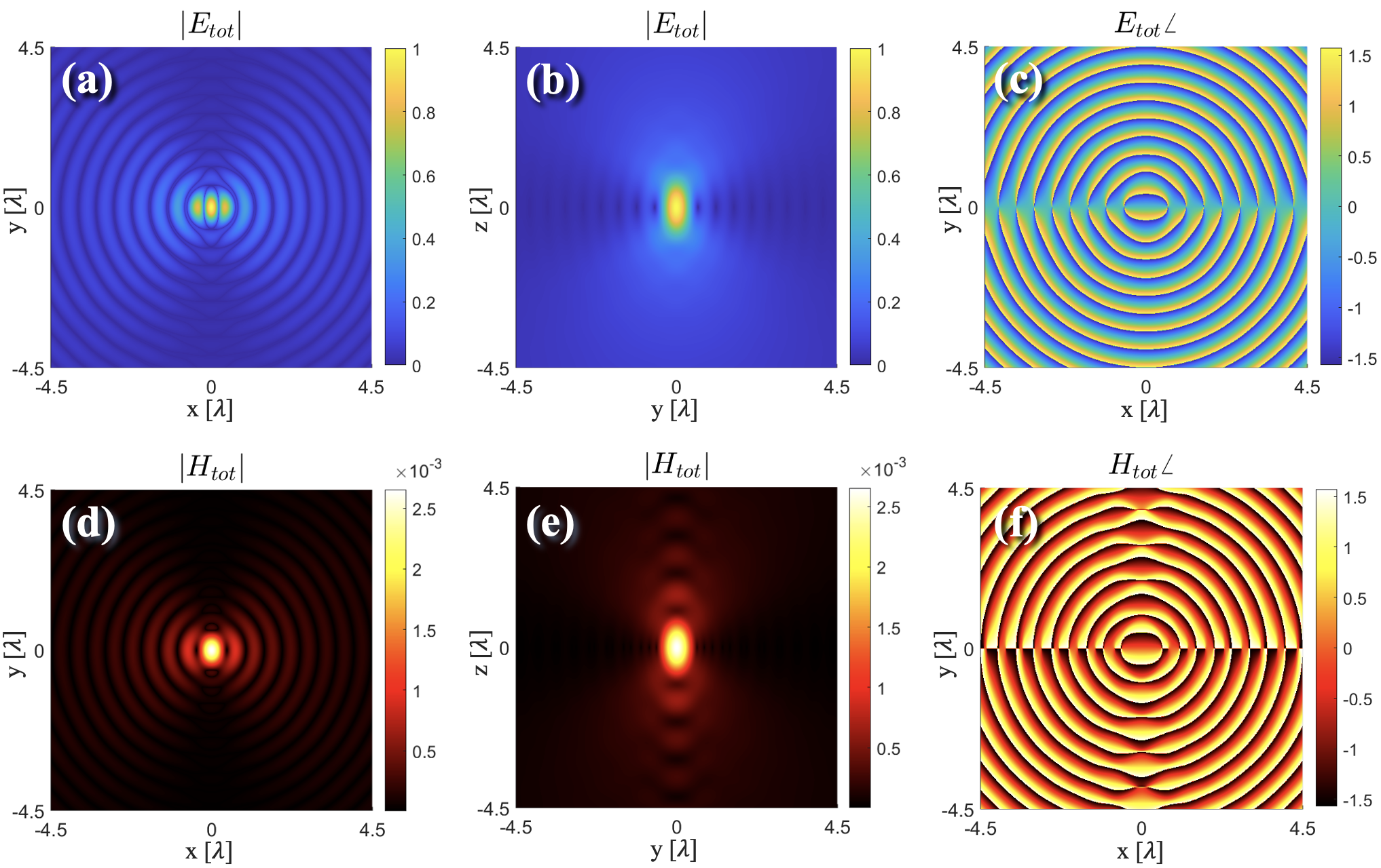
Simulation shows the free placement of source points inside the computation domain due to the absence of singularities. The maximum amplitude of the electric fields is one without normalization.

Mie scattering region is known for frequency-dependent backscatter intensity. This phenomenon is due to the scattering resonances, which trap energy temporally inside the sphere. Backscatter intensity is presented as a function of size parameter $k\alpha$, where $\k{=}k_{0}n$ is a refractive index dependent wavenumber inside the sphere and $\alpha$ is the radius of the sphere. These backscatter resonances are called morphology-dependent resonances (MDRs) [30, 31]. MDRs are highly responsive to simulation errors and are a good test of the accuracy of the derived 3D ASM combined with VSH expansion [32].

High accuracy manifests with simulations, where a Gaussian beam is created from its beam waist and its field components on a plane outside the beam waist. In the latter case, each source point has varying propagation direction and complex amplitude, making field synthesis on this computation inefficient with traditional methods. MDRs are computed with both source plane locations when the beam waist is positioned at the origin of the homogeneous sphere and on the side of the coated sphere, defined precisely later. Likewise, MDRs from an individual source point are computed in both focus scenarios, see Figure (5).

Simulations are executed by illuminating homogeneous and coated spheres by Gaussian beam in size parameter range $k\alpha\in[32,36]$ with beam waist radius $\omega_{0}=1.5\lambda$. Homogeneous spheres have a refractive index of $n_{r}=1.36$, and coated spheres have a $n_{r}=1.36$ core with a $n_{c}=1.5$ shell with radius of $0.7\ \alpha$. These values were selected from article [28] for comparing results. In both scenarios, the Gaussian beam is first synthesized on the transverse Plane 1 at the beam waist from the planar Gaussian electric field distribution with the traditional 2D AS and the proposed 3D AS method with an exact match. Then the incident field is computed on Plane 2 at $-5\ \alpha$ distance from the origin.

The second simulation synthesizes the same Gaussian beam from Plane 2 with the 3D ASM using equal $\lambda/6$ sampling space in the horizontal and vertical directions. Now each source point has locally varying propagation direction obtained as a Poynting vector $\mathbf{P_{inc}}=0.5\Re\big\{\mathbf{E_{inc}}\times\mathbf{H^{*}_{inc}}\big\}$ from the incident field synthesized from the Plane 1. Also, each source point is multiplied by the local complex electric field $\mathbf{E_{inc}}$ obtained from the first simulation, see simulation flow with source Planes 1 and 2 in Figure (6).

The Cartesian electric and magnetic field components of the incident field at Plane 2 are presented in Figure (7). These components are synthesized from Plane 1. Gaussian beam MDRs synthesized from both source plane scenarios are computed at -500 $\alpha$ distance from the origin [20] and compared in Figure (8). The resonances are labeled as $TE_{n,l}$ or $TM_{n,l}$, where $n$ indicates the mode number, and $l$ the number of radial peaks in the angle-averaged internal energy density distribution [20].

First, the homogeneous sphere is illuminated with a Gaussian beam focused at the origin. Second, a coated sphere is illuminated with a Gaussian beam focused on the side of the coated sphere $y=\alpha$ to verify even more specific resonance behavior. Also, the MDRs from a source point on Plane 2 in both scenarios are presented to underline the resonance difference with varying beam shapes.

Electromagnetic backscatter intensities show excellent MDRs matching from both source plane synthesis scenarios. The resonance shape, location, and peak spacing in Figure 8 match with values from [28]. In Figure (8 a), the peaks correspond to modes $TE_{39,1},TE_{40,1}$, and $TE_{41,1}$ respectively, and the spacing between the peaks satisfies the $\Delta k\alpha=\pi/2m_{r}\approx 1.15$ condition. Also, in Figure (8 b), the MDRs peaks from coated sphere correspond to the modes $TM_{39,1},TM_{40,1},TM_{41,1}$ and $TM_{42,1}$ respectively.

The MDRs of an individual differential source do not match the Gaussian beam resonances. However, a total beam created as a superposition of the differential sources from the surface $\Omega$ synthesizes the original beam with highly matching MDRs. This leads to the conclusion that the presented 3D AS method combined with the VSH expansion synthesizes electromagnetic scattering from multilayered spheres with high accuracy.

An elliptical surface was used as an example of a source distribution to synthesize a focused linearly polarized incident field using $\lambda/6$ sampling, see Figure (9). The incident field is compared to the Physical optics simulations at the yz-plane with an excellent agreement to less than a -39 dB difference in amplitude and less than the 0.1-degree difference in phase. Also, the scattered fields are computed from a $\alpha=$ 7.8 mm radius sphere in xz-plane with 100 dielectric layers with linearly varying permittivity $\epsilon_{r}\in[1-i0.001,\ 3-i0.01]$ from the surface to the center.

Base vectors for elliptical surfaces are derived from the Eq. (1 - 4) with the parametrization

with axial scaling factors $a_{x}=0.6,\ b_{y}=1.5,\ c_{z}=0.8$ and an unscaled radius $r=3$. The origin of the ellipsoid is shift $(x_{0},y_{0},z_{0})=(3,0,-0.5)$ compared to the sphere.

Figure (10) illustrate the amplitude and phase of the total field $\mathbf{E}_{tot}=\mathbf{E}_{inc}+\mathbf{E}_{scat}$ on xz-plane where $x,z\in[-5a,5a]$. Simulations are performed with $500\times 500$ evaluation points with size parameter of $k\alpha=13$ and VSH modes of $N=50$.

References

- [1] E. L. Roetman, R. P. Kochhar, and G. L. Hower, “An integral representation for the fields in electromagnetic scattering problems,” Electromagnetics 12, 1–15 (1992).
- [2] M. Gharghi, H. Bai, G. Stevens, and S. Sivoththaman, “Modeling and simulation of spherical solar cells,” in Conference Record of the Thirty-first IEEE Photovoltaic Specialists Conference, 2005., (2005), pp. 1177–1180.
- [3] N. Keerativoranan, P. Hanpinitsak, K. Saito, and J. I. Tadaka, “Circular mesh based physical optics for scattered field prediction,” IEEE Antennas and Wireless Propagation Letters pp. 1–1 (2021).
- [4] J. R. Sanford, “Scattering by spherically stratified microwave lens antennas,” IEEE Transactions on Antennas and Propagation 42, 690–698 (1994).
- [5] A. A. R. Neves and C. L. Cesar, “Analytical calculation of optical forces on spherical particles in optical tweezers: tutorial,” J. Opt. Soc. Am. B 36, 1525–1537 (2019).
- [6] G. Gouesbet, J. Lock, and G. Gréhan, “Generalized lorenz–mie theories and description of electromagnetic arbitrary shaped beams: Localized approximations and localized beam models, a review,” Journal of Quantitative Spectroscopy and Radiative Transfer 112, 1–27 (2011).
- [7] G. Gouesbet, “A scientific story of generalized lorenz–mie theories with epistemological remarks,” Journal of Quantitative Spectroscopy and Radiative Transfer 126, 7–15 (2013). Lasers and interactions with particles 2012.
- [8] Z. S. Wu, L. X. Guo, K. F. Ren, G. Gouesbet, and G. Gréhan, “Improved algorithm for electromagnetic scattering of plane waves and shaped beams by multilayered spheres,” Appl. Opt. 36, 5188–5198 (1997).
- [9] C. Bohren and D. R. Huffman, Absorption and Scattering of Light by Small Particles (Wiley Science Paperback Series, 1998).
- [10] G. Gouesbet, G. Gréhan, and B. Maheu, “Localized interpretation to compute all the coefficients gnm in the generalized lorenz–mie theory,” J. Opt. Soc. Am. A 7, 998–1007 (1990).
- [11] F. Onofri, G. Gréhan, and G. Gouesbet, “Electromagnetic scattering from a multilayered sphere located in an arbitrary beam,” Appl. Opt. 34, 7113–7124 (1995).
- [12] L. Mees, K. F. Ren, G. Gréhan, and G. Gouesbet, “Scattering of a gaussian beam by an infinite cylinder with arbitrary location and arbitrary orientation: numerical results,” Appl. Opt. 38, 1867–1876 (1999).
- [13] B. Maheu, G. Gouesbet, and G. Grehan, “A concise presentation of the generalized lorenz-mie theory for arbitrary location of the scatterer in an arbitrary incident profile,” Journal of Optics 19, 59–67 (1988).
- [14] J. A. Lock, “Partial-wave expansions of angular spectra of plane waves,” J. Opt. Soc. Am. A 23, 2803–2809 (2006).
- [15] A. V. Zvyagin and K. Goto, “Mie scattering of evanescent waves by a dielectric sphere: comparison of multipole expansion and group-theory methods,” J. Opt. Soc. Am. A 15, 3003–3008 (1998).
- [16] J. M. Taylor and G. D. Love, “Multipole expansion of bessel and gaussian beams for mie scattering calculations,” J. Opt. Soc. Am. A 26, 278–282 (2009).
- [17] G. Gouesbet, L. A. Ambrosio, and J. A. Lock, “On an infinite number of quadratures to evaluate beam shape coefficients in generalized lorenz-mie theory and the extended boundary condition method for structured em beams,” Journal of Quantitative Spectroscopy and Radiative Transfer 242, 106779 (2020).
- [18] J. Lamberg, F. Zarrinkhat, A. Tamminen, E. E. M. Khaled, and Z. Taylor, “Investigation of radial top-hat electric field distributions for corneal reflectometry using modified fourier optics method,” in 2021 46th International Conference on Infrared, Millimeter and Terahertz Waves (IRMMW-THz), (2021), pp. 1–2.
- [19] J. W. Goodman, Introduction to Fourier optics (Englewood, CO: Roberts, 2005).
- [20] E. E. M. Khaled, S. C. Hill, and P. W. Barber, “Scattered and internal intensity of a sphere illuminated with a gaussian beam,” IEEE Transactions on Antennas and Propagation 41, 295–303 (1993).
- [21] C.-Y. Hwang, S. Oh, I.-K. Jeong, and H. Kim, “Stepwise angular spectrum method for curved surface diffraction,” Opt. Express 22, 12659–12667 (2014).
- [22] L. Ebers, M. Hammer, and J. Förstner, “Light diffraction in slab waveguide lenses simulated with the stepwise angular spectrum method,” Opt. Express 28, 36361–36379 (2020).
- [23] N. G. Worku, R. Hambach, and H. Gross, “Decomposition of a field with smooth wavefront into a set of gaussian beams with non-zero curvatures,” J. Opt. Soc. Am. A 35, 1091–1102 (2018).
- [24] J.-S. Lee, T.-L. Song, J.-K. Du, and J.-G. Yook, “Near-field to far-field transformation based on stratton-chu fomula for emc measurements,” in 2013 IEEE Antennas and Propagation Society International Symposium (APSURSI), (2013), pp. 606–607.
- [25] A. Mazzinghi and A. Freni, “Analytical evaluation of the power radiated by sources arbitrarily distributed on a surface,” IEEE Transactions on Antennas and Propagation pp. 1–1 (2022).
- [26] W. C. Chew, Planarly Layered Media (1995), pp. 45–160.
- [27] W. Hsu and R. Barakat, “Stratton–chu vectorial diffraction of electromagnetic fields by apertures with application to small-fresnel-number systems,” J. Opt. Soc. Am. A 11, 623–629 (1994).
- [28] E. E. M. Khaled, S. C. Hill, and P. W. Barber, “Light scattering by a coated sphere illuminated with a gaussian beam,” Appl. Opt. 33, 3308–3314 (1994).
- [29] L. N. Trefethen and J. A. C. Weideman, “The exponentially convergent trapezoidal rule,” SIAM Review 56, 385–458 (2014).
- [30] B. R. Johnson, “Theory of morphology-dependent resonances: shape resonances and width formulas,” J. Opt. Soc. Am. A 10, 343–352 (1993).
- [31] D. Q. Chowdhury, S. C. Hill, and P. W. Barber, “Morphology-dependent resonances in radially inhomogeneous spheres,” J. Opt. Soc. Am. A 8, 1702–1705 (1991).
- [32] J. A. Lock, “Excitation efficiency of a morphology-dependent resonance by a focused gaussian beam,” J. Opt. Soc. Am. A 15, 2986–2994 (1998).
- [33] P. W. Barber and S. C. Hill, Light Scattering By Particles: Computational Methods (Advanced Series in Applied Physics, 1990).
- [34] U. P. O. Peña, “Scattering of electromagnetic radiation by a multilayered sphere,” IEEE Antennas and Propagation Magazine 57, 69–116 (2015).