Max Menssen
Department of Biostatistics
Leibniz Universität Hannover
Herrenäuser Straße 2
30419 Hannover
August 11, 2026
Abstract
A prediction interval is a statistical interval that should encompass one (or more) future observation(s) with a given coverage probability and is usually computed based on historical control data. The application of prediction intervals is discussed in many fields of research, such as toxicology, pre-clinical statistics, engineering, assay validation or for the assessment of replication studies. Anyhow, the prediction intervals implemented in predint descent from previous work that was done in the context of toxicology and pre-clinical applications. Hence the implemented methodology reflects the data structures that are common in these fields of research. In toxicology the historical data is often comprised of dichotomous or counted endpoints. Hence it seems natural to model these kind of data based on the binomial or the Poisson distribution. Anyhow, the historical control data is usually comprised of several studies. These clustering gives rise to possible overdispersion which has to be reflected for interval calculation. In pre-clinical statistics, the endpoints are often assumed to be normal distributed, but usually are not independent from each other due to the experimental design (cross-classified and/or hierarchical structures). These dependencies can be modeled based on linear random effects models. Hence, predint provides functions for the calculation of prediction intervals and one-sided bounds for overdispersed binomial data, for overdispersed Poisson data and for data that is modeled by linear random effects models.
Keywords
Bio-assay, historical control data, bootstrap calibration, assay validation and qualification
1 Introduction
A prediction interval is a statistical interval that should encompass future observations simultaniously with coverage probability
Similarly, lower prediction bounds should result in the coverage probability
and upper prediction bounds should have a coverage probability of
The computation of prediction intervals or bounds is based on the assumption that
both, the historicalobservations as well as the future observations
descent from the same data generating process.
The application of the prediction intervals implemented in predint
is of use in several fields of research, such as the detection of anti-drug antibodies
[Hoffmann and Berger 2011, Menssen and Schaarschmidt 2021] or
the validation of an actual control group by historical control data in toxicology
[Menssen and Schaarschmidt 2019]. Further applications of prediction intervals
can be found in industry [Ryan 2007], in experiments for method
comparison (bridging) or assay validation [Francq et al. 2019] or in the context of
the evaluation of replication studies [Spence and Stanley 2016].
All the applications mentioned above have in common, that the historical data used
for the calculation of prediction intervals is comprised of several clusters, rather
than of one unstructured sample.
For example, in pre-clinical experiments for the detection of anti-drug antibodies, it is of
interest to distinguish between ’responders’ whose anti-drug antibody reaction
exceeds a critical level and ’non-responders’ whose reaction is uncritical low.
One approach for the detection of such a critical level is the application of
an upper prediction bound that is calculated based on the observed anti-drug
antibody reaction of a set of known ’non-responders’.
Such experiments are usually run based on blood samples obtained from different
patients (or animals) and might be analysed
by different experimentors in different laboratories [Hoffmann and Berger 2011].
Since the experimental design is not of interest for answering the scientific question,
but reflects dependencies between experimental units (e.g. the samples that were
analysed in the same laboratory are not independent from each other due to
systematic error), random effects models have to be applied for modelling
and interval calculation.
The prediction intervals implemented in predint, that are based on random
effects models, are similar to the methodology proposed in Menssen and Schaarschmidt 2021.
But, additionally to the historical experimental design, two of the three implementations are
also able to take the design of the future data into account, rather than only the
number of future observations as proposed in Menssen and Schaarschmidt 2021.
Furthermore, the implemented methodology is applicable to a broad range of experimental
designs such as cross-classified and/or hierachical structures as well as balanced or
unbalanced data (see section 2.1).
Another example where clustered data occurs are bio-assays with a toxicological
background. These experiments are usually comprised of an untreated control group
that is compared to several groups of model organisms treated with a chemical
compound of interest.
In that field of research prediction intervals are of interest in order to validate
the outcome of an actual (or future) control group. Hence, such intervals are
calculated based on observations obtained from historical control groups of
previous experiments [Menssen and Schaarschmidt 2019, Valverde-Garcia et al. 2018].
Since many endpoints in toxicology are either dichotomous (e.g. rats with a tumor
vs. rats without a tumor) or counted observations (e.g. numbers of eggs per hen),
it seems natural to model them based on the binomial or the Poisson distribution,
respectively.
Anyhow, the model has to take the clustering into acount and hence also
possible overdispersion, meaning that the variance of the data exceeds the variance
that can be modeled based on ’simple’ binomial or Poisson distribution. One reason
for the presence of overdispersion are positive correleations between experimental units
in each cluster. Therefore, overdispersion is considered to be almost always present
in biological data [Demetrio et al. 2014, McCullagh and Nelder 1989].
Prediction intervals for future observation based on overdispersed binomial data
were proposed in Menssen and Schaarschmidt 2019. Anyhow, the prediction intervals
for that type of data that are implemented in predint are based on a slightly
different approach, meaning that they are also applicable in the case where
a simultainious prediction interval that should cover future observations
is needed (see section 2.2).
To the authors knowledge, prediction intervals for future observations
that can be computed based on clustered count data that exhibits ovsrdispersion were
not available in an R package hosted on CRAN. This gab is filled by
the prediction interval proposed in section 2.3.
2 Theory
2.1 Linear random effects models
A general linear random effects model is given by
where is a vector of random variables representing observations. The overall mean is represented by . is a stacked vector consisting of random effects sub-vectors . Hence, each represents all levels associated with a particular random factor out of the random factors that influence the observations. is a design matrix of dimensions where denotes the total length of . The random errors associated with the observations are represented by . The individual random effects can be represented as such that
with each
All random effects are assumed to be normal distributed as well as the errors . Furthermore it is assumed that
This model implies that the observations follow a multivariate normal distribution
| (1) |
with variance-covariance matrix
It is assumed that both, the historical as well as the future random variables are independent from each other, but descent from the same data generating process. Hence, also the future random variable that represents future observations is multivariate normal
| (2) |
with variance-covariance matrix
Please note, that the number of random effects per random factor might differ
between the historical and the future data (e.g. 5 hospitals, each with 3 patients
vs. 3 hospitals, each with 4 patients). Consequently, the number of observations
might differ between the historical and the future data ( is of
length and is of length ) as well as the variance-covariance
matrices and , since they depend on different
effects design matrices and .
This implies that, and usually do not follow the
same multivariate normal distribution (see eq. 1 and 2),
but, nevertheless, descent from the same data generating process which depends
only on the mean and the variance components .
In this setup, the error margin of the prediction is
with
which, in the case of a prediction for only future observation simplifies to
If a prediction interval for future observations should be computed based on observed historical data and the fitted model
the estimated prediction variance becomes
with as a square matrix with all entries set to one.
A prediction interval that should cover future observations
simultaniosly with coverage probability is given by
| (3) |
with as the -quantile of the multivariate t-distribution. Please note, that a prediction interval for future observation simplifies to
| (4) |
Menssen and Schaarschmidt 2021 gave an overview about several methods for the
computation of the prediction intervals given in equations 3 and 4
of which their bootstrap calibrated prediction interval serves as the basis of the intervals
implemented in predint.
2.2 Overdispersed binomial data
In several bio-assays run in the field of toxicology, the endpoints are dichotomous (e.g. rats with tumors vs. rats without tumors). A natural approach for modeling such data is the binomial assumption
| (5) | |||
with . In this notation is the binomial proportion,
is the size of clusters (e.g. number of individuals in the
th historical control group) and are the number of successes obtained from the
individuals of the th cluster (e.g. rats with tumors).
Anyhow, most of the biological data that is assumed to be binomial has higher
variability than expected and hence exhibits overdispersion [Demetrio et al. 2014, McCullagh and Nelder 1989].
There are two approaches to model overdispersion: The quasi-binomial (or quasi-likelihood)
approach or modelling based on the beta-binomial distribution.
The first approach assumes a dispersion parameter that constantly inflates the variance
for all observations, such that
with and .
For the latter, the data is assumed to be beta-binomial distributed
| (6) |
with , and . It is noteworthy,
that depends on the cluster size and becomes a constant,
if all of the clusters have the same size . In this case the
quasi-likelihood approach and the model that is based on the beta-binomial distribution
both result in overdispersion that constantly inflates the binomial variance
of the different clusters.
Several methods for the calculation of prediction intervals based on one binomial
sample were proposed in literature [Hahn et al. 2017]. Anyhow,
none of these methods reflect the fact that the historical data is usually comprised of several
clusters. Furthermore, these methods do not consider for possible overdispersion
and hence, yield coverage probabilities far below the nominal level, if overdispersion
is present in the data [Menssen and Schaarschmidt 2019].
The prediction intervals for dichotomous data that are implemented in predint
are derived from an asymptotic prediction interval for future observation,
which is based on one unclustered binomial sample [Hahn et al. 2017].
Its calculation is based on the assumption that
approximately follows a standard normal distribution
In this notation is the expected future observation, is the future random variable, is the estimate for the binomial proportion obtained from the historical sample of size and is the size of the future cluster. The corresponding prediction interval for future observation is given by
| (7) |
with and .
As mentioned above, this interval was proposed for the application to one historical
set of unclustered observations. Therefore, this prediction interval does not
account for clustering and hence, neglects the possible effect of overdispersion
that might occur in the data.
Prediction intervals for future observation, that account for the clustered
structure of the historical data, can be calculated based on both, the quasi-binomial
approach or the beta-binomial distribution.
A prediction interval that is based on the quasi-binomial assumption
can be obtained by substituting with and with in eq. 7. Hence, the interval is defined as
| (8) |
with .
A prediction interval for one future observation that is based on the beta-binomial distribution is computed if is substituted by and by in eq. 7. The resulting prediction interval is given as
| (9) |
Please note, that prediction intervals that should cover future observations simultainiously, can be obtained by the application of the bootstrap-calibration procedure described below in section 2.4.
2.3 Overdispersed Poisson data
In several bio-assays, such as avian reproduction, the variable of interest is comprised of count data [Valverde-Garcia et al. 2018]. A natural approach for modeling counts is to assume them to be Poisson distributed
Here, are the observations per cluster, is the index for the clusters and is the Poisson mean. Similar to dichotomous data, overdispersion is usually present and can be modeled based on the quasi-Poisson (quasi-likelihood) approach that grounds on a constant dispersion parameter inflating the Poisson-variance [Demetrio et al. 2014], such that
with and . Another approach for modeling overdispersed Poisson data is the negative-binomial distribution where the means of the historical studies follow a gamma distribution with parameters and , such that
with and [Gsteiger et al. 2013]. Please note that in the case in which several counted observations simply vary around their expected value , both, the quasi-Poisson and the negative-binomial assumption are not in contradiction with each other (with regard to their variance formula). This is because both, and are constant in this case. Hence,
| (10) |
Several methods for the calculation of prediction intervals for one future observation based on one Poisson distributed historical sample are reviewed in [Hahn et al. 2017]. An asymptotic prediction interval for future observation which is based on one unclustered Poisson distributed sample is based on the assumption that
| (11) |
is approximately standard normal
The corresponding asymptotic prediction interval is given by
Please note that this interval is a simplified version (ignoring offsets) of the one that is reviewd in [Hahn et al. 2017]. Its adaption to overdispersed data comprised of clusters results in
| (12) |
with . Simultanious prediction intervals for future observations can be obtained by the application of the bootstrap calibration procedure described in the next section.
2.4 Bootstrap calibration
The bootstrap-calibration of statistical intervals dates back to the late 1980ies.
The original approach proposed by Loh 1987 was aimed to find a better value
for the with which an interval is calculated in order to bring the coverage
probability of the calibrated interval as close as possible to the nominal .
This approach is reviewed in Efron and Tibshirani 1994 and is sometimes called
alpha-calibration.
Contrary to alpha-calibration, the bootstrap-calibration procedure used for the
calculation of the prediction intervals implemented in predint, is aimed to
find a coefficient that directly replaces the t- or z-quantiles in
eq. 4, 8, 9 and
12 resulting in prediction intervals for future
observations
| (13) |
for which the coverage probability is as close as possible to the nominal level
| (14) |
In this notation, is the vector of the future
observations, is the estimate for the expected future observation and is the prediction error.
Please note, that all prediction intervals implemented in predint are of
the form given in eq. 13. For interval calculation, the estimates
that correspond to , and ,
which off cause depend on the chosen model, are simply plugged in. Bootstrap
calibrated prediction intervals can be obtained depending on the following algorithm:
- 1.
Fit a random effects model to the historical data set in order to obtain the estimates , and
- 2.
Draw parametric bootstrap samples that follow the same experimental design as the future data
- 3.
Additionally, draw further bootstrap samples that follow the same experimental design as the historical data.
- 4.
Fit the initial model to in order to obtain , and .
- 5.
Choose a start-value for .
- 6.
Calculate prediction intervals based on the bootstrapped estimates as
- 7.
Calculate the coverage probability for the prediction intervals that correspond to the particular as
(15) with if and if .
- 8.
Alternate and repeat step six and seven until is satisfactory close to the nominal . Use this particular value of for the calculation of the calibrated prediction interval.
- 9.
Calculate the calibrated prediction interval based on the chosen and the parameter estimates from the initial model as shown in equation 13.
Please note, that for all prediction intervals implemented in predint the search for in step 8 of the calibration algorithm depends on the following bisection:
- 1.
Define start values and such that the corresponding bootstrap coverage probabilities and estimated following eq. 15 are
- 2.
Start the first of bisection steps by defining
- 3.
Calculate the corresponding bootstrap coverage probability according to eq. 15
- 4.
If , calculate
If , calculate
- 5.
Calculate the bootstrap coverage probability according to eq. 15
- 6.
Repeat this iteration process until or a maximum number of bisection steps was done.
- 7.
Use this particular for the calculation of the calibrated interval (repalace by in eq. 13).
3 Methodology implemented in predint
3.1 Prediction intervals
Since all functions for the calculation of prediction intervals (see tab. 1) depend on the same calibration approach and the intervals are of the same form (see eq. 13), all functions share a common framework in terms of applicability. The arguments common to all functions for interval calculation are given in tab. 2.
| Function name | Functionality |
|---|---|
| lmer_pi_unstruc() | |
| lmer_pi_futvec() | PI based on random effects modeles |
| lmer_pi_futmat() | |
| beta_bin_pi() | PI for overdispersed binomial data |
| quasi_bin_pi() | |
| quasi_pois_pi() | PI for overdispersed count data |
| Argument | Functionality |
|---|---|
| alternative | Prediction intervals or bounds , |
| alpha | Definition of |
| nboot | Number of bootstrap samples |
| delta_min | Lower start value for bisection |
| delta_max | Upper start value for bisection |
| tolerance | Tolerance for bisection |
| traceplot | Graphical overview about the bisection |
| n_bisec | Max. number of bisection steps |
Prediction intervals are calculated with alternative="both", which is the
default setting. Anyhow, if lower prediction bounds are of interest, alternative
has to be set to "lower". Upper prediction bounds are computed with
alternative="upper". Please note, that bootstrap calibration of prediction
bounds is done by adopting eq. 15, where , if alternative
is set to "upper", or if alternative is set to "lower".
If not specified explicitely, all functions calculate prediction intervals (or bounds)
with coverage probability which can be alterated by setting alpha
to any value between 0 and 1.
The number of bootstrap samples can be specified by nboot wich is set to
10000 by default.
Start values for the bisection are provided by the arguments delta_min
and delta_max which are set to default values of 0.01 and 10. The maximum
number of bisection steps is controlled via n_bisec and is per default 30.
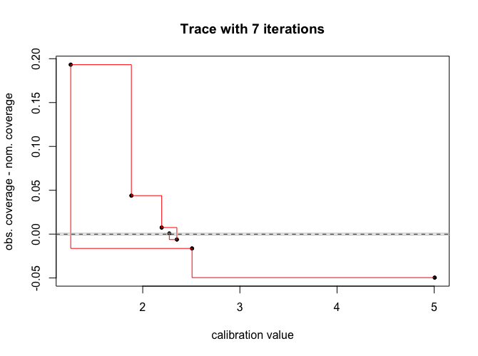
A graphical overview about the bisection process is given if traceplot=TRUE
(see fig. 1). In such a plot, the calibration values ,
calculated during the bisection, are given on the x-axis. The y-axix shows the
difference between the observed bootstrap coverage probabilities
and the nominal level . The bisection stops if or, if this is not the case, after the maximum number of steps defined
via n_bisec.
In rare occasions it might happen, that the estimated coverage probabilities
do not converge to the nominal level . This happens
if with controlled via
tolerance. In this case the value for from the last bisection step
is chosen for interval calculation in eq. 13. The user can
decide either to use the calculated interval or to change the search-interval
for by changing lambda_min and
lambda_max. Alternatively one might increase the tolerable level around the
nominal coverage probability via tolerance.
Please note, that due to the discretenes of dichotomous or count data, the true
coverage probability of the interval might not approach the desired in
some occasions. Consequently, also the bisection might not converge to the
nominal level. In such cases the calibrated prediction interval corresponding to
the last of the bisection steps, should be the one with coverage
probability closest to the nominal level.
3.1.1 Prediction intervals based on linear random effects models
Prediction intervals, that are based on random effects modeles fit with lme4::lmer() to the historical data, can be computed using lmer_pi_unstruc(), lmer_pi_futvec() or lmer_pi_futmat(). These intervals depend on the historical mean which is extracted from the fitted model with lme4::fixef(), its estimated variance drawn from the fitted model with lme4::vcov.merMod() and , the sum of the variance components extracted from the fitted model with lme4::VarCorr(). Substituting these estimates into eq. 13 results in a bootstrap calibrated prediction interval
| (16) |
This interval can be applied either in the case where a prediction for one future observation is needed,
as well as in the case where future observations should be predicted.
In the examples below, c2_dat1 will serve as an example for a
historical data set. It descents from a two way completely cross-classified design
with three replications per random factor and three replications per interaction
term and is therefore comprised of 27 observations.
R> c2_dat1

       y_ijk a b
1  105.27359 1 1
2  101.40640 1 1
3   94.01300 1 1
4   97.82988 2 1
5   94.30743 2 1
6   92.52234 2 1
7  102.17317 3 1
8   99.74908 3 1
9  100.64042 3 1
10  95.49433 1 2
11  92.30937 1 2
12  99.88281 1 2
13 103.82970 2 2
14  99.95517 2 2
15 107.13102 2 2
16 107.42282 3 2
17 105.25822 3 2
18 108.82881 3 2
19 107.30048 1 3
20 107.13083 1 3
21 106.73200 1 3
22 106.44846 2 3
23 104.60098 2 3
24 103.86882 2 3
25 107.01238 3 3
26 106.06968 3 3
27 107.53004 3 3
A random effects model that reflects the experimental design of c2_dat1, can be fitted with
R> # install.packages("lme4")
R> library(lme4)
R> fit <- lmer(y_ijk~(1|a)+(1|b)+(1|a:b), data=c2_dat1)
In all three functions, the fitted model has to be specified via model.
Please note, that at the current state, only models
in which the random effects are specified as (1|random effect) are
supported.
The bootstrap sampling of future observations is the same
in all three functions, if a prediction interval for future observation is
needed. This is because, internally, the future data is bootstrapped from the fitted model
via lme4::bootMer() of which one observation per bootstrap data set
is randomly chosen to serve as
in step 2 of the calibration process. Hence all three functions
yield the same prediction interval in this case.
R> set.seed(1234)
R> lmer_pi_unstruc(model=fit, m=1, alternative="both", nboot=10000)
  m hist_mean quant_calib pred_se  lower    upper
1 1  102.3971    2.273359 5.923724 88.93033 115.8638
R> set.seed(1234)
R> lmer_pi_futvec(model=fit, futvec=1, alternative="both", nboot=10000)
  m hist_mean quant_calib  pred_se    lower    upper
1 1  102.3971    2.273359 5.923724 88.93033 115.8638
R> set.seed(1234)
R> lmer_pi_futmat(model=fit, newdat=1, alternative="both", nboot=10000)
  m hist_mean quant_calib  pred_se    lower    upper
1 1  102.3971    2.273359 5.923724 88.93033 115.8638
The output of the three functions is a data.frame where m is the
number of future observations the prediction interval should cover (in this case one).
The historical mean is given by hist_mean and
quant_calib is the bootstrap calibrated coefficient used for the calculation
of the interval ( in eq. 13). pred_se is the
estimated standard error of the prediction (
in eq. 13) and lower and upper are the lower and
the upper bounds of the prediction interval.
The only difference between the three functions is the way how the bootstrap samples
are drwan, if a prediction interval for future observations
is needed. In the examples below, predint::c2_dat3 will serve as a future
data set that descents from the same data generating process, but has only two observations
per random factor and hence eight observations in total.
R> c2_dat3
      y_ijk a b
1  97.47232 1 1
2  95.44895 1 1
3 100.18817 2 1
4  99.36843 2 1
5  99.08363 1 2
6 101.11561 1 2
7  97.05361 2 2
8  97.81136 2 2
lmer_pi_unstruc() is a direct implementation of the prediction interval
described in Menssen and Schaarschmidt 2021. Hence, if the bootstrapped future
observations are sampled in two steps. Firstly, bootstrap samples
that have the same
experimental structure as the historical data are sampled using lme4::bootMer().
Then, observations are drawn randomly from the bootstrapped data in order to serve
as in the calibration. Therefore, only the number of future
observations, but not the experimental design of the future data set is
considered.
A prediction interval for future observations can be obtained, if m
is set to 8 or if the future data set c2_dat3 is directly specified
via newdat.
R> set.seed(1234)
R> lmer_pi_unstruc(model=fit, m=8, alternative="both", nboot=10000)
  m hist_mean quant_calib  pred_se    lower    upper
1 8  102.3971    3.366016 5.923724 82.45774 122.3364
R> set.seed(1234)
R> lmer_pi_unstruc(model=fit,
                   newdat=c2_dat3,
                   alternative="both",
                   nboot=10000)
      y_ijk a b hist_mean quant_calib  pred_se    lower    upper cover
1  97.47232 1 1  102.3971    3.366016 5.923724 82.45774 122.3364  TRUE
2  95.44895 1 1  102.3971    3.366016 5.923724 82.45774 122.3364  TRUE
3 100.18817 2 1  102.3971    3.366016 5.923724 82.45774 122.3364  TRUE
4  99.36843 2 1  102.3971    3.366016 5.923724 82.45774 122.3364  TRUE
5  99.08363 1 2  102.3971    3.366016 5.923724 82.45774 122.3364  TRUE
6 101.11561 1 2  102.3971    3.366016 5.923724 82.45774 122.3364  TRUE
7  97.05361 2 2  102.3971    3.366016 5.923724 82.45774 122.3364  TRUE
8  97.81136 2 2  102.3971    3.366016 5.923724 82.45774 122.3364  TRUE
If newdat is specified, the output is a data.frame in which the
first columns represent the data set specified via newdat.
hist_mean, quant_calib, pred_se, lower and upper are the same as
above. cover gives a statement whether the observation is covered
by the interval or not.
Contrary to lmer_pi_unstruc(), lmer_pi_futvec() accounts
for the experimental design of the future data and is applicable if the experimental
design of the future data is part of the design of the historical experiment(s).
If a prediction interval for
future observations is needed, a vector of row numbers that define the
experimental structure of the future data based on the historical data set has to be
specified.
R> futvec <- c(1, 2, 4, 5, 10, 11, 13, 14)
defines the rows in c2_dat1 that correspond to the experimental design of c2_dat3 (two observations per random factors a and b and their interaction). In other words, if the observations defined by the row numbers given in futvec are subsetted from c2_dat1, these subset will appear to descent from the same experimental design as c2_dat3.
R> c2_dat1[futvec, ]
       y_ijk a b
1  105.27359 1 1
2  101.40640 1 1
4   97.82988 2 1
5   94.30743 2 1
10  95.49433 1 2
11  92.30937 1 2
13 103.82970 2 2
14  99.95517 2 2
Internally, the bootstrap samples corresponding to the future observations are sampled with lme4::bootMer(). Then for each of the bootstrap samples, a subset that is comprised of the observations in the rows defined by futvec is drawn and serves as in the calibration. A prediction interval for the 8 future observations in c2_dat3 can be obtained with
R> set.seed(1234)
R> lmer_pi_futvec(model=fit, futvec=futvec, alternative="both", nboot=10000)
  m hist_mean quant_calib  pred_se    lower    upper
1 8  102.3971     3.30748 5.923724 82.80448 121.9897
If the future data should appear in the output, it can be specified via newdat but, of cause its data structure has to correspond to the structure defined by futvec.
R> set.seed(1234)
R> lmer_pi_futvec(model=fit,
               futvec=futvec,
               newdat=c2_dat3,
               alternative="both",
               nboot=10000)
      y_ijk a b hist_mean quant_calib  pred_se    lower    upper cover
1  97.47232 1 1  102.3971    3.287969 5.923724 82.92006 121.8741  TRUE
2  95.44895 1 1  102.3971    3.287969 5.923724 82.92006 121.8741  TRUE
3 100.18817 2 1  102.3971    3.287969 5.923724 82.92006 121.8741  TRUE
4  99.36843 2 1  102.3971    3.287969 5.923724 82.92006 121.8741  TRUE
5  99.08363 1 2  102.3971    3.287969 5.923724 82.92006 121.8741  TRUE
6 101.11561 1 2  102.3971    3.287969 5.923724 82.92006 121.8741  TRUE
7  97.05361 2 2  102.3971    3.287969 5.923724 82.92006 121.8741  TRUE
8  97.81136 2 2  102.3971    3.287969 5.923724 82.92006 121.8741  TRUE
Despite its user friendliness lmer_pi_futvec() has one drawback: It is only
applicable if the experimental design of the future data is included in the experimental
design of the historical data. In other words, lmer_pi_futvec() is not
applicable if the number of observations per random factor is bigger in the future
data than in the historical data (e.g. if data will be observed from four future
laboratories but the historical data contains only three historical ones).
This problem can be overcome by using lmer_pi_futmat(), which is the only
function in which the future observations are directly bootstraped from
the experimental design of the future data.
As already stated in section 2.1, a prediction intervall
for future observations depends on the numbers of observations per
random factor in the future data set. Hence, the variance-covariance matrices
and for the historical and the future observations
differ from each other if .
The bootstrap sampling used in lmer_pi_futmat() is based on the following
algorithm which is implemented in lmer_bs() (see section 3.2):
- 1.
Obtain the estimates for the mean and the variance components based on the model fit to the historical data set.
- 2.
Define the design matrices each of dimensions , with as the number of future observations and as the number of observations per random factor in the future data set.
- 3.
Draw random samples that correspond to the random effects, such that and .
- 4.
Calculate the bootstrap sample as .
- 5.
In order to obtain bootstrap samples, repeat step 1 to 4 for times.
If the future data is handed over via newdat, the bootstrap depends on a list containing the design matrices that was created using lme4::lFormula(). Hence each random factor in newdat needs at least two replications. A prediction interval for c2_dat3 is given with
R> set.seed(1234)
R> lmer_pi_futmat(model=fit,
               newdat=c2_dat3,
               alternative="both",
               nboot=10000)
      y_ijk a b hist_mean quant_calib  pred_se   lower    upper cover
1  97.47232 1 1  102.3971    3.326992 5.923724 82.6889 122.1053  TRUE
2  95.44895 1 1  102.3971    3.326992 5.923724 82.6889 122.1053  TRUE
3 100.18817 2 1  102.3971    3.326992 5.923724 82.6889 122.1053  TRUE
4  99.36843 2 1  102.3971    3.326992 5.923724 82.6889 122.1053  TRUE
5  99.08363 1 2  102.3971    3.326992 5.923724 82.6889 122.1053  TRUE
6 101.11561 1 2  102.3971    3.326992 5.923724 82.6889 122.1053  TRUE
7  97.05361 2 2  102.3971    3.326992 5.923724 82.6889 122.1053  TRUE
8  97.81136 2 2  102.3971    3.326992 5.923724 82.6889 122.1053  TRUE
Sometimes a random factor in the future data set might not have any replicate e.g. if the historical data descents from trials that were done in several different laboratories, but the experiments for the future observations were carried out in another one. This is the case in c2_dat4, where the factor b has only one observation.
R> c2_dat4
     y_ijk a b
1 102.8583 1 1
2 101.1324 1 1
3 104.9425 2 1
4 101.2299 2 1
5 104.6727 2 1
6 105.3402 2 1
Here, the future data can not be specified via newdat since lme4::lFormula() can not handle such cases. Alternatively, a list that contains the design matrices can be provided via futmat_list. Please note, that the order of the design matrices has to correspond to the order by which the random factors are handled in the initial model that was fit to the historical data with lme4::lmer(). A list of design matrices corresponding to c2_dat4 is given by
R> fml <- vector(length=4, "list")
R>
R> names(fml) <- c("a:b", "b", "a", "Residual")
R>
R> fml[["a:b"]] <- matrix(nrow=6, ncol=2,
                       data=c(1,1,0,0,0,0,
                              0,0,1,1,1,1))
R>
R> fml[["b"]] <- matrix(nrow=6, ncol=1,
                     data=c(1,1,1,1,1,1))
R>
R> fml[["a"]] <- matrix(nrow=6, ncol=2,
                     data=c(1,1,0,0,0,0,
                            0,0,1,1,1,1))
R>
R> fml[["Residual"]] <- diag(6)
R>
R> fml
$‘a:b‘
     [,1] [,2]
[1,]    1    0
[2,]    1    0
[3,]    0    1
[4,]    0    1
[5,]    0    1
[6,]    0    1


$b
     [,1]
[1,]    1
[2,]    1
[3,]    1
[4,]    1
[5,]    1
[6,]    1

$a
     [,1] [,2]
[1,]    1    0
[2,]    1    0
[3,]    0    1
[4,]    0    1
[5,]    0    1
[6,]    0    1

$Residual
     [,1] [,2] [,3] [,4] [,5] [,6]
[1,]    1    0    0    0    0    0
[2,]    0    1    0    0    0    0
[3,]    0    0    1    0    0    0
[4,]    0    0    0    1    0    0
[5,]    0    0    0    0    1    0
[6,]    0    0    0    0    0    1
The corresponding prediction interval is given by
R> set.seed(1234)
R> lmer_pi_futmat(model=fit,
                  futmat_list=fml,
                  alternative="both",
                  nboot=10000)
  m hist_mean quant_calib  pred_se    lower    upper
1 6  102.3971    3.034316 5.923724 84.42263 120.3715
3.1.2 Prediction intervals for overdispersed binomial data
Prediction intervals for overdispersed binomial data can be calculated based on the quasi-likelihood aproach using quasi_bin_pi() or based on the beta-binomial assumption using beta_bin_pi(). Because overdispersion appeals as a constant if the cluster size is the same, qb_dat1 will serve as an example for the historical data on which prediction intervals will be calculated based on both assumptions. The data set is comprised of the numbers of success (e.g. rats with tumors) vs. the number of failures (e.g. rats without a tumor) obtained in 10 clusters, each comprised of 50 experimental untits (e.g. rats).
R> qb_dat1
   succ fail
1     0   50
2     9   41
3    13   37
4     1   49
5     4   46
6     5   45
7    13   37
8     7   43
9     7   43
10    6   44
Based on the quasi-likelihood approach, quasi_bin_pi() calculates bootstrap calibrated prediction intervals for future numbers of success
with as the size of future clusters.
Please note, that the calculation of predciction intervals depend on the future
cluster size and hence, the calculated prediction intervals are different,
if the size of the future clusters differs beween each other.
The historical data set has to be specified histdat and needs to be a
data.frame with two columns, of which one describes the numbers of success
and the other the numbers of failures.
Then, internally, the estimation of and is done based on a
generalized linear model, fit with
glm(cbind(histdat[,1],histdat[,2]) ˜ 1, family=quasibinomial(), data=histdat).
The bootstrap data used in step two and three of the calibration process described
above, is sampled using the rqbinom() function which is described in detail
in section 3.2.
A prediction interval for the number of success in one future cluster of size 50
can be obtained with
R> set.seed(1234)
R> quasi_bin_pi(histdat=qb_dat1, newsize=50, nboot=10000)
  total hist_prob quant_calib  pred_se lower    upper
1    50      0.13   0.9855859 10.72381     0 17.06923
The resulting output is a data.frame in which total indicates the future
cluster size , hist_prob is the estimate for the historical binomial proportion
, quant_calib is the bootstrap calibrated coefficient used for
the calculation of the interval ( in eq. 13).
pred_se is the prediction error
and the prediction interval is given by lower and upper.
Prediction intervals that simultainiously cover future numbers of success
which are observed in clusters of size 40, 50 and 60 can be calculated with
R> set.seed(1234)
R> quasi_bin_pi(histdat=qb_dat1, newsize=c(40, 50, 60), nboot=10000)
  total hist_prob quant_calib  pred_se lower    upper
1    40      0.13    1.434355  8.75595     0 17.75915
2    50      0.13    1.434355 10.72381     0 21.88175
3    60      0.13    1.434355 12.68858     0 25.99993
If the future data should appear in the output, it can be specified via newdat. Please note, that the future data has to be of the same structure as the historical one (two variables, one for success and one for failures). Defining qb_dat2 via newdat results in the following output.
R> qb_dat2
  succ fail
1    0   40
2    6   44
3    8   52
R> set.seed(1234)
R> quasi_bin_pi(histdat=qb_dat1, newdat=qb_dat2, nboot=10000)
  succ fail total hist_prob quant_calib  pred_se lower    upper cover
1    0   40    40      0.13    1.434355  8.75595     0 17.75915  TRUE
2    6   44    50      0.13    1.434355 10.72381     0 21.88175  TRUE
3    8   52    60      0.13    1.434355 12.68858     0 25.99993  TRUE
In this output, three further variables occur: The first two variables are the
data set specified via newdat. total is the clustersite
and cover gives a statement, if the prediction intervals cover their
corresponding future observation (first column of the output).
Bootstrap calibrated prediction intervals that are based on the beta-binomial
assumption, can be computed with beta_bin_pi(). The resulting prediction
intervals are given as
Internally, the estimate of the binomial proportion is given as and the estimate for the intra-class correlation
is calculated following Lui et al. 2000.
The bootstrap calibration is done using the algorithm given in section 2.4,
with and sampled using rbbinom()
which is described in section 3.2. Please note,
that for the user, the functionallity of beta_bin_pi() is exactly the same
as of quasi_bin_pi(), meaning that the handling of historical and future
data does not differ from each other. Furthermore, the output of both functions
has the same format.
A prediction interval for the number of success in one future cluster of size 50
can be obtained with
R> set.seed(1234)
R> beta_bin_pi(histdat=qb_dat1, newsize=50, nboot=10000)
  total hist_prob quant_calib  pred_se lower    upper
1    50      0.13    2.429453 4.395622     0 17.17896
Simultanious prediction intervals for the numbers of success out of three clusters of size 40, 50 and 60 can be obtained by
R> set.seed(1234)
R> beta_bin_pi(histdat=qb_dat1, newsize=c(40, 50, 60), nboot=10000)
  total hist_prob quant_calib  pred_se lower    upper
1    40      0.13    3.405039 3.643114     0 17.60495
2    50      0.13    3.405039 4.395622     0 21.46727
3    60      0.13    3.405039 5.144237     0 25.31633
If a future data set (in this case predint::bb_dat2) is available, it can be specified via newdat
R> set.seed(1234)
R> beta_bin_pi(histdat=qb_dat1, newdat=bb_dat2, nboot=10000)
  succ fail total hist_prob quant_calib  pred_se lower    upper cover
1   11   29    40      0.13    3.405039 3.643114     0 17.60495  TRUE
2    1   49    50      0.13    3.405039 4.395622     0 21.46727  TRUE
3    3   57    60      0.13    3.405039 5.144237     0 25.31633  TRUE
3.1.3 Prediction intervals for overdispersed Poisson data
Bootstrap calibrated prediction intervals for overdispersed Poisson data are implemented in quasi_pois_pi() and are calculated as
| (17) |
with as the calibrated coefficient used in eq. 13. Please note, that the sampling of bootstrap data and in step two and three of the calibration process is done based on rqpois(), which will be described below in section 3.2. The data set qp_dat1 contains sampled data that mimics historical observations (e.g. eggs per hen over two years) obtained from several clusters (e.g. studies).
R> qp_dat1
[1] 46 62 30 59 74 53 32 27 59 47
A prediction interval for one future observation is given by
R> set.seed(1234)
R> quasi_pois_pi(histdat=data.frame(qp_dat1), m=1, nboot=10000)
  m hist_mean quant_calib  pred_se    lower    upper
1 1      48.9    2.253848 16.23642 12.30559 85.49441
Please note, that the historical data specified via histdat needs to be a data.frame. The number of future observations that should be covered by the prediction interval can be specified by m. A prediction interval for future observations can be obtained by
R> set.seed(1234)
R> quasi_pois_pi(histdat=data.frame(qp_dat1), m=3, nboot=10000)
  m hist_mean quant_calib  pred_se lower    upper
1 3      48.9    3.092852 16.23642     0 99.11683
If the future data is already available (here qp_dat2), it can be specified via newdat
R> qp_dat2
[1] 44 74 36
R> set.seed(1234)
R> quasi_pois_pi(histdat=data.frame(qp_dat1),
                 newdat=data.frame(qp_dat2),
                 nboot=10000)
  qp_dat2 hist_mean quant_calib  pred_se lower    upper cover
1      44      48.9    3.092852 16.23642     0 99.11683  TRUE
2      74      48.9    3.092852 16.23642     0 99.11683  TRUE
3      36      48.9    3.092852 16.23642     0 99.11683  TRUE
3.2 Functions for data sampling and bootstrapping
Since, all prediction intervals implemented in predint are based on bootstrap calibration, functions for the sampling of new observations from the models described above are necessary. An overview about these functions is given in table 3.
| Function name | Functionality |
|---|---|
| lmer_bs() | Bootstrapping from random effects models |
| rbbinom() | Sampling of beta-binomial data |
| rqbinom() | Sampling of quasi-binomial data |
| rqpois() | Sampling of quasi-Poisson data |
3.2.1 Bootstrapping from random effects models
In principle, bootstrapping from linear random effects models fit with lme4::lmer()
can be done with lme4::bootMer(). Anyhow, the bootstrap samples obtained
with lme4::bootMer() are bound to have the same experimental structure (same
numbers of observations per random factor) as the original data set the model was
fit to.
As already stated in section 2.1, a simultainious prediction intervall
for future observations depends on the numbers of observations per
random factor in the future data set. Hence, the variance-covariance matrices
and for the historical and the future observations
usually differ from each other.
A bootstrap function, that is able to sample new data sets based on the estimated
mean and variance components drawn from a random
effects model fit with lme4::lmer(), in which the bootstraped data does
not have to be of the same structure as the initial data, is provided via lmer_bs()
and is based on the sampling algorithm described in section 3.1.1.
lmer_bs() depends on the following arguments: model, newdat, futmat_list
and nboot.
model defines the random effects model fit with lme4::lmer(). Please
note, that lmer_bs() only works for models in which random effects are
specified as (1 | random effect).
nboot defines the number of bootstrap samples .
If newdat is defined, the design matrices are computed
using lme4::lFormula. But, as described before, lme4::lFormula requires
at least to observations per random factor. If this is not the case, a list containing the
design matrices can be supplied via futmat_list.
Based on the fitted model
R> fit <- lmer(y_ijk~(1|a)+(1|b)+(1|a:b), c2_dat1)
100 bootstrap samples that have the same experimental structure as c2_dat3 can be sampled with
R> lmer_bs(model=fit, newdat=c2_dat3, nboot=100)
Alternatively new data can be sampled based on a list that contains the design matrices that can be specified via futmatlist
R> lmer_bs(model=fit, futmat_list=fml, nboot=100)
with fml defined above in section 3.1.1.
3.2.2 Sampling of beta-binomial data
If the data is assumed to be beta-binomial distributed, such that
with clusters of size and intra-class correlation coefficinent
it can be sampled using the following mechanism:
Based on given values for and , the parameters of the beta-distribution
and can be calculated as
with . Then, the binomial proportions for each cluster are sampled from the beta distribution
and the numbers of successes for each cluster are sampled to be
for a given cluster size .
Please note, that this sampling mechanism only works if is bigger than zero
but smaller than one.
This approach is implemented in rbbinom() in which n refferes to
the number of clusters , size refferes to the cluster
size , prob referes to the expected binomial proportion and
rho to the intra class correlation coefficient .
A data set with ten clusters, each comprized of 50 experimental units, an expected
success probability of 0.1 and an intra class correlation of 0.06 can be sampled
as
R> rbbinom(n=10, size=50, prob=0.1, rho=0.06)
3.2.3 Sampling of quasi-binomial data
Quasi-binomial data sampling is based on the assumption that the binomial variance is inflated by a dispersion paramter that is constant for all clusters
This type of data can be sampled from the beta-binomial distribution using the
following mechanism:
For a given cluster size and a given dispersion parameter ,
the sum of the parameters of the beta-distribution differs between the
clusters and is given by
| (18) |
Subsequently, and can be calculated individually for each cluster, based on a predifined value between 0 and 1 for
Then, the binomial proportions for each cluster are sampled from individual beta distributions
and the numbers of succes for each cluster are sampled to be
Please note, that this sampling mechanism works only, if and
. Both, a dispersion parameter of as well as
result in negative in eq. 18 and hence in negative
values for and as well. Furthermore, and
result in . Anyhow, the beta-distribution is only defined if their
parameters are positive numbers greater than zero.
An implementation of this sampling process is provided via rqbinom() wich
depends on the arguments n, size, prob and phi. Similar to rbbinom(),
n refers to the number of clusters , size to the size of the clusters
and prob to the expected binomial proportion . phi defines the dispersion
parameter .
A data set with ten clusters, each comprized of 50 experimental units, an expected
success probability of 0.1 and a dispersion parameter of three can be sampled as
R> rqbinom(n=10, size=50, prob=0.1, phi=3)
3.2.4 Sampling of quasi-Poisson data
The sampling of quasi-Poisson data is based on the assumption, that the dispersion parameter constantly inflates the variance of the observations obtained in clusters, such that
as described above (see eq. 10). Hence overdispersed Poisson data with constant overdispersion can be sampled from the negative-binomial distribution as follows: Define as
for given values of and . Then calculate
and sample the poisson means for each cluster from the gamma distribution, such that
Subsequently, the observations are sampled from the Poisson distribution
This sampling process is implemented in rqpois() which depends on the arguments n, lambda and phi. Similar to rbbinom() and rqbinom(), n referes to the number of clusters . The expected value for the observations is defined by lambda and the dispersion parameter by phi. Hence, a data set with ten clusters, an expected value of fife and dispersion parameter of three can be sampled as
R> rqpois(n=10, lambda=5, phi=3)
4 Summary
The predint package is the first R-package available from CRAN that provides
prediction intervals for future observations based on random effect models,
overdispersed binomial data or based on overdispersed poisson data. Although
the implemented methodology evolved from applications in the context of toxicology
and pre-clinical statistics [Menssen and Schaarschmidt 2019, Menssen and Schaarschmidt 2021],
it might be applicable in a broad range of other research fields.
4.1 Interpretation of the implemented prediction intervals
A prediction interval for future observation can be interpreted as a
pointwise prediction interval. This kind of interval should cover one
future observation in % of the cases. If such an interval is applied based on an
univariate distribution, it directly approximates the central % of
this distribution. This is because both, the historical as well as the future
observation(s) are believed to be independend realisations of exactly the same
distribution. Hence, in the long run, its borders and converge to the
and the quantiles of the undelying distribution
(see Francq et al. 2019 Fig. 1).
In this special case, such an prediction interval can be interpreted
as a -content tolerance interval that covers the central %
of the distribution. A univariate prediction interval for future observation,
that is based on one normal distributed sample, is revieved in Hahn et al. 2017
and implemented in the BivRegBLS package of Francq et al. 2020
in order to be displayed in a Bland-Altman plot.
Anyhow, if the underlying data is comprised of several clusters (e.g. due to
repeated measurements), the sample is not comprised of independend observations
anymore. These dependencies can be taken into account, if the data is modeled
by a random (or mixed) effects model (see section 2.1). This
approach leads to the assumption that the historical and the future data usually
do not follow exectly the same distribution, although they descent from the same
data generating process (see eq. 1 and 2).
In this case, one has to be extremely carefull, if the prediction interval
for future observation is aimed be interpreted as a -content tolerance
interval, since the distribution of a future sample changes with its experimental
design.
Simultanious prediction intervals should cover all of future observations
and hence are applicable to a broad field of applications in which, at the moment,
the application of tolerance intervals seems to be favoured (e.g. in toxicology
or antidrug-antibody detection). Furthermore, the problem that in random (or mixed)
effects models the historical and the future observations usually follow different
distributions, should also influence the calculation and
interpretation of -tolerance intervals (which should cover the central
% of the underying distribution with coverage probability ). Hence,
further theoretical work will follow on that topic.
4.2 The future of predint
It is planned, that the future research on prediction intervals (as well as on other intervals)
will be included in predint, if it fits into the initial scope of this
package (the use of historical control data for the validation of actual observations).
Hence, the implemented methodology for random effects models will be extended
to be also applicable in the context of models with mixed effects. This kind of models
are of use, if a data set contains several factors of interest, such as the strain
or the sex of rats as well as several random factors, representing the experimental
design. At the moment, it seems to be common to split such a data set
according to the factors of interest (e.g. female rats of a given strain) and
assume that these subsets are samples of independent observations
[Igl et al. 2019, Menssen and Schaarschmidt 2019, Elmore and Peddada 2009].
As stated above, an alternative approach that is based on the complete data set
is the application of mixed effects models. But, prediction intervals that are based on
such models are not available in an R package so far. Therefore, it is planned
to fill this gab. Furthermore, it is planned to implement tolerance intervals
for both, random and mixed effects models.
Acknowledgments
I have to thank Frank Schaarschmidt for his time he spend discussing the ideas behind the methodology that finaly eveolved to become the predint package.
References
- Demetrio et al. [2014] C. G. B. Demetrio, J. Hinde, and R. A. Moral. Models for overdispersed data in entomology. In C. P. Ferreira and W. A. C. Godoy, editors, Ecological modelling applied to entomology, pages 219–259. Springer International Publishing, Cham, 2014.
- Efron and Tibshirani [1994] B. Efron and R. J. Tibshirani. An introduction to the bootstrap. Chapman and Hall, New Yourk, 1994. doi: 10.1201/9780429246593.
- Elmore and Peddada [2009] A. Elmore and S. D. Peddada. Points to consider on the statistical analysis of rodent cancer bioassay data when incorporating historical control data. Toxicologic Pathology, 35(5):676, 2009. doi: 10.1177/0192623309339606.
- Francq et al. [2019] B. G. Francq, D. Lin, and W. Hoyer. Confidence, prediction, and tolerance in linear mixed models. Statistics in Medicine, 38:5603–5622, 2019. doi: 10.1002/sim.8386.
- Francq et al. [2020] B. G. Francq, M. Berger, and C. Boachie. To tolerate or to agree: A tutorial on tolerance intervals in method comparison studies with bivregbls r package. Statistics in Medicine, 39:4334–4349, 2020. doi: 10.1002/sim.8709.
- Gsteiger et al. [2013] S. Gsteiger, B. Neuenschwander, F. Mercier, and H. Schmidli. Using historical control information for the design and analysis of clinical trials with overdispersed count data. Statistics in Medicine, 32:3609–3622, 2013. doi: 10.1002/sim.5851.
- Hahn et al. [2017] J. G. Hahn, W. Q. Meeker, and L. A. Escobar. Statistical intervals. Wiley and Sins Inc., Hoboken, 2nd edition, 2017.
- Hoffmann and Berger [2011] D. Hoffmann and M. Berger. Statistical considerations for calculation of immunogenicity screening assay cut points. Journal of Immunological Methods, 373(1):200–208, 2011. doi: 10.1016/j.jim.2011.08.019.
- Igl et al. [2019] B. W. Igl, A. Bitsch, F. Bringezu, S. Chang, M. Dammann, R. Frötschl, V. Harm, R. Kellner, V. Krzykalla, J. Lott, M. Nern, S. Pfuhler, N. Queisser, M. Schulz, A. Sutter, L. Vaas, R. Vonk, D. Zellner, and C. Ziemann. The rat bone marrow micronucleus test: Statistical considerations on historical negative control data. Regulatory Toxicology and Pharmacology, 102:13–22, 2019. doi: doi.org/10.1016/j.yrtph.2018.12.009.
- Loh [1987] W. Y. Loh. Calibrating confidence coefficients. Journal of the American Statistical Association., 82:155–162, 1987. doi: 10.1080/01621459.1987.10478408.
- Lui et al. [2000] K. J. Lui, J. A. Mayer, and L. Eckhardt. Confidence intervals for the risk ratio under cluster sampling based on the beta-binomial model. Statistics in Medicine, 19(21):2933–2942, 2000.
- McCullagh and Nelder [1989] P. McCullagh and J. A. Nelder. Generalized Linear Models. Chapman and Hall, London, 1989.
- Menssen and Schaarschmidt [2019] M. Menssen and F. Schaarschmidt. Prediction intervals for overdispersed binomial data with application to historical controls. Statistics in Medicine, 38(14):2652–2663, 2019. doi: 10.1002/sim.8124.
- Menssen and Schaarschmidt [2021] M. Menssen and F. Schaarschmidt. Prediction intervals for all of m future observations based on linear random effects models. Statistica Neerlandica, pages 1–26, 2021. doi: 10.1111/stan.12260.
- Ryan [2007] T. P. Ryan. Modern engeneering statistics. Wiley and Sons Inc., New York, 2007.
- Spence and Stanley [2016] J. R. Spence and D. J. Stanley. Prediction interval: What to expect when you´re expecting… a replication. PloS ONE, 11(9):e0162874, 2016. doi: 10.1371/journal.pone.0162874.
- Valverde-Garcia et al. [2018] P. Valverde-Garcia, T. Springer, V. Kramer, M. Foudoulakis, and J. R. Wheeler. An avian reproduction study historical control database: A tool for data interpretation. Regulatory Toxicology and Pharmacology, 92(9):295–302, 2018. doi: 10.1016/j.yrtph.2017.12.004.