Effective Drift Velocity from Turbulent Transport by Vorticity

Consider the transport equation of the concentration (per unit volume) $C({\bf x},t)$:

Here, $\rho$ is mass density, ${\bf u}$ is the advecting flow velocity, which is possibly compressible. The scalar field $C=\rho\,\phi$, where $\phi$ is concentration per unit mass, can be either passive or active, with diffusivity $\kappa$, which can be due to the microphysics or an effective (turbulent) diffusivity used in a simulation. Analysis of the incompressible momentum transport follows similar reasoning as below, with $C$ replaced by ${\bf u}$ when $\rho=({\rm const.})$, so we shall focus on $C$ for simplicity.

We shall call eq. (9) the “bare” dynamics Aluie17; eyink2018review as it governs flow in an experiment or natural system. In a coarse-resolution simulation, such as in implicit or explicit LES grinstein2007implicit; MeneveauKatz00, or when taking spatially under-resolved measurements in an experiment, ${\bf u}$ and $C$ are not resolved down to the microphysical scales. The equation that governs the coarse-grained scalar $\overline{C}_{\ell}$ is obtained by filtering eq. (9) to get (e.g. higgins2004heat)

is the subscale flux of $\overline{C}_{\ell}$ Germano92. Eq.(10) is exact, without any approximation, and describes the scalar transport at length-scales larger than $\ell$. The last term, ${\mbox{\boldmath$\nabla$}}{\mbox{\boldmath$\cdot$}}\overline{(\rho\,\kappa{\mbox{\boldmath$\nabla$}}\phi)}_{\ell}$, was shown mathematically in Aluie13 to have an upper bound proportional to $\alpha_{\textrm{rms}}\,\ell^{-2}\,\phi_{\textrm{rms}}$ at every location in the flow and every time, where $\alpha=\rho\,\kappa$. Therefore, it is guaranteed to be negligible for sufficiently large $\ell$ or sufficiently small $\alpha$, which was demonstrated numerically in ZhaoAluie18. Therefore, ${\mbox{\boldmath$\nabla$}}{\mbox{\boldmath$\cdot$}}\overline{(\rho\,\kappa{\mbox{\boldmath$\nabla$}}\phi)}_{\ell}$ can be dropped from eq. (10) (but not from the bare eq. (9)).

An evident role of the subscale flux $\overline{\tau}_{\ell}(C,{\bf u})$ in eq. (10) is accounting for the influence of unresolved scales $C^{\prime}_{\ell}$ and ${\bf u}^{\prime}_{\ell}$ on the transport of $\overline{C}_{\ell}$. Another important role of $\overline{\tau}_{\ell}(C,{\bf u})$ in eq. (10) that may not be as well-appreciated is balancing $\overline{{\bf u}}_{\ell}\,\overline{C}_{\ell}$, which can interact with scales $<\ell$ that are approximately within the band $[\ell/2,\ell]$. This is analogous to the term $\rho\kappa{\mbox{\boldmath$\nabla$}}\phi$ balancing ${\bf u}\,C$ at microphysical scales $\sim\ell_{\kappa}$, below which molecular diffusion dominates advection. To illustrate, assume that at a time $t$ the scalar and velocity fields are fully resolved, $\overline{C}_{\ell}=C$ and $\overline{{\bf u}}_{\ell}={\bf u}$. Moreover, assume that scale $\ell$ is sufficiently large, $\ell\gg\ell_{\kappa}$, such that microphysical diffusivity is negligible and does not damp nonlinear interactions. That small scales are absent, $C^{\prime}_{\ell}=0$ and ${\bf u}^{\prime}_{\ell}=0$, does not necessarily imply that the subscale flux $\overline{\tau}_{\ell}(C,{\bf u})=\overline{({\bf u}\,C)}_{\ell}-{\bf u}\,C$ is zero unless there is sufficient scale separation between $\ell$ and the smallest scales of $C$ and ${\bf u}$. Therefore, the general transport of a coarse-grained scalar $\overline{C}_{\ell}$ is not described by the typical (or bare) transport equation (9) even when $C$ and ${\bf u}$ are resolved ($C^{\prime}_{\ell}=0$ and ${\bf u}^{\prime}_{\ell}=0$), because coarse-graining also alters the representation of their nonlinear interactions, which may be at scales smaller than $\ell$.

From definition (10b), it is possible to decompose $\overline{\tau}_{\ell}(C,{\bf u})$ into contributions that are solely due to resolved fields $\overline{C}_{\ell}$ and $\overline{{\bf u}}_{\ell}$ (e.g. the Leonard term Leonard74; germano1986proposal) and other contributions that involve unresolved fields $C^{\prime}_{\ell}$ and ${\bf u}^{\prime}_{\ell}$. In the discussion below, we use the term ‘subscale’ to refer to any contribution from $\overline{\tau}_{\ell}(C,{\bf u})$ because it arises from coarse-graining the dynamics at scale $\ell$. We shall see that the resolved fields make a dominant contribution to the subscale flux $\overline{\tau}_{\ell}(C,{\bf u})$ thanks to the property of ultraviolet scale-locality.

The subscale term $\overline{\tau}_{\ell}({\bf u},C)$ does not lend itself to a straightforward intuitive interpretation. To that end, we utilize the multiscale gradient expansion of Eyink Eyink06a. This expansion is accomplished by decomposing a field

into a sum of band-passed fields Eyink06a

for a sequence of scales $\ell_{p}=\lambda^{-p}\ell_{0}$ with the non-dimensional number $\lambda>1$, e.g. $\lambda=2$. $\ell_{0}$ can be a characteristic large scale such as the domain size. A similar decomposition can be done for the subscale flux,

The term $\tau_{\ell}^{[p,q]}({\bf u},C)$ represents the subscale contribution from scalar and velocity scales within bands $[q]$ and $[p]$, respectively. Eyink Eyink05; Eyink06a proved that the series (13) converges absolutely and at a geometric rate under the condition that the scaling exponents of increments of $\delta{\bf u}(r)\sim r^{\sigma^{u}}$ and $\delta C(r)\sim r^{\sigma^{C}}$ satisfy $\sigma^{u}>0$ and $\sigma^{C}>0$ ¹¹ 1 More precisely, the condition is that $\sigma^{u}_{p}>0$ and $\sigma^{C}_{p}>0$ if increments scale as $\langle|\delta{\bf u}(r)|^{p}\rangle^{1/p}\sim u_{\text{rms}}A_{p}(r/\ell_{0})^{\sigma^{u}_{p}}$ and $\langle|\delta C(r)|^{p}\rangle^{1/p}\sim C_{\text{rms}}B_{p}(r/\ell_{0})^{\sigma^{C}_{p}}$ for some dimensionless constants $A_{p}$ and $B_{p}$, where $\langle\dots\rangle$ is a space average. The condition has to hold for at least $p=2$, with higher values of $p$ representing more stringent conditions. Note that a power-law scaling of increments is not required; the condition is still satisfied if increments decay faster than any power-law with $r\to 0$, for example exponentially..

Exponents $\sigma^{u}$ and $\sigma^{C}$ reflect the smoothness of their respective fields (see Fig. 1 in Aluie17 and the associated discussion), with larger values of $\sigma$ implying smoother (or, heuristically, less turbulent) fields. For example, the Kolmogorov-Obukhov theory kolmogorov1941local; obukhov1949structure; corrsin1951spectrum predicts $\sigma^{u}=\sigma^{C}=1/3$ for velocity and passive scalar increments over scales within the inertial–convective range of a high Reynolds number turbulent flow that is statistically homogeneous. In contrast, for low Reynolds number flows, even if they are chaotic, we can expect $\sigma^{u}\geq 1$. Ignoring intermittency corrections, the scaling exponent $\sigma$ of increments is related to the power-law scaling of a spectrum, $E(k)$, of either ${\bf u}$ or $C$, via $E(k)\sim k^{-2\sigma-1}$. Therefore, the condition $\sigma>0$ corresponds to a wavenumber scaling of spectra that decays faster than $k^{-1}$ in wavenumber, which is a fairly weak condition and is expected to hold in most flows. The conditions are the same as those required for $\overline{\tau}_{\ell}({\bf u},C)$ to be ultraviolet scale-local Eyink05; eyink2009localness; aluie2009localness, which means that length-scales $\delta\ll\ell$ make a negligible contribution to $\overline{\tau}_{\ell}({\bf u},C)$,

Under these conditions of convergence, the leading order term in eq. (13) is the dominant contribution to the series, which justifies the approximation

This approximation corresponds to the well-known similarity (or Bardina) model Bardinaetal80; MeneveauKatz00. To readers who are perhaps less familiar with LES or coarse-graining, the term

may seem insignificant, especially considering that if one were to replace operation $\overline{(\dots)}_{\ell}$ with a Reynolds (or ensemble) average, expression (16) would be identically zero. However, operation $\overline{(\dots)}_{\ell}$ is a decomposition in length-scale, which is inherently different from Reynolds averaging. To aid in the conceptual understanding of expression (16), assume that $\overline{(\dots)}_{\ell}$ is a sharp-spectral projection in wavenumber space, $\overline{(\dots)}_{\ell}=(\dots)^{<K}$. Applying $(\dots)^{<K}$ removes all wavenumbers larger than $K=\ell^{-1}$ (i.e. small length-scales) while keeping wavenumbers smaller than $K$ intact. Then

using the sharp projection property, $((\dots)^{<K})^{<K}=(\dots)^{<K}$, to arrive at the last expression. The term ${\bf u}^{<K}C^{<K}$ in eq.(17b), being a quadratic product, contains wavenumbers $<2K$. Of these, the contribution $({\bf u}^{<K}C^{<K})^{<K}$ from wavenumbers $<K$ is subtracted in eq.(17b), such that $\overline{\tau}_{\ell}(\overline{{\bf u}}_{\ell},\overline{C}_{\ell})$ represents wavenumbers within the band $[K,2K]$ or, equivalently, between length-scales $\ell$ and $\ell/2$. As discussed in previous work on scale-locality Eyink05; Aluie11, this band of scales is expected to make the dominant contribution to the subscale flux $\overline{\tau}_{\ell}({\bf u},C)$ if the spectrum decays faster than $k^{-1}$ in wavenumber over the range of scales $<\ell$. This is essentially the condition under which eq. (15) was derived. Physically, a spectral decay faster than $k^{-1}$ implies that dyadic wavenumber band $[k,2k]$ has more energy than band $[2k,4k]$ (e.g. (frazier1991littlewood; AluieEyink09)), which justifies retaining the smallest wavenumbers via the leading order term in expansion (13) aluie2009localness. A spectral decay faster than $k^{-1}$ is a fairly weak condition and is expected in most flows (turbulent or laminar), but may fail, for example, if $\ell$ approaches scales of the spectral peak or larger. We emphasize that filtering with a sharp-spectral kernel in eq. (17) is merely for conceptual understanding. Unlike the Top-Hat or Gaussian, a sharp-spectral kernel is not positive semi-definite in physical space, which violates physical realizability conditions Vremanetal94, rendering subscale energy or coarse-grained mass density negative in physical space Eyink05; Aluie13.

Using the usual definition of an increment,

the subscale flux (10b) can be rewritten exactly in terms of $\delta C$ and $\delta{\bf u}$ Constantinetal94; Eyink05; Aluie11:

Equation (19) is exact and follows directly from eq. (10b) without requiring any assumption about scale-locality or the scaling exponents, where

is a local average around ${\bf x}$ over all separations ${\bf r}$ weighted by the kernel $G_{\ell}$. A spatially localized (or compact) kernel effectively limits the average in eq. (20) to separations $|{\bf r}|\leq\ell/2$. Note that $G_{\ell}(-{\bf r})=G_{\ell}({\bf r})$ for even kernels, such as a Gaussian or a Top-Hat. Relation (19) is a key step and reveals the connection between the subscale physics and increments (spatial variations) over distances smaller than $\ell$. This connection is underscored by noting that expression (20) equals (minus) the high-pass field containing scales $<\ell$,

We may also connect these considerations with the argument presented in the introduction, where increments reflect gradients Eyink06a, including strain and vorticity of the subscale flow.

Approximating the subscale flux by the leading order term in eq.(15) allows us to use identity (19) for the filtered quantities,

Since a filtered field $\overline{f}_{\ell}({\bf x})$ is smooth, we can Taylor expand its increments around ${\bf x}$,

where we neglect higher order terms. Substituting the first term in the Taylor expansion of each of $\delta\overline{C}$ and $\delta\overline{{\bf u}}$ into eq. (22) gives in $n$-dimensions

In deriving the second line, we used the symmetry of the kernel such that $\left\langle r_{k}\right\rangle_{\ell}=0$. In the final expression, the mother kernel’s second moment, $M_{2}=\int\mathrm{d}^{n}\mathbf{s}\,G(\mathbf{s})\left|\mathbf{s}\right|^{2}$, depends solely on the shape of kernel $G$ and, in particular, is independent of scale $\ell$. For the Top-Hat in eq. (6), $M_{2}=n/12$ in $n$-dimensions.

From the derivation above, we see that the final expression in eq. (24c) represents the leading order contribution to $\overline{\tau}_{\ell}(C,{\bf u})$. Therefore, to the extent expression (24c) faithfully approximates $\overline{\tau}_{\ell}(C,{\bf u})$, it also represents the subscale physics. How can expression (24c), which involves only coarse-grained (or resolved) quantities represent subscale interactions? It is analogous to inferring the value of a function $f(x_{0}+h)$ a distance $h$ away from $x_{0}$ based solely on its local properties at $x_{0}$ via a Taylor series expansion, the accuracy of which depends on smoothness properties of $f$. Here, the expansion is done in length-scale Eyink06a rather than in space to arrive at eq. (24c). The analogue to smoothness is ultraviolet scale-locality, which is guaranteed under weak spectral scaling conditions Eyink05; eyink2009localness; aluie2009localness; Aluie11.

Expression (24c) corresponds to the nonlinear (or Clark) model clark1979evaluation, which is a closure of the subscale flux using a product of gradients in LES modeling and has been shown to be an excellent (a priori) approximation of the subscales in several previous studies (e.g. Liuetal94; porte2001priori; higgins2004heat). Some studies have also offered viable ideas for utilizing it in a posteriori LES Bardinaetal80; kosovic1997subgrid; bouchet2003parameterization. Below, we provide additional a priori support from simulations of 3D compressible turbulence and two-layer stacked shallow water simulations of geophysical fluid turbulence.

In the discussion above, we followed Eyink’s multiscale gradient expansion Eyink06a to derive expression (24c), which is more general than the standard derivations of the nonlinear model found in the LES literature (e.g. clark1979evaluation; Bardinaetal80; Liuetal94; leonard1997large; BorueOrszag98; Pope00; bouchet2003parameterization). Since Eyink’s multiscale gradient expansion is convergent, it provides a rigorous foundation to justify neglecting higher order terms. Another advantage of using Eyink’s expansion is in bringing to the fore the underlying physics, including the assumptions under which the series (13) converges and, therefore, the conditions under which the approximation may fail. Moreover, being a systematic expansion, it allows for future improvements by retaining higher order terms or by using a closed form of those terms following the recent work of Johnson johnson2020energy; johnson2021role.

Approximation (24c) provides us with physical insight into the mechanisms by which the subscales transport $\overline{C}_{\ell}$. Below, we show that subscale vorticity’s contribution is an eddy-induced drift velocity. Prior to doing so, we discuss how well eq. (24c) approximates $\overline{\tau}_{\ell}({\bf u},C)$ from simulations.

We carry out a direct numerical simulation (DNS) of forced compressible turbulence in a periodic box of non-dimensional size $2\pi$ with grid resolution $1024^{3}$. From the simulation data, we test how well the expression in eq. (24c) approximates $\overline{\tau}_{\ell}({\bf u},C)$ with $C$ replaced by the density field, $\rho$, which is an active scalar.

The DNS follows the configuration of lees2019baropycnal and solves the fully compressible Navier-Stokes equations using our DiNuSUR code ZhaoAluie18; lees2019baropycnal:

Here, $E=|{\bf u}|^{2}/2+e$ is total energy per unit mass, where $e$ is specific internal energy, $P$ is thermodynamic pressure, $\mu$ is dynamic viscosity, ${\bf q}=-\kappa{\mbox{\boldmath$\nabla$}}T$ is the heat flux with a thermal conductivity $\kappa$ and temperature $T$. Both dynamic viscosity and thermal conductivity are spatially variable, where $\mu({\bf x})=\mu_{0}(T({\bf x})/T_{0})^{0.76}$. Thermal conductivity is set to satisfy a Prandtl number $Pr=c_{p}\,\mu/\kappa=0.7$, where $c_{p}=R\,\gamma/(\gamma-1)$ is the specific heat with specific gas constant $R$ and $\gamma=5/3$ for a monoatomic gas. We use the ideal gas equation of state, $P=\rho\,R\,T$. We stir the flow using an external acceleration field $F_{i}$, and $\mathcal{RL}=\rho\,u_{i}\,F_{i}$ represents radiation losses from internal energy (see JagannathanDonzis16; lees2019baropycnal). $S_{ij}=(\partial_{j}u_{i}+\partial_{i}u_{j})/2$ is the symmetric rate of strain tensor and $\sigma_{ij}$ is the deviatoric (traceless) viscous stress,

We solve the above equations using the pseudo-spectral method with $2/3$rd dealiasing. We advance in time using the $4^{th}$-order Runge-Kutta scheme with a variable time step.

The acceleration, ${\bf F}$, is similar to that in Federrathetal08. In Fourier space, the acceleration is defined as

where $\mathbf{\widehat{f}}$ is constructed from independent Ornstein-Uhlenbeck stochastic processes EswaranPope88. The projection operator

allows for controlling the ratio of solenoidal (${\mbox{\boldmath$\nabla$}}{\mbox{\boldmath$\cdot$}}\mathbf{F}=0$) to dilatational (${\mbox{\boldmath$\nabla$}}{\mbox{\boldmath$\times$}}\mathbf{F}=0$) components of the forcing using the parameter $\zeta$. When $\zeta=0$, the forcing is purely dilatational and when $\zeta=1$, the forcing is purely solenoidal. For the simulation we use here, shown in Fig. 2, we set $\zeta=0.01$ to simulate turbulence with high compressibility, such that dilatation, ${\mbox{\boldmath$\nabla$}}{\mbox{\boldmath$\cdot$}}{\bf u}\neq 0$, is significant.

Our simulated flow has significant compressibility, which can be seen from Fig. 2 and inferred from the following three time-averaged quantities. (1) The ratio $({\mbox{\boldmath$\nabla$}}{\mbox{\boldmath$\cdot$}}{\bf u})_{rms}/({\mbox{\boldmath$\nabla$}}{\mbox{\boldmath$\times$}}{\bf u})_{rms}=5.61$ in our flow, which measures compressibility at small scales. (2) We also Helmholtz decompose the velocity field into the dilatational, ${\mbox{\boldmath$\nabla$}}{\mbox{\boldmath$\times$}}{\bf u}^{d}=0$, and solenoidal, ${\mbox{\boldmath$\nabla$}}{\mbox{\boldmath$\cdot$}}{\bf u}^{s}=0$, components, ${\bf u}={\bf u}^{d}+{\bf u}^{s}$. The ratio of dilatational kinetic energy, $K^{d}=\langle\rho\,u^{d}_{i}\,u^{d}_{i}/2\rangle$, to solenoidal kinetic energy, $K^{s}=\langle\rho\,u^{s}_{i}\,u^{s}_{i}/2\rangle$, yields a measure of compressibility at large scales, which in our flow is $K^{d}/K^{s}=4.80$. (3) We also calculate the turbulence Mach number, $M_{t}=\langle|{\bf u}|^{2}\rangle^{1/2}/c=0.23$, where $c=2.18$ is the mean non-dimensional sound speed. Spectra of density and velocity are plotted in Fig. 15 in the Appendix.

We use the Top-Hat kernel in eq. (7) for the coarse-graining. Fig. 3 shows a 2D slice from the 3D flow at the instant of time shown in Fig. 2, comparing the exact $\overline{\tau}_{\ell}(u_{x},\rho)$ at $\ell=0.19635$ (domain size is $2\pi$) with its approximation (24c). The other two components are shown in the Appendix Fig. 16. All indicate an excellent agreement. Fig. 4 (left column) shows a more quantitative evaluation of all three components of the subscale transport approximation, where we can see that the approximation is remarkably accurate almost everywhere but underestimates $\overline{\tau}_{\ell}(u_{x},\rho)$ at locations of strong shocks. This underestimation indicates that higher order terms in the expansion (13) are needed for better agreement at those locations since these rare but strong discontinuities have a significant contribution from scales $<\ell$ and are an extreme test case for the approximation. Indeed, at a location $x_{0}$ of a shock, the increment scales as $\delta u(x_{0};r)=u(x_{0}+r)-u(x_{0})\sim r^{\sigma}$, with $\sigma\approx 0$ for distances $r$ larger than the viscous shock width (see Fig. 1 in Aluie17 and the associated discussion). This value is at the margin of validity of the $\sigma>0$ condition ²² 2 Formally, the condition $\sigma>0$ for Eyink’s expansion to converge is not based on the scaling of an increment $\delta u(x;r)$ at a single point $x$. Rather, it is based on the scaling of structure functions, which are spatial averages of increments. for Eyink’s expansion (13) to converge.

Fig. 4 (right column) shows the joint probability density function (PDF) between $\overline{\tau}_{\ell}({\bf u},\rho)$ and its approximation, with correlations exceeding $0.9$. In Figs. 11-13 in the Appendix, we show similar comparisons at other length-scales. The correlation coefficient between two datasets, $A$ and $B$, is defined as

where $\langle\dots\rangle$ is a space-time average over the entire domain and time after which the flow has become statistically stationary. The joint PDF in Fig. 4 uses the so-called ‘z-scores’ of $\tau_{m}$ and $\overline{\tau}_{\ell}$, denoted by $\tau^{*}_{m}$ and $\tau^{*}$ (all other figures show the actual $\overline{\tau}_{\ell}$ and $\tau_{m}$ values). The z-score of A is defined as

which helps focus on the spatio-temporal variation patterns after subtracting the mean and normalizing by the standard deviation. For completeness, we plot the joint PDFs of the actual $\tau_{m}$ and $\overline{\tau}_{\ell}$ in Fig. 14 in the Appendix. Using z-scores in the joint PDF only affects the slope of the linear fit between $\tau_{m}$ and $\overline{\tau}_{\ell}$. The correlation coefficient is the same whether using the actual values or their z-scores,

Therefore, z-scores show how well the approximation $\tau_{m}$ is able to capture the exact subscale physics $\overline{\tau}_{\ell}$ up to a proportionality constant.

Fig. 5 plots the correlation coefficient as a function of $\ell$, which has values exceeding $0.90$ for scales $\ell$ smaller than that of the peak and decreasing to $\approx 0.85$ for scales $\ell=\pi$ (half the domain size). These strong correlations justify our usage of expression (24c) as a proxy for $\overline{\tau}_{\ell}({\bf u},\rho)$ to gain insight into its underlying mechanics.

We also ran simulations of the two-layer stacked shallow water equations (34),(35) using the ocean general circulation model MOM6 adcroft2019gfdl; griffies2020primer. We simulated an ocean current hallberg2013using that is baroclinically unstable phillips1954energy; vallisatmospheric, resulting in mesoscale eddy generation and geostrophic turbulence, which we visualize in Fig. 7.

Details of the simulation setup can be found in hallberg2013using. The equations solved in MOM6 are

The subscript $m=1,2$ labels the top and bottom layers, respectively, and repeated indices are not summed in the thickness equation (35). $\eta_{1/2}$ is the vertical position of the top layer interface (surface height), $\eta_{3/2}$ is the height of the interface between the two layers, $\boldsymbol{u}_{m}$ is the horizontal velocity, $\omega$ is vertical component of relative vorticity, $f=f_{0}+\beta y$ is the Coriolis parameter for Earth’s rotation (i.e., the planetary vorticity), where $f_{0}$ is the value of $f$ at southernmost boundary ($y=0$) and $\beta$ is the linear rate of change of $f$ along meridional direction. $\boldsymbol{T}$ is the horizontal stress tensor parameterized by Smagorinsky biharmonic viscosity griffies2000biharmonic, $C_{D}$ is the dimensionless bottom drag coefficient and $M_{1}=g\,\eta_{1/2}$ and $M_{2}=M_{1}+\left(g\frac{\Delta\rho}{\rho_{0}}\right)\eta_{3/2}$ are the pressure of the layers 1 and 2 normalized by $\rho_{0}$, the density of the top layer. $\Delta\rho$ is the density difference between the two layers, $h_{m}$ is the layer thickness, $K_{h}$ is the interface height diffusivity coefficient, and $\gamma$ is a rate that is proportional to the mass flux between the layers hallberg2013using. $K_{h}$ allows for the dissipation of available potential energy gent1990isopycnal and $\gamma$ forces the interface height between the two layers to reference zonal mean state $\eta_{3/2,ref}$. Here, $\overline{(\cdot)}^{x}$ represents a zonal average (i.e., in the east-west direction). The flow is able to attain a statistically steady state in the absence of direct wind forcing in eq. (34) by nudging the layer interface $\eta_{3/2}$ to the reference profile $\eta_{3/2,ref}$ in eq. (35), which drives the flow by providing a source of potential energy hallberg2013using, mimicking the sloping of isopycnals by Ekman pumping in the real ocean vallisatmospheric.

The flat bottom domain is $1200~$km $\times$ $1600~$km in horizontal extent and is discretized on a Cartesian grid with a grid-cell size of 5 km. The total depth is $2~$km and the bottom surface is flat. It is zonally periodic and subject to free-slip walls at the northern and southern boundaries. The initial conditions have a zonal jet $200~$km wide with a Gaussian profile peaking at $\approx 0.35~$m/s for top layer and bottom layer is quiescent, similar to initial conditions of hallberg2013using. The interface between the two layers is such that it satisfies geostrophic balance and is as shown in figure 6. The Coriolis parameter at the southernmost boundary is $f_{0}=6.49\times 10^{-5}s^{-1}$ and $\beta=\partial_{y}f=2\times 10^{-11}m^{-1}s^{-1}$. The value of $\gamma=1.1574\times 10^{-6}~s^{-1}$ and $K_{h}=8000~m^{2}s^{-1}$.

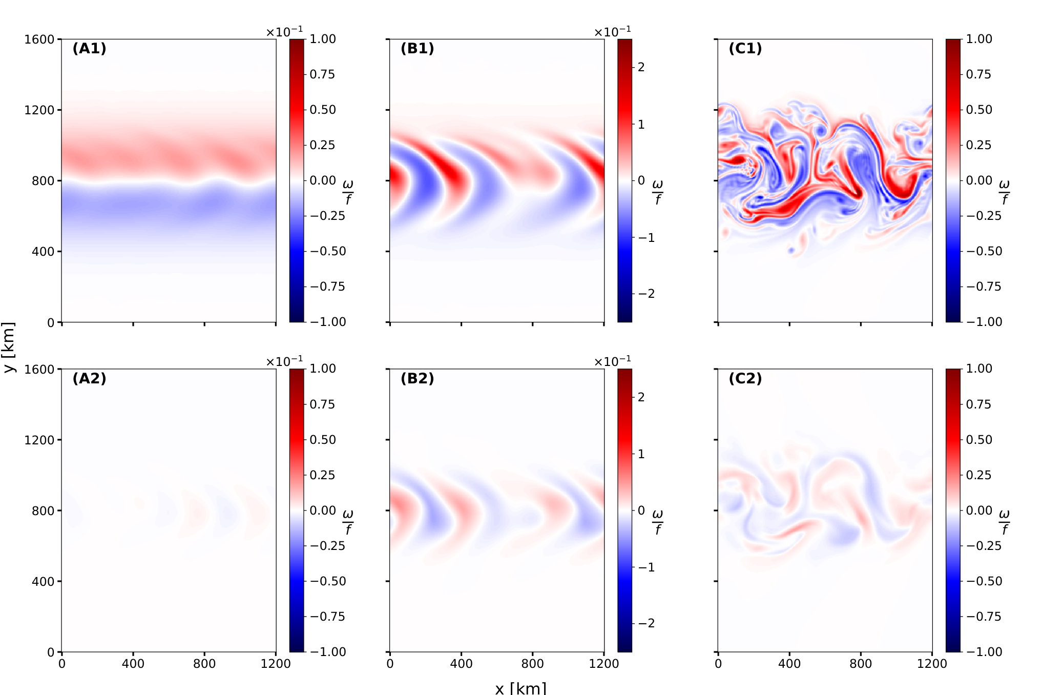
The simulation is run for 180 days, sufficiently long for the geostrophic turbulence to develop as a result of baroclinic instabilities. For our results, we analyze 100 snapshots taken every 2.5 hours starting from day 169. Spectra of ${\bf u}_{1}$ and $h_{1}$ are shown in Appendix Fig. 21. For our purpose, we only analyze the fields from the top layer since the flow in the bottom layer is much weaker. Hereafter, we drop the layer subcript since all results pertain to the top layer.

We compare $\overline{\tau}_{\ell}(h,{\bf u})$ with its approximation $\frac{1}{2}\ell^{2}\,M_{2}\,\partial_{k}\overline{h}\,\partial_{k}\overline{{\bf u}}$ in eq. (24c). We use a graded Top-Hat kernel following our previous work analyzing oceanic flow aluie2018mapping; Raietal2021,

where $\ell$ denotes the kernel width. This kernel is essentially the same as the Top-Hat in eq.(7), but with smoothed edges to avoid discretization noise from the nonuniform grids aluie2018mapping commonly used in general circulation models. Since the model domain is flat, $r$ is a simple Euclidean distance as in eq. (7), without complications due to Earth’s surface curvature aluie2019convolutions.

Fig. 8 compares the $\overline{\tau}_{\ell}({\bf u},h)$ at $\ell=100~$km with its approximation (24c). It indicates an excellent agreement. Fig. 9 (left column) shows a more quantitative evaluation of both components of the subscale transport approximation, where we can see that the approximation is remarkably accurate almost everywhere. Fig. 9 (right column) shows the joint PDFs between $\overline{\tau}_{\ell}({\bf u},\rho)$ and its approximation for both components (eastward and northward directions). They show correlations exceeding $0.95$. In Figs. 18-20 in the Appendix, we show similar comparisons at other length-scales of 50 km, 200 km, and 400 km. The joint PDF in Fig. 9 uses the z-scores of $\overline{\tau}_{\ell}$ and $\tau_{m}$, denoted by $\tau^{*}$ and $\tau^{*}_{m}$ and (all other figures show the actual $\overline{\tau}_{\ell}$ and $\tau_{m}$ values). As mentioned in eq. (33), the correlation coefficient between $\tau^{*}$ and $\tau^{*}_{m}$ is the same as that between $\overline{\tau}_{\ell}$ and $\tau_{m}$. We use z-scores to focus on how well the approximation $\tau_{m}$ is able to capture the exact subscale physics $\overline{\tau}_{\ell}$ up to a proportionality constant. For completeness, we plot the joint PDFs of the actual $\tau_{m}$ and $\overline{\tau}_{\ell}$ in Fig. 25 in the Appendix.

Noting that the spectral peak (Fig. 21) is at $\approx 300~$km, Fig. 10 plots the correlation coefficients between the exact $\overline{\tau}_{\ell}({\bf u},h)$ and its approximation (24c) as a function of $\ell$, which has values exceeding $0.90$ for scales $\ell$ smaller than the that of the spectral peak and decreasing to $\approx 0.75$ for scales $\ell=400~$km. These high correlation values justify our usage of expression (24c) as a proxy for $\overline{\tau}_{\ell}({\bf u},h)$ to gain insight into its underlying mechanics at least for scales $\ell$ smaller than that of the spectral peak.

The above result is a manifestation of the equivalence between transport by (i) flux due to an anti-symmetric diffusion tensor and (ii) an advective flux (Moffatt1983; MiddletonLoder1989; griffies1998gent). It suggests that coarse-grained simulations such as LES may need to solve

to represent the unresolved (subgrid) vorticity physics self-consistently.

${\bf J}(C)$ in eq. (45) can represent traditional subgrid models such as turbulent (Smagorinsky) diffusion smagorinsky1963general, ${\bf J}(C)=-\alpha_{turb}{\mbox{\boldmath$\nabla$}}\overline{C}_{\ell}$. The evaluation of ${\bf v}_{*}\sim{\mbox{\boldmath$\nabla$}}{\mbox{\boldmath$\times$}}({\mbox{\boldmath$\nabla$}}{\mbox{\boldmath$\times$}}\overline{{\bf u}}_{\ell})$ presents no additional cost since the resolved velocity $\overline{{\bf u}}_{\ell}$ is known. Figs. 17-26 in the Appendix show the joint PDFs of ${\bf v}_{*}$ and $\overline{{\bf u}}_{\ell}$ at different length-scales $\ell$, which demonstrate that ${\bf v}_{*}$ and the coarse velocity $\overline{{\bf u}}_{\ell}$ are often of a comparable magnitude.

Our interpretation of ${\bf v}_{*}$ as an eddy-induced velocity representing subscale vortical motions can be justified by appealing to a relation by Johnson⁴⁴ 4 Johnson’s relation (46) is exact only when filtering with a Gaussian kernel. johnson2020energy; johnson2021role,

Eq. (46) highlights that subscale flux $\overline{\tau}_{\ell}({\bf u},C)$ is due to the cumulative contribution of subscale velocity and scalar gradients at all scales $<\ell$. Since subscale velocity gradients can be decomposed into strain and vorticity, and since expression (24c) is the dominant contribution, we are justified in interpreting ${\bf v}_{*}$ as an eddy-induced velocity representing subscale vortical motions.

References

- [1] Gregory L Eyink. Multi-scale gradient expansion of the turbulent stress tensor. Journal of Fluid Mechanics, 549(-1):159, February 2006.
- [2] Pijush K Kundu, Ira M Cohen, and David R Dowling. Fluid mechanics. Academic press, 2015.
- [3] S. B. Pope. Turbulent flows. Cambridge University Press, New York, 2000.
- [4] C. Meneveau and J. Katz. Scale-Invariance and Turbulence Models for Large-Eddy Simulation. Ann. Rev. Fluid Mech., 32:1–32, 2000.
- [5] G. L. Eyink. Locality of turbulent cascades. Physica D, 207:91–116, 2005.
- [6] R S Strichartz. A guide to distribution theory and Fourier transforms. World Scientific Publishing Company, 2003.
- [7] Lawrence C Evans. Partial Differential Equations. Amer Mathematical Society, April 2010.
- [8] A. Leonard. Energy Cascade in Large-Eddy Simulations of Turbulent Fluid Flows. Adv. Geophys., 18:A237, 1974.
- [9] M Germano. Turbulence: the filtering approach. Journal of Fluid Mechanics, 238:325–336, 1992.
- [10] Ingrid Daubechies. Ten lectures on wavelets. SIAM, 1992.
- [11] Hussein Aluie. Coarse-grained incompressible magnetohydrodynamics: analyzing the turbulent cascades. New Journal of Physics, January 2017.
- [12] Gregory L Eyink. Review of the onsager” ideal turbulence” theory. arXiv preprint arXiv:1803.02223, 2018.
- [13] Fernando F Grinstein, Len G Margolin, and William J Rider. Implicit large eddy simulation, volume 10. Cambridge university press Cambridge, 2007.
- [14] Chad W Higgins, Marc B Parlange, and Charles Meneveau. The heat flux and the temperature gradient in the lower atmosphere. Geophysical research letters, 31(22), 2004.
- [15] H. Aluie. Scale decomposition in compressible turbulence. Physica D: Nonlinear Phenomena, 247(1):54–65, March 2013.
- [16] Dongxiao Zhao and Hussein Aluie. Inviscid criterion for decomposing scales . Physical Review Fluids, 3:054603, May 2018.
- [17] Massimo Germano. A proposal for a redefinition of the turbulent stresses in the filtered navier–stokes equations. The Physics of fluids, 29(7):2323–2324, 1986.
- [18] Andrey Nikolaevich Kolmogorov. The local structure of turbulence in incompressible viscous fluid for very large reynolds numbers. Dokl. Akad. Nauk SSSR, 30(4):299–303, 1941.
- [19] Alexander Mikhailovich Obukhov. The structure of the temperature field in a turbulent flow. Izv. Akad. Nauk. SSSR, Ser. Geogr. and Geophys., 13:58, 1949.
- [20] Stanley Corrsin. On the spectrum of isotropic temperature fluctuations in an isotropic turbulence. Journal of Applied Physics, 22(4):469–473, 1951.
- [21] Gregory L Eyink and Hussein Aluie. Localness of energy cascade in hydrodynamic turbulence. i. smooth coarse graining. Physics of Fluids, 21(11):115107, 2009.
- [22] Hussein Aluie and Gregory L Eyink. Localness of energy cascade in hydrodynamic turbulence. ii. sharp spectral filter. Physics of Fluids, 21(11):115108, 2009.
- [23] J Bardina, J H Ferziger, and W C Reynolds. Improved subgrid-scale models for large-eddy simulation. American Institute of Aeronautics and Astronautics, July 1980.
- [24] H. Aluie. Compressible Turbulence: The Cascade and its Locality. Phys. Rev. Lett., 106(17):174502, April 2011.
- [25] Michael Frazier, Michael W Frazier, Björn Jawerth, and Guido Weiss. Littlewood-Paley theory and the study of function spaces. Number 79 in Conference Board of the Mathematical Sciences regional conference series in mathematics. American Mathematical Society, Providence, Rhode Island, 1991.
- [26] H. Aluie and G. Eyink. Localness of energy cascade in hydrodynamic turbulence. II. Sharp spectral filter. Phys. Fluids, 21(11):115108, November 2009.
- [27] B. Vreman, B. Geurts, and H. Kuerten. Realizability conditions for the turbulent stress tensor in large-eddy simulation. J. Fluid Mech., 278:351–362, 1994.
- [28] P. Constantin, E. Weinan, and E. S. Titi. Onsager’s conjecture on the energy conservation for solutions of Euler’s equation. Communications in Mathematical Physics, 165:207–209, October 1994.
- [29] Robert A Clark, Joel H Ferziger, and William Craig Reynolds. Evaluation of subgrid-scale models using an accurately simulated turbulent flow. Journal of fluid mechanics, 91(1):1–16, 1979.
- [30] S Liu, C Meneveau, and J Katz. On the properties of similarity subgrid-scale models as deduced from measurements in a turbulent jet. Journal of Fluid Mechanics, 275:83–119, 1994.
- [31] Fernando Porté-Agel, Marc B Parlange, Charles Meneveau, and William E Eichinger. A priori field study of the subgrid-scale heat fluxes and dissipation in the atmospheric surface layer. Journal of the atmospheric sciences, 58(18):2673–2698, 2001.
- [32] Branko Kosović. Subgrid-scale modelling for the large-eddy simulation of high-reynolds-number boundary layers. Journal of Fluid Mechanics, 336:151–182, 1997.
- [33] Freddy Bouchet. Parameterization of two-dimensional turbulence using an anisotropic maximum entropy production principle. arXiv preprint cond-mat/0305205, 2003.
- [34] A Leonard. Large-eddy simulation of chaotic convection and beyond. In 35th Aerospace Sciences Meeting and Exhibit, page 204, 1997.
- [35] V Borue and S A Orszag. Local energy flux and subgrid-scale statistics in three-dimensional turbulence. Journal of Fluid Mechanics, 366(1), 1998.
- [36] Perry L Johnson. Energy transfer from large to small scales in turbulence by multiscale nonlinear strain and vorticity interactions. Physical review letters, 124(10):104501, 2020.
- [37] Perry L Johnson. On the role of vorticity stretching and strain self-amplification in the turbulence energy cascade. Journal of Fluid Mechanics, 922, 2021.
- [38] Hyung Suk Kang and Charles Meneveau. Passive scalar anisotropy in a heated turbulent wake: new observations and implications for large-eddy simulations. Journal of Fluid Mechanics, 442:161–170, 2001.
- [39] Sergei G Chumakov. A priori study of subgrid-scale flux of a passive scalar in isotropic homogeneous turbulence. Physical Review E, 78(3):036313, 2008.
- [40] Aarne Lees and Hussein Aluie. Baropycnal work: a mechanism for energy transfer across scales. Fluids, 4(2):92, 2019.
- [41] Shriram Jagannathan and Diego A Donzis. Reynolds and Mach number scaling in solenoidally-forced compressible turbulence using high-resolution direct numerical simulations. Journal of Fluid Mechanics, 789:669–707, February 2016.
- [42] Christoph Federrath, Ralf S. Klessen, and Wolfram Schmidt. The density probability distribution in compressible isothermal turbulence: Solenoidal versus compressive forcing. The Astrophysical Journal Letters, 688(2):L79, 2008.
- [43] V Eswaran and SB Pope. An examination of forcing in direct numerical simulations of turbulence. Computers & Fluids, 16(3):257–278, 1988.
- [44] Alistair Adcroft, Whit Anderson, V Balaji, Chris Blanton, Mitchell Bushuk, Carolina O Dufour, John P Dunne, Stephen M Griffies, Robert Hallberg, Matthew J Harrison, et al. The gfdl global ocean and sea ice model om4. 0: Model description and simulation features. Journal of Advances in Modeling Earth Systems, 11(10):3167–3211, 2019.
- [45] Stephen M Griffies, Alistair Adcroft, and Robert W Hallberg. A primer on the vertical lagrangian-remap method in ocean models based on finite volume generalized vertical coordinates. Journal of Advances in Modeling Earth Systems, 12(10):e2019MS001954, 2020.
- [46] Robert Hallberg. Using a resolution function to regulate parameterizations of oceanic mesoscale eddy effects. Ocean Modelling, 72:92–103, 2013.
- [47] Norman A Phillips. Energy transformations and meridional circulations associated with simple baroclinic waves in a two-level, quasi-geostrophic model. Tellus, 6(3):274–286, 1954.
- [48] GK Vallis. Atmospheric and oceanic fluid dynamics: fundamentals and large-scale circulation, 2006.
- [49] Stephen M Griffies and Robert W Hallberg. Biharmonic friction with a smagorinsky-like viscosity for use in large-scale eddy-permitting ocean models. Monthly Weather Review, 128(8):2935–2946, 2000.
- [50] Peter R Gent and James C Mcwilliams. Isopycnal mixing in ocean circulation models. Journal of Physical Oceanography, 20(1):150–155, 1990.
- [51] Hussein Aluie, Matthew Hecht, and Geoffrey K Vallis. Mapping the energy cascade in the north atlantic ocean: The coarse-graining approach. Journal of Physical Oceanography, 48(2):225–244, 2018.
- [52] Shikhar Rai, Matthew Hecht, Matthew Maltrud, and Hussein Aluie. Scale of oceanic eddy killing by wind from global satellite observations. Science Advances, 7(28):eabf4920, 2021.
- [53] Hussein Aluie. Convolutions on the sphere: commutation with differential operators. GEM-International Journal on Geomathematics, 10(1):9, 2019.
- [54] H.K. Moffatt. Transport effects associated with turbulence with particular attention to the influence of helicity. Reports on Progress in Physics, 46:621–664, 1983.
- [55] J. F. Middleton and J. W. Loder. Skew fluxes in polarized wave fields. Journal of Physical Oceanography, 19:68–76, 1989.
- [56] Stephen M Griffies. The gent–mcwilliams skew flux. Journal of Physical Oceanography, 28(5):831–841, 1998.
- [57] Joseph Smagorinsky. General circulation experiments with the primitive equations: I. the basic experiment. Monthly weather review, 91(3):99–164, 1963.
- [58] Daniel Livescu. Turbulence with large thermal and compositional density variations. Annual Review of Fluid Mechanics, 52:309–341, 2020.
- [59] Mahmoud Sadek and Hussein Aluie. Extracting the spectrum of a flow by spatial filtering. Physical Review Fluids, 3(12):124610, December 2018.
- [60] Michele Buzzicotti, Benjamin A Storer, Stephen M Griffies, and Hussein Aluie. A coarse-grained decomposition of surface geostrophic kinetic energy in the global ocean. Earth and Space Science Open Archive, page 58, 2021.
Appendix
V.1 Additional supporting material from the compressible turbulence simulation
V.2 Additional supporting material from the shallow water simulation