A Bayesian Approach for Spatio-Temporal Data-Driven Dynamic Equation Discovery
Joshua S. North11 1 Corresponding author: jsnorth@lbl.gov, Earth and Environmental Sciences, Lawrence Berkeley National Laboratory, Berkeley, CA, 1 Cyclotron Road, Christopher K. Wikle22 2 wiklec@missouri.edu, Department of Statistics, University of Missouri, Columbia, MO, 146 Middlebush Hall, Erin M. Schliep33 3 emschlie@ncsu.edu, Department of Statistics, North Carolina State University, Raleigh, NC, 2311 Stinson Drive
Abstract
Differential equations based on physical principals are used to represent complex dynamic systems in all fields of science and engineering. Through repeated use in both academics and industry, these equations have been shown to represent real-world dynamics well. Since the true dynamics of these complex systems are generally unknown, learning the governing equations can improve our understanding of the mechanisms driving the systems. Here, we develop a Bayesian approach to data-driven discovery of non-linear spatio-temporal dynamic equations. Our approach can accommodate measurement noise and missing data, both of which are common in real-world data, and accounts for parameter uncertainty. The proposed framework is illustrated using three simulated systems with varying amounts of observational uncertainty and missing data and applied to a real-world system to infer the temporal evolution of the vorticity of the streamfunction.
Key Words: Bayesian Dynamic Discovery, Data-Driven Discovery, Nonlinear Dynamic Equation, Partial Differential Equation
1 Introduction
Dynamic equations (DE) parameterized by partial differential equations (PDE) – an equation relating a partial derivative of a variable to a function of its current state – are used across all fields of science and engineering to describe complex processes. DEs encode physical processes by a set of mathematical equations, enabling complex systems such as the spread of infectious disease (Bolker and Grenfell, 1995; Mangal et al., 2008; Kühnert et al., 2014), evolution of invasive species (Hastings, 1996; Liu et al., 2019), weather and climate (Charney et al., 1950; Holton and Hakim, 2012), and the flow of fluids (White and Majdalani, 2006) to be characterized and modeled (see also Higham et al., 2016, for further discussion). Given that any real world process is only approximately characterized by mathematical relationships, mathematically derived DEs are inherently unable to completely characterize a real world system. This suggests the need to use observations of the real world system to better characterize the underlying DEs.
Recently, there has been a push to use data to discover the governing equations in these complex systems. Originally proposed using symbolic regression (Bongard and Lipson, 2007; Schmidt and Lipson, 2009), the focus has since shifted to either sparse regression or deep modeling. The original sparse regression approach, termed Sparse Identification of Nonlinear Dynamics (Brunton et al., 2016, SINDy;), used numerical differentiation to construct a response that is regressed against a library of functions that potentially govern the system. Through sparse regression, either with an penalization term (Tibshirani, 1996) or using a thresholding approach (Zheng et al., 2019; Champion et al., 2020), key terms governing a variety of ordinary differential equations (ODE) are identified. Using the fundamental idea of SINDy, the framework was extended to include PDEs and parametric forms (Schaeffer, 2017; Rudy et al., 2017; Rudy et al., 2019a; Rudy et al., 2019b), stochastic dynamical systems (Boninsegna et al., 2018), uncertainty quantification of the parameters (Zhang and Lin, 2018; Yang et al., 2019; Niven et al., 2020; Fasel et al., 2021; Hirsh et al., 2021), and has been incorporated into a Python package (de Silva et al., 2020, PySINDy;).
Deep models used for data-driven discovery of dynamics can broadly be grouped into two categories – approximating dynamics (Raissi et al., 2017; Raissi and Karniadakis, 2018; Raissi et al., 2020; Sun et al., 2019; Wu and Xiu, 2020) and discovering dynamics (Both et al., 2021; Xu et al., 2019; Xu et al., 2020; Xu et al., 2021; Long et al., 2017; Long et al., 2019). Using deep models to approximate the dynamics of complex systems enables a computationally inexpensive method to obtain measurements of otherwise difficult to simulate systems while still obeying physical principles (see Reichstein et al., 2019, for an in-depth discussion on the topic). However, our goal is the discovery of the governing equations where “data-driven discovery” refers to the discovery of the functional form of the system and deep models have also been used in this context. Combining deep modeling and sparse identification, Both et al., 2021 approximate the PDE using a neural network, which is used to compute derivatives and construct a sparse formulation similar to the SINDy approach. Long et al., 2017; Long et al., 2019 use a symbolic neural network, an extension of symbolic regression, and a numerical approximation of differential operators in a feed-forward network to discover PDEs and Xu et al., 2021 use a fully connected neural network with a genetic algorithm to express and generate terms of a PDE.
Two open problems in data-driven discovery are (i) accounting for measurement uncertainty (i.e., missing data and measurement noise) and (ii) parameter uncertainty. Existing methods that extend the SINDy framework to account for uncertainty quantification employ either a bootstrap approach (Fasel et al., 2021) or a Bayesian approach with variable shrinkage/selection priors placed on the coefficients associated with the library terms (Zhang and Lin, 2018; Niven et al., 2020; Hirsh et al., 2021). These approaches directly follow the first steps of the SINDy framework, where derivatives are computed numerically, data is de-noised, and the feature library is constructed. In this manner, the true uncertainty associated with the observed data is ignored; the estimate for the system uncertainty is now dependent on the numerical differentiation method, which subsequently influences the estimate of the parameter uncertainty. Yang et al., 2020 developed a method to jointly account for uncertainty in the observed data and parameters based on differential Bayesian programming. While this approach directly accounts for measurement uncertainty, it requires derivatives be computed using a numerical solver (e.g., Runge-Kutta), which can lead to numerical instabilities and cannot accommodate missing data.
To account for observational uncertainty and missing data when modeling complex non-linear systems, statisticians have incorporated dynamic equations parameterized by PDEs into Bayesian hierarchical models (Berliner, 1996; Royle et al., 1999; Wikle et al., 2001, BHM;). These models, sometimes called physical statistical models (PSM), enable modeling mechanistic relationships within a probabilistic framework (see Berliner, 2003; Cressie and Wikle, 2011; Kuhnert, 2017, for an overview). PSMs are composed of three sub-models – data, process, and parameter models. To account for observational and mechanistic uncertainty, PSMs consider the dynamics to be latent in the process stage, and represent the observed data in the data stage conditioned on these latent dynamics. While PSMs have been used to model and better understand complex systems, such as ocean surface winds (Wikle et al., 2001; Milliff et al., 2011) and the spread of avian species (Wikle, 2003; Hooten and Wikle, 2008), they require the dynamic relationships (although not weights/parameters associated with those relationships) to be specified a priori. To increase flexibility for representing complex processes, PSMs consider the parameters that describe the influence of dynamic components to be random, and often allow them to have spatial or temporal dependence, enabling the model to adapt to the data. While PSMs are adaptable to a variety of problems and provide inference on how the process may be evolving, they cannot be used to discover new dynamical relationships.
Recently, North et al., 2022 proposed a Bayesian data-driven discovery method that accounts for observational and parameter uncertainty using a BHM framework composed of data, process, and parameter models for ODEs. Analogous to PSMs, the dynamics are modeled as a latent process and observational error is accounted for in the data model. Allowing the dynamics to be a latent random process is different than previous data-driven discovery methods that attempt to quantify uncertainty. To link the dynamic system to its derivatives probabilistically, the dynamic process and all the derivatives are modeled using a basis expansion with a common set of basis functions. Derivatives are then obtained analytically using the basis expansion, which incorporates dependence between the dynamic process and its derivatives. A library of potential functions can be constructed based on the basis coefficients and functions, and a variable selection prior is used to identify the key functions governing the non-linear system.
Here, we propose a spatio-temporal extension to Bayesian data-driven discovery for PDEs. The general framework follows North et al., 2022, however the addition of the spatial dimension requires a reformulation of the process model. To account for the extra dimension (i.e., space), we model the dynamic process as a higher-order tensor where the dimensions represent space, time, and the number of components (sometimes called the system states) in the system. The tensor is decomposed using differentiable basis functions in space and time, probabilistically linking the dynamic system with its spatial and temporal derivatives. The basis decomposition is incorporated into the BHM, enabling potential functions to be constructed using the basis functions and coefficients. A variable selection prior on the coefficients produces a sparse solution set and the resulting system. In contrast to the ODE discovery problem, the library of potential functions for PDEs can exhibit strong multicollinearity. An additional contribution of this work is an approach to account for multicollinearity in high dimensional, dynamic systems.
We demonstrate our method using data generated from Burgers’ equation, the heat equation, and a predator-prey reaction-diffusion equation with varying levels of measurement noise. In addition, we demonstrate our model’s ability to accommodate missing data using Burgers’ equation. The simulations show that our approach is robust to measurement noise and missing data, able to learn the dynamics of complex systems, and provides formal uncertainty quantification on parameter estimates and the confidence of the discovered dynamics. Last, we apply our method to infer the evolution of atmospheric vorticity over time having only observed the streamfunction and obtain results that coincide with geophysical balances (i.e., the barotropic vorticity equation).
The remainder of this paper is organized as follows. In Section 2 we define the tensor and derivative notation used throughout the manuscript. In Section 3 we give background on the general dynamic system, showcase how inference on the derivative of the system is made, and present the Bayesian hierarchical model. In Section 4 we describe parameter estimation and discuss modeling choices. In Section 5 we demonstrate our method on multiple simulated data sets and in Section 6 we perform inference on a real-world system. Section 7 concludes the paper.
2 Preliminary Notation
In this section we define tensor and derivative notation. All variables in this section are used only for illustrating notation. Problem specific notation will be introduced in Section 3.
2.1 Tensor Notation
PDEs are commonly defined over multiple dimensions (e.g., space, time, components), and benefit from the use of higher-order tensor notation when the number of dimensions is three or more. We generally follow the notation of Kolda and Bader, 2009 and refer the reader to their work for more details and references of tensor notation and applications.
Let be a tensor of order where the element is denoted by . A slice of the tensor is a two-dimensional section where all but two indices are held constant. For example, the horizontal, lateral, and frontal slices of the third order tensor are denoted by , , and , respectively. A tensor can be converted to a matrix using -mode matricization (also known as unfolding or flattening). The -mode matricization of the tensor , denoted by , arranges the mode fibers (the higher-order equivalent of matrix rows and columns) to be columns in the resulting matrix. For example, the possible modes of are , , and . In general, we will only be concerned with the mode-3 matricization of a tensor and will denote in place of (all other modes will be properly denoted).
To multiply a tensor by a matrix , we use the -mode product (i.e., multiply a tensor by a matrix or vector in mode ). The -mode product of the tensor and matrix is denoted as and is of size . Equivalently, in terms of unfolded (matricized) tensors, .
2.2 Tensor Basis Representation
Let be the order 3 tensor from Section 2.1. Define the expansion of the element of as
where , , and are basis functions and is the tensor of associated basis coefficients. To reduce the dimension, we keep the first , and terms from , and , and define each basis function at discrete values , , and , respectively. That is, let
where is the vector outer product, is a , is a , and is a matrix of basis coefficients where each column is given by , , and , and is shorthand notation introduced in Kolda, 2006. Our basis decomposition is similar to the Tucker decomposition (Tucker, 1966), except we assume and are known and our goal is to estimate . Note, we provide the expansion only for an order 3 tensor (sufficient for this manuscript), but the concept can be extended to higher order tensors.
2.3 Derivative Notation
As discussed in Section 1, we propose a method to discover the governing equations in PDEs. As the name suggests, a PDE is composed of partial derivatives of some variable that is indexed in space or time or both. We denote partial derivatives using a subscript, for example , , , and so forth. We denote the th order of a derivative generally as . In order to disambiguate notation, we denote the index of a vector/matrix/tensor using parentheses (e.g., ), reserving the subscript to denote derivatives.
Within the PDE literature there are different choices of notation to denote the same operation. For example, the Laplacian operator can be denoted as . Wherever an operator such as the Laplacian is used for the first time, we will define it. This may result in our notation differing from other texts, but we aim to be consistent within the paper.
3 Bayesian Dynamic Equation Discovery
Here we propose a general hierarchical model for making inference on nonlinear spatio-temporal dynamic systems. We begin by motivating the general class of PDEs and manipulate them to fit within a statistical framework.
3.1 Dynamic Equations
Consider the general PDE dynamic system describing the evolution of a continuous field
| (3.1) |
where the vector denotes the realization of the -dimensional system at location and time (e.g., ), represents the (potentially nonlinear) evolution function, and represents any covariates that might be included in the system. Here, is a spatial location in the domain with , and is the temporal realization of the system where . We define (3.1) in two dimensions (i.e., and ), but the problem can be simplified to one dimension (i.e., and ) or generalized to higher spatial dimensions. Finally, as is common in the dynamic systems literature, we refer to the -dimensional multivariate vector as the state or system state, and use the term component to refer to each of the elements of .
We reparameterize 3.1 to be intrinsically linear (in parameters) as
| (3.2) |
where is a sparse matrix of coefficients and is a vector-valued nonlinear transformation function of length . The input of the arguments for are general and contain anything that potentially relates to the system. For example, this could include terms describing advection, diffusion, dispersion and growth, polynomial functions and interactions, or sinusoidal functions, and are chosen based on a general mechanistic understanding of the system. This results in being quite large and (3.2) has the potential to be highly over-parameterized. Thus, we will employ regularization to induce sparsity in the matrix .
As an example of a classic PDE within our framework, consider the reaction diffusion equation
where represents the densities of two processes, is a diagonal matrix where are the diffusion constants, and are (non)linear reaction functions. The reaction-diffusion equation can be used to model the densities of prey () and predator () populations (Hastings, 1996). For a predator-prey model, a possible choice for the reaction function is , a simplistic representation of the Lotka-Volterra system where and represent the prey’s birth and predation rates, respectively, and and represent the predator death and kill success rates. Following (3.2), and suppressing the spatial and temporal indices, we have
Typically we do not know and instead highly over-parameterize by including a library of potential terms and select against the coefficients in to identify relevant terms.
In real-world problems, (3.2) does not hold exactly. Stochastic forcing could perturb the system (e.g., weather systems, demographic stochasticity) or there could be error in the model specification. We accommodate this unknown stochasticity by including an additive error term
| (3.3) |
where, for example, is a mean zero Gaussian process with variance/covariance matrix . In general, spatial or temporal dependencies could be considered in this error term.
To represent (3.3) using tensor notation, let where is the tensor of the dynamic process. Similarly, let be the function evaluated at each location in space-time and is the space-time-component uncertainty tensor. The tensor formulation of (3.3) in then
| (3.4) |
This forms the core of our process model, where we relate the temporal derivative of some space-time-component process to a nonlinear function of its current state. While not explicitly stated in (3.4), is still a function of the state process .
3.2 Basis Representation
As described in Section 2.2, we can represent the tensor using basis functions. Decomposing in terms of a finite collection of spatial, temporal, and component basis functions, we write
where , , , and . Here, , and are matrices of spatial, temporal, and component basis functions, respectively, and is a tensor of basis coefficients (traditionally called the core tensor).
We can obtain derivatives of the elements of analytically by taking derivatives of the basis functions. Specifically, let and be matrices of basis functions differentiable up to at least the highest order considered in (3.1). We then compute spatial and temporal derivatives of by computing the derivatives of and . That is, denote , , , and so forth. Derivatives of are then computed as
| (3.5) | ||||
and so forth. Representing (3.4) using the basis decomposition, we have
where may include truncation error. While not explicitly stated, now depends on , and .
Proposition 1
The mode-3 decomposition of where in space and time at location and time is
where is a matrix of basis coefficients, is a length- vector of spatial basis functions, is a length- vector of temporal basis functions, and is a matrix of component basis functions.
Proof. See supplementary material.
Decomposing (3.4) in terms of basis functions and taking the mode-3 matricization accomplishes two tasks. First, this enables inference on derivatives of the process when only the process is known (e.g., see (3.5)). Second, keeping fewer basis functions than observations (e.g., , ) allows the reconstruction of to be smooth (Wang et al., 2016).
Note, we include for generality in the construction of our method. While one could specify in terms of basis functions, our goal is not to reduce the dimension of the system state variables. In our analyses, we choose to be the identity matrix.
3.3 Transformation of Derivative
Up to this point, we have considered PDEs that relate the temporal derivative (of some order ) of the continuous surface on left-hand side (LHS) of (3.1) to a function of its current state on the right-hand side (RHS) of (3.1). However, equations with a spatio-temporal derivative of on the LHS are common (Higham et al., 2016, e.g., vorticity equation,). For example, the LHS of (3.1) could depend on the Laplacian operator, where .
To be more general, we now allow the LHS of (3.1) to be a function of spatio-temporal derivatives of and consider the more general PDE
| (3.6) |
where is some linear differential operator. The original PDE (3.1) is a special case of (3.6) where is the identity function.
Proposition 2
Let be a linear differential operator. The basis formulation of a PDE with a space-time function on the LHS is
Proof. See supplementary material.
3.4 Data Model
We assume is an observation of the -dimensional latent process outlined in Section 3.2 with some unknown measurement uncertainty. We model using a generalization to the traditional linear data error model that links the dynamics to the observed process (e.g., see Cressie and Wikle, 2011, Chapter 7). That is, we model
| (3.8) |
where , is the incidence matrix that maps from to , and uncertainty in the observations of the process are captured by . The dimension of the data, , is allowed to vary based on the space-time location due to potentially missing data and we assume the errors are independent in space and time.
Within the hierarchical model, missing data are accommodated by allowing the dimension of the incidence matrix, , to vary in time. Since missing data are handled in the data model and the latent process is fully specified, missing data do not impact the process model specification. If there are no missing data at time and location , then and . When one or more system components are missing data, the row corresponding to the missing system component is removed. For example, if we have a three-dimensional system, say and the observation component for is missing at location and time , then
See Chapter 7 of Cressie and Wikle, 2011 for more discussion of this approach for accommodating missing observations in hierarchical spatio-temporal models.
Incorporating the basis expansion of the process in (3.8), at location and time ,
| (3.9) |
where and now accounts for the discrepancy between the “true” underlying process and our approximation using the basis formulation.
3.5 Parameter Model
The data and process equations correspond to the first and second level of our hierarchical model, respectively. For convenience, we restate (3.9) and (3.7) for location and time
where and . For clarity, we present the details on the model parameters in Table 1. Our goal is to make inference on the unknown parameters , and . The sparse matrix identifies the nonlinear dynamic equation, captures the error dependencies within the dynamic equation, captures the measurement uncertainty associated with the observed process, and defines the smooth latent process.
| Model | Symbol | Description | Dimension |
| Variable | |||
| Data | Observed data | ||
| Data | Mapping matrix | ||
| Data | Data uncertainty distribution | ||
| Data | Measurement error covariance matrix | ||
| Process | Dynamic process | ||
| Process | Basis coefficient tensor | ||
| Process | Basis coefficient matrix (mode-3) | ||
| Process | spatial basis function for location | ||
| Process | th order temporal basis function for time | ||
| Process | component basis function matrix | ||
| Process | Dynamic evolution matrix | ||
| Process | Feature library | ||
| Process | Process uncertainty distribution | ||
| Process | Dynamic equation error covariance matrix | ||
| Dimension | |||
| Number of observed time points | 1 | ||
| Number of observed spatial locations | 1 | ||
| Dimension of observation vector at time and location | 1 | ||
| Dimension of latent process (dynamic system) | 1 | ||
| Number of library functions | 1 | ||
| Number of spatial basis functions | 1 | ||
| Number of temporal basis functions | 1 | ||
| Number of component basis functions | 1 | ||
| Highest order derivative in the dynamic system | 1 | ||
| Indices | |||
| Time interval, , | 1 | ||
| Spatial location, , | 1 | ||
| Order of the derivative, | 1 |
To complete our Bayesian hierarchical model, we define the following priors on these parameters. We use the spike-and-slab prior (Mitchell and Beauchamp, 1988; George et al., 1993) to induce sparsity into . We write
where denotes coefficient of component , is a matrix of inclusion indicators of the same dimension as , denotes the Dirac function at 0, is the th diagonal component of , , and . That is, if a variable is not included (i.e., ), then the corresponding element is zero. If a variable is included (i.e., ), then the corresponding element is non-zero. There are multiple choices for the prior . We specify the g-slab prior corresponding to Zellner’s g-prior (Zellner, 1986) where is taken to be the size of the data. See Malsiner-Walli and Wagner, 2016 for other potential choices and further discussion.
While other shrinkage/selection priors could be used, such as Stochastic Search Variable Selection (George et al., 1993, SSVS;), LASSO (Park and Casella, 2008), or Horseshoe (Carvalho et al., 2010), we found the spike-and-slab to be preferable since it performs well with correlated predictors (Ročková and George, 2014), which is generally present in the feature library (see Section 4). Additionally, the posterior summary of the latent variable gives the inclusion probability for each component of , providing further insight into the certainty of the recovered system. For all examples presented below, we determine the identified system as composed of terms that are included with at least 50% posterior probability. However, this threshold is subjective and one could choose a different value depending on their specific application.
To estimate and avoid reducibility of the Markov chain, we compute the marginal posterior distribution , which is obtained by integrating over the parameters subject to selection. That is,
To make the integration analytically tractable and keep conjugacy in the model, we restrict to be diagonally structured where and each diagonal element is assigned the non-informative prior . Then, the probability any element is included is given as
| (3.10) |
where
In situations where dependence between the components is required, a different prior could be used.
There is potential for elements of the variance-covariance matrix to have small values. Inference using traditional conjugate Inverse Gamma/Wishart priors are overly sensitive to the choice of hyperpriors when estimates are small (Gelman, 2006). Instead, we use the conjugate Half-t prior proposed by Huang and Wand, 2013 for covariance estimation, which imposes less prior information and does not have as strong of influence on small estimates. We restrict the measurement error to be diagonally structured since it is often a reasonable assumption that measurement noise is independent (Cressie and Wikle, 2011) (although this restriction can be removed if warranted). Let , where each diagonal element, , is assigned a conjugate Half-t prior.
Finally, in order to induce sparcity in the basis coefficients, we assign a Bayesian elastic net prior (Li and Lin, 2010) to . Specifically, our prior is
where are penalty parameters. The elastic net prior helps regularize the basis coefficients against basis functions. While it is possible to specify hyperpriors for the two penalty terms, we find inference is not overly sensitive to the choice of penalty parameters and fix them each to a small value (e.g., 0.01 or 0.001).
4 Model Estimation
Our goal is to obtain samples from the joint posterior distribution . We achieve this by sampling from the five full-conditional distributions , , , , and (see the supplementary material for the details of the distributions and sampling algorithm) using a Markov chain Monte Carlo (MCMC) sampling scheme. The four components and are updated using classical Bayesian methods and is updated using a stochastic gradient approach. Due to the variety of problems for which our method is applicable, some modeling choices are case specific. Additionally, some aspects of the implementation of the MCMC framework warrant a more detailed discussion. The following sections provide additional information pertaining to these model specifications and procedures.
4.1 Basis Coefficient Estimation
The basis coefficients, , completely define the latent process and all derivatives in both space and time, meaning proper estimation is crucial to the discovery process. Since is embedded within the nonlinear function (see Proposition 1) and is problem specific, it is difficult to estimate. To accommodate a generically specified , we use an adapted version of stochastic gradient descent (SGD) with a constant learning rate (Mandt et al., 2016, SGDCL;). Whereas other approaches to estimate (e.g., Expectation-Maximization or Metropolis-Hastings) could be used, SGDCL provides important advantages – a conjugate updating scheme and a reduced computational cost for any specification of .
As with SGD, SGDCL relies on the gradient of a loss function and a learning rate. For SGDCL, the loss function is the negative log posterior for our parameters of interest, . The loss function at location and time is
To simplify notation, denote and . Then, the gradient of the loss function , for location and time is
where generically denotes .
SGDCL (Mandt et al., 2016) replaces the true gradient with the stochastic estimate,
where is a random subset of the observations, called a mini-batch, and is the cardinality of the set. Within the context of a MCMC algorithm, the th update of is given by
where denotes a random minibatch specific to the update and is the learning rate. To accommodate different scales for each component, we allow to be a vector of length where each component can have a specific learning rate.
The final challenge to estimating is computing . Because is problem specific, is also problem specific. One option is to use automatic differentiation (AD) to analytically compute the derivative of . There are many different libraries and programs that perform AD, and we explored the use of the ForwardDiff (Revels et al., 2016) package in Julia (Bezanson et al., 2017) with success. However, there is computational overhead to AD. For all the examples presented here we computed without AD for each problem to mitigate this computation bottleneck.
4.2 Choice of Basis Functions
The choice of basis functions are subjective and have the potential to affect the model fit (North et al. 2022). Furthermore, the choices of spatial and temporal basis functions do not need to be the same (e.g., radial basis functions in space and Fourier basis functions in time). There are other choices regarding basis functions that need to be taken into consideration (see Ramsay and Silverman, 2005, Chapter 3 for a discussion on how to choose basis functions based on the “shape” of the data). The most important requirement is that the spatial and temporal basis functions need to be differentiable up to at least the highest order spatial and temporal derivative considered, respectively. We found local basis functions (e.g., B-splines) perform better than global basis functions (e.g., Fourier basis functions) (North et al., 2022, see), especially when there are local regions with minimal curvature. For these reasons, we use B-splines of an order greater than our highest derivative (in both space and time). In choosing how many basis functions to use, enough need to be included such that the estimated solution curve is flexible, the dynamics are captured, and the posterior latent space is properly explored, but not so many such that unnecessary noise is introduced into the system. Empirically, we found a ratio of approximately 1 basis function to every 3 to 5 observations to work well.
4.3 Choice of Feature Library
The choice of functions for the feature library is crucial to the identification of the system. Our method is restricted to search over a predefined set of functions, meaning that our method is unable to identify an important function if it is not included in the library. For this reason, it is best to over-parameterize the feature library (and hence ) instead of specifying a restrictive set of functions. Additionally, some knowledge of the problem is beneficial (i.e., this is not a black-box approach). Having an understanding of the potential dynamics a priori can assist in the recovery of important dynamics. For example, if the system appears to diffuse over time, then a diffusion term should be included. A good default choice is polynomial terms that interact with varying orders of spatial and/or temporal derivatives of the process (e.g., see the library for Burgers’ example) as this will cover a wide collection of systems.
With regard to the choice of in (3.6) and (3.7), scientific knowledge of the problem is required. The choice of is not searched over as with the library terms; rather it is pre-specified. For example, in our real-world example, the a prior goal was to make inference on the change of atmospheric vorticity with time, and vorticity can be represented as the Laplacian of the streamfunction. Because this transformation function is not learned, it is a modeling choice that is user specified (the default is the identity as in Proposition 1).
4.4 Multicollinearity in Library
A major issue facing the identification of spatio-temporal dynamic equations is multicollinearity in the feature library. Figure 1 shows the correlation between different components of a library using data generated from Burgers’ equation. In this example, the polynomial terms, and , are very positively linearly correlated , posing a challenge to parameter inference. As with classical regression, multicollinearity has the potential to introduce bias into the coefficient estimates, including altering their sign. While the spike-and-slab has been shown to perform well with correlated variables, as discussed in Section 3.5, the problem still persists and can pose an estimation issue in problems similar to the example using Burgers’ equation.

This issue originates from the over-inflation of minor reductions in the residual sum of squares (RSS) when a highly correlated, but incorrect term, is included. Specifically, the probability of including any term in the library (3.10) is dependent on the ratio of the residual sum of squares for the model with the term included () to the model without the term included () through the value of . That is, under the -prior
Because , the ratio is bound between 0 and 1, where correct terms in the library result in the ratio being closer to 0 and incorrect terms result in the ratio being close to 1. However, as the ratio is raised to a power of (proportional to the number of observations), the value of goes to 0 as the number of observations goes to infinity, resulting in all variables being found significant. This issue is exacerbated by correlated variables, especially if there are multiple confounding variables where the system can be approximated by some linear combination of the feature library without the true terms being included.
To combat this issue we propose a method to reduce the impact of correlated variables (i.e., variables where in the ratio of RSSs being close to 1 are found significant). For this, we subsample the process when estimating the inclusion latent variable . That is, to compute (3.10) within each iteration of the Gibbs sampler, we randomly sample the process. This results in
where and are the size of the subsampled dimensions. We provide details on how to choose the subsample size and our choices for the examples in the supplementary material. Note that this subsampling is only done for the update step of the algorithm.
5 Simulations
We show our proposed model is able to discover dynamic equations using data simulated from three well known systems – Burgers’ equation, the heat equation, and a reaction-diffusion system. For all three examples, we investigate the impact of measurement noise on inference. We simulate measurement noise by adding mean zero Gaussian errors to the state vector. Specifically, we let , where is the simulated data, is the additive noise, is the standard deviation of the simulated process , and is the percent of noise ranging from 0 to 1. In addition, we show how the model performs when data are missing sporadically for Burger’s equation. Unless otherwise stated, all reported estimates are rounded to three significant digits for readability. For all simulations and real-world examples, we obtain 5000 posterior samples and discard the first 2500 as burn-in. Convergence is assessed visually via trace plots with no issues detected.
5.1 Burgers’ Equation
Burgers’ equation is a simplification of the Navier-Stokes equations, describing the speed of a fluid at a location in space and time (Bateman, 1915; Burgers, 1948). We consider Burgers’ equation in one spatial dimension defined by the nonlinear PDE
where is the speed of the fluid at location and time and is the viscosity of the fluid. Data are generated using spectral differentiation and the Tsit5 (Tsitouras, 2011) numerical solver from the Julia package DifferentialEquations.jl (Rackauckas and Nie, 2017) with initial condition . The simulated data consist of 256 spatial locations across 101 time points where and (Figure 2). We consider four cases – no measurement noise, 2% measurement noise, 5% measurement noise, and 2% measurement noise with 5% of data missing at random.

For all four cases we specify the model with and define the feature library as
After obtaining posterior samples, we keep only terms with greater than a 50% inclusion probability to be included in the identified equation. The recovered equations and 95% highest posterior density (HPD) interval without and with measurement noise for the included terms are shown in Table 2. In all four scenarios, the true components of the dynamic system are correctly identified. In addition, the probability of including extraneous terms from the feature library is low in each scenario (see Supplementary material Table 1), giving confidence to our identified equation.
The credible intervals of all parameters cover the true value with the exception of in the cases with 5% noise and 2% noise with 5% missing data. In addition, no extraneous terms are identified in any scenario. The probability of including another term ( for all four cases) is low, giving us relative certainty that the identified equation is indeed correct. Clearly, the methodology eventually will fail when measurement error is too large or there is too much missing data. For example, we found when the measurement noise is greater than 8% or more than 10% of data are missing, we no longer recover the true model.
| Noise | Missing Data | Statistic | Discovered Equation |
|---|---|---|---|
| Mean | |||
| 0% | 0% | Lower HPD | |
| Upper HPD | |||
| Mean | |||
| 2% | 0% | Lower HPD | |
| Upper HPD | |||
| Mean | |||
| 5% | 0% | Lower HPD | |
| Upper HPD | |||
| Mean | |||
| 2% | 5% | Lower HPD | |
| Upper HPD |
5.2 Heat Equation
The two-dimensional (2D) heat equation can be used to model the dissipation of heat over time. We consider the 2D heat equation described by the PDE
where is the temperature of the surface at location and time , is the thermal diffusivity, and denotes the Laplacian operator. Data are simulated using a central finite difference scheme over the spatial domain with a spatial resolution of 0.5 for both the and directions, and over the time domain with a temporal resolution of 0.01. The the thermal diffusivity, , is set to 1. The surface is initialized as
We consider three cases – no measurement noise, 2% measurement noise, and 5% measurement noise (Figure 3).

For all cases we specify our model with and define the feature library as
Again, keeping terms with greater than 50% inclusion probability, the recovered equation and 95% HPD interval are shown in Table 3. For all scenarios, we are able to correctly identify the true terms. All HPD intervals except for the scenario with 5% noise and the scenario with 2% noise and 5% missing data cover the truth, and no extraneous terms are identified (Supplementary material Table 2).
| Noise | Statistic | Recovered Equation |
|---|---|---|
| Mean | ||
| 0% | Lower HPD | |
| Upper HPD | ||
| Mean | ||
| 2% | Lower HPD | |
| Upper HPD | ||
| Mean | ||
| 5% | Lower HPD | |
| Upper HPD |
5.3 Reaction-Diffusion Equation
The reaction-diffusion equation can be used to model the change in concentration or density of substances over time. We consider the 2D reaction-diffusion parameterized by the PDE
where may represent the concentration or density of two processes, is a diagonal matrix of the diffusion coefficient for each process, and is the (non)linear reaction function. The reaction-diffusion equation can be used to model the interaction between a predator and prey population (Hastings, 1996; Liu et al., 2019). To represent the interaction between prey and predator populations, we let where and are the densities of the prey and predator populations, respectively. We define to be the classic Lotka-Volterra model with a carrying capacity for the prey. Specifically,
where is the prey growth rate, is the prey carrying capacity, predation rate, is the predator growth rate, and is the predator death rate.

Suppressing the spatial and temporal indices, the predator-prey reaction-diffusion equation is
| (5.1) | ||||
We simulate from (5.1) with using a central finite difference scheme over the spatial domain and the temporal domain with a spatial and temporal resolution of and 0.1, respectively. The prey and predator densities are initialized as
respectively. We again consider three scenarios – no measurement noise, 2% measurement noise, and 5% measurement noise (Figure 4).
| Noise | Component | Statistic | Recovered Equation |
|---|---|---|---|
| Mean | |||
| 0% | Prey | Lower | |
| Upper | |||
| Mean | |||
| 0% | Predator | Lower | |
| Upper |
| Noise | Component | Statistic | Recovered Equation |
|---|---|---|---|
| Mean | |||
| 2% | Prey | Lower | |
| Upper | |||
| Mean | |||
| 2% | Predator | Lower | |
| Upper |
| Noise | Component | Statistic | Recovered Equation |
|---|---|---|---|
| Mean | |||
| 5% | Prey | Lower | |
| Upper | |||
| Mean | |||
| 5% | Predator | Lower | |
| Upper |
For all cases we specify our model with and define the feature library as
Posterior estimates of terms with greater than 50% inclusion probability are shown in Tables 4, 5, and 6 for the case with no noise, 2% measurement noise, and 5% measurement noise, respectively. With no measurement noise, we see all terms are correctly identified and the 95% HPD intervals all cover the truth. For the scenario with 2% noise, all terms are correctly identified and all coefficients except for in the prey equation cover the truth. The scenario with 5% measurement noise correctly identifies all terms and only and for the prey equation and for the predator equation have 95% credible intervals that do not cover the truth.
6 Barotropic Vorticity Equation
Here we show the ability of our model to discover governing dynamic equations using real world data. The 500-hPa level of the atmosphere is often known as the “level of non-divergence” because in the absence of strong cyclogenesis, the flow is essentially horizontal and non-divergent at this mid-level of the atmosphere. Such flows can often be modeled quite effectively with “barotropic” dynamics (in a barotropic fluid, the density is constant along a constant pressure surface). Indeed, the first successful numerical weather forecasts were based on the advection of relative vorticity (rotation of the fluid in the horizontal dimension) at the 500-hPa level using the so-called barotropic vorticity equation (Charney et al., 1950, BVE;). The BVE is given as
where is the relative vorticity, is the non-divergent horizontal wind vector with the wind component in the zonal (east-west) direction, the meridional (north-south) wind component, and is the Coriolis parameter with rad the angular speed of rotation of the Earth (note – not to be confused with the dynamic discovery library as defined previously), and the latitude in radians at location . The relative vorticity and non-divergent wind components can each be written in terms of the stream function, . In particular, the vorticity is given in terms of the Laplacian of the streamfunction, , and the wind components are given by and (Holton and Hakim, 2012, e.g.,). We can substitute these into the BVE to get an alternate form (suppressing the spatial and temporal indices):
| (6.1) |
where . This form is very useful for dynamic discovery because we need only consider functions of . The first four terms on the RHS correspond to the advection of relative vorticity and the last term on the RHS corresponds to the advection of planetary vorticity (that associated with planetary rotation). Furthermore, note that the streamfunction can be computed based on the observed geopotential height, , where , , and is the observed domain.
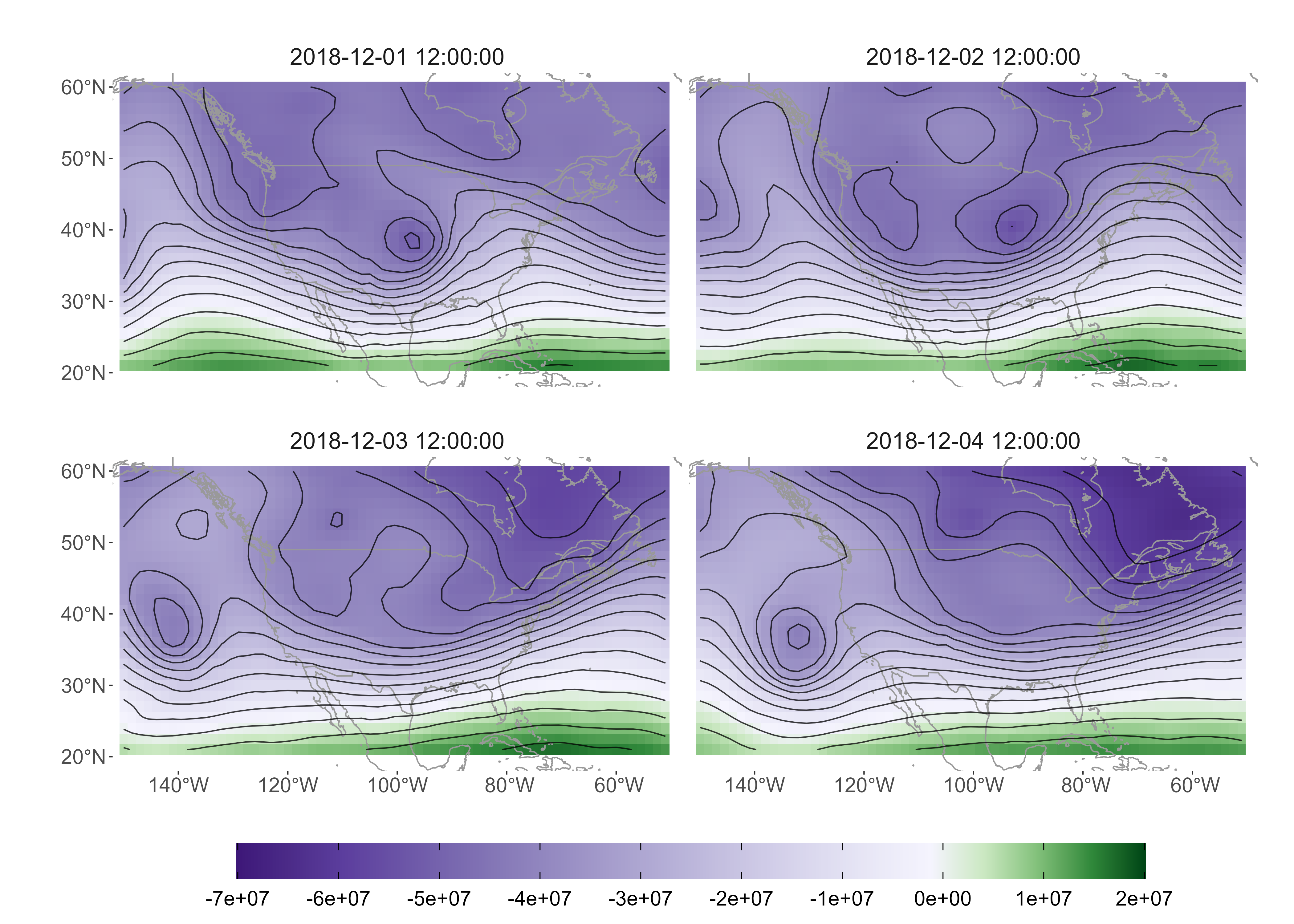
Here, we use hourly data generated using Copernicus Atmosphere Monitoring Service information (2022)11 1 https://cds.climate.copernicus.eu/cdsapp#!/dataset/10.24381/cds.bd0915c6?tab=overview of relative geopotential height at 500-hPA. Data are collected hourly from December 1st to December 31, 2018 over the spatial domain at a resolution of 1.5 degrees (see Figure 5 for example plots), resulting in space-time locations. We compute the streamfunction from the geopotential height and use this as the observed data for the discovery. We also compute the derivative of the Coriolis parameter in the latitudinal direction, , and use it as a covariate in the model (i.e., from (3.7)).
We specify our model with and define the feature library as
Posterior estimates for the recovered equation are shown in Table 7, where only terms with a posterior inclusion probability greater than 50% were kept. While we do not know the true equation in this case (because the barotropic vorticity equation is only an approximation of the dynamics in the atmosphere), we see the discovered equation closely resembles the hypothesized BVE given in (6.1).
Although the sign for each discovered term aligns with the sign in the BVE, we note that the coefficient values are different from the hypothesized equation and the planetary vorticity term () is not significant. There are several reasons why this is likely the case and not surprising. First, it is possible that this particular time period is not barotropic (e.g., baroclinic), which would require library terms our current framework cannot accommodate (e.g., flow in the vertical direction, density, temperature). Such transient changes from barotropic to baroclinic flow regimes are common in the upper-level atmospheric flow. The lack of significance of the planetary vorticity term is also interesting. Recall that the meridional velocity is related to the gradient of streamfunction in the meridional direction, so this term can be alternatively written . Thus, if the flow is primarily zonal (east-west), the north-south flow component () is quite small and this term may not be important for a particular time period. Indeed, visual examination of the data suggests that the flow is dominated by zonal flow and this is further confirmed seeing that the magnitude of the planetary vorticity term in the BVE is an order of magnitude smaller compared to the relative vorticity terms. Yet, the planetary vorticity term is still important to the advection of relative vorticity because of the Coriolis effect on the flow, resulting in the term being identified as important (if not significant). We also note that the planetary vorticity term in the BVE is important for supporting so-called Rossby waves (slowly moving westward propagating synoptic-scale waves) in the upper level flow. Yet, the time period and spatial extent of the data considered here are likely not sufficient to capture the full spatial and temporal scale of Rossby waves (Holton and Hakim, 2012, e.g.,). Thus, it is somewhat remarkable that the dynamic discovery methodology was still able to infer realistic properties of the system of interest that generally align with the theoretical system. To the best of our knowledge, this is the first time that data-driven discovery methods have been applied to real-world atmospheric data and have identified physically plausible features.
| Statistic | Discovered Equation |
|---|---|
| Mean | |
| Lower HPD | |
| Upper HPD |
7 Conclusion
We have proposed a data-driven approach for learning complex non-linear spatio-temporal dynamic equations that is robust to measurement noise and missing data. Our approach uses a Bayesian hierarchical model where the dynamic equation is embedded in the latent process enabling the discovery of dynamic equations within the statistical framework. Additionally, the model provides probabilistic estimates of inclusion for each component of the feature library and estimates of uncertainty for the recovered parameters, giving a deeper understanding to the dynamic system. This all stems from the expansion of the dynamic process in terms of basis functions, bypassing the need for numerical differentiation and enabling the estimate of the derivatives within a probabilistic framework.
Improvements to the current framework should focus on the specification of the feature library and the selection prior. A feature library that is uninhibited by the users choice (i.e., the model could generate library terms) would remove user bias. This is akin to what has been proposed with symbolic regression. Also, a different choice in selection prior for the coefficients, perhaps one that also penalizes model complexity, has the potential to improve selection performance. While there are a variety of selection priors in the literature, a prior directed towards this problem will provide noticeable improvement on the identification of the system.
From the application perspective, the promising and intriguing results from the BVE example suggest further investigation. In particular, it would be informative to consider larger spatial domains (hemispheric) and temporal time periods (many months) to determine if the presence of Rossby waves are sufficient to lead to a significant planetary vorticity term. This also suggests experiments with numerical simulation models that can easily be controlled to exhibit barotropic or baroclinic flow. Such models will allow us to investigate the effects of the flow regime on the ability to detect realistic dynamics.
References
- Bateman, (1915) Bateman, H. (1915). Some recent researches on the motion of fluids. Monthly Weather Review, 43(4):163–170.
- Berliner, (1996) Berliner, L. M. (1996). Hierarchical Bayesian time series models. In Maximum Entropy and Bayesian Methods, pages 15–22. Springer Netherlands, Dordrecht.
- Berliner, (2003) Berliner, L. M. (2003). Physical-statistical modeling in geophysics. Journal of Geophysical Research: Atmospheres, 108(D24).
- Bezanson et al., (2017) Bezanson, J., Edelman, A., Karpinski, S., and Shah, V. B. (2017). Julia: A fresh approach to numerical computing. SIAM Review, 59(1):65–98.
- Bolker and Grenfell, (1995) Bolker, B. and Grenfell, B. (1995). Space, persistence and dynamics of measles epidemics. Philosophical Transactions of the Royal Society of London. Series B: Biological Sciences, 348(1325):309–320.
- Bongard and Lipson, (2007) Bongard, J. and Lipson, H. (2007). Automated reverse engineering of nonlinear dynamical systems. Proceedings of the National Academy of Sciences, 104(24):9943–9948.
- Boninsegna et al., (2018) Boninsegna, L., Nüske, F., and Clementi, C. (2018). Sparse learning of stochastic dynamical equations. The Journal of Chemical Physics, 148(24):241723.
- Both et al., (2021) Both, G.-J., Choudhury, S., Sens, P., and Kusters, R. (2021). DeepMoD: Deep learning for model discovery in noisy data. Journal of Computational Physics, 428(1):109985.
- Brunton et al., (2016) Brunton, S. L., Proctor, J. L., and Kutz, J. N. (2016). Discovering governing equations from data by sparse identification of nonlinear dynamical systems. Proceedings of the National Academy of Sciences, 113(15):3932–3937.
- Burgers, (1948) Burgers, J. (1948). A mathematical model illustrating the theory of turbulence. In Advances in Applied Mechanics, volume 1, pages 171–199. Elsevier.
- Carvalho et al., (2010) Carvalho, C. M., Polson, N. G., and Scott, J. G. (2010). The horseshoe estimator for sparse signals. Biometrika, 97(2):465–480.
- Champion et al., (2020) Champion, K., Zheng, P., Aravkin, A. Y., Brunton, S. L., and Kutz, J. N. (2020). A unified sparse optimization framework to learn parsimonious physics-informed models from data. IEEE Access, 8:169259–169271.
- Charney et al., (1950) Charney, J. G., FjÖrtoft, R., and Neumann, J. V. (1950). Numerical integration of the barotropic vorticity equation. Tellus, 2(4):237–254.
- Cressie and Wikle, (2011) Cressie, N. A. C. and Wikle, C. K. (2011). Statistics for spatio-temporal data. John Wiley & Sons.
- de Silva et al., (2020) de Silva, B., Champion, K., Quade, M., Loiseau, J.-C., Kutz, J., and Brunton, S. (2020). PySINDy: A Python package for the sparse identification of nonlinear dynamical systems from data. Journal of Open Source Software, 5(49):2104.
- Fasel et al., (2021) Fasel, U., Kutz, J. N., Brunton, B. W., and Brunton, S. L. (2021). Ensemble-SINDy: Robust sparse model discovery in the low-data, high-noise limit, with active learning and control. ArXiv, pages 1–18.
- Gelman, (2006) Gelman, A. (2006). Prior distributions for variance parameters in hierarchical models (comment on article by Browne and Draper). Bayesian Analysis, 1(3):515 – 534.
- George et al., (1993) George, E. I., McCulloch, R. E., George, E. I., and McCulloch, R. E. (1993). Variable selection via Gibbs sampling. Journal of the American Statistical Association, 88(423):881–889.
- Hastings, (1996) Hastings, A. (1996). Models of spatial spread: Is the theory complete? Ecology, 77(6):1675–1679.
- Higham et al., (2016) Higham, N. J., Dennis, M. R., Glendinning, P., Martin, P. A., Santosa, F., and Tanner, J. (2016). The Princeton companion to applied mathematics. Princeton University Press.
- Hirsh et al., (2021) Hirsh, S. M., Barajas-Solano, D. A., and Kutz, J. N. (2021). Sparsifying priors for Bayesian uncertainty quantification in model discovery. ArXiv, pages 1–22.
- Holton and Hakim, (2012) Holton, J. R. and Hakim, G. J. (2012). An introduction to dynamic meteorology. Academic Press, 5 edition.
- Hooten and Wikle, (2008) Hooten, M. B. and Wikle, C. K. (2008). A hierarchical Bayesian non-linear spatio-temporal model for the spread of invasive species with application to the Eurasian Collared-Dove. Environmental and Ecological Statistics, 15(1):59–70.
- Huang and Wand, (2013) Huang, A. and Wand, M. P. (2013). Simple marginally noninformative prior distributions for covariance matrices. Bayesian Analysis, 8(2):439–452.
- Kolda, (2006) Kolda, T. (2006). Multilinear operators for higher-order decompositions. Technical Report April, Sandia National Laboratories (SNL), Albuquerque, NM, and Livermore, CA (United States).
- Kolda and Bader, (2009) Kolda, T. G. and Bader, B. W. (2009). Tensor decompositions and applications. SIAM Review, 51(3):455–500.
- Kühnert et al., (2014) Kühnert, D., Stadler, T., Vaughan, T. G., and Drummond, A. J. (2014). Simultaneous reconstruction of evolutionary history and epidemiological dynamics from viral sequences with the birth–death SIR model. Journal of The Royal Society Interface, 11(94):20131106.
- Kuhnert, (2017) Kuhnert, P. M. (2017). Physical-statistical modeling. In Wiley StatsRef: Statistics Reference Online, pages 1–5. Wiley.
- Li and Lin, (2010) Li, Q. and Lin, N. (2010). The Bayesian elastic net. Bayesian Analysis, 5(1):151–170.
- Liu et al., (2019) Liu, H., Ye, Y., Wei, Y., Ma, W., Ma, M., and Zhang, K. (2019). Pattern formation in a reaction-diffusion predator-prey model with weak allee effect and delay. Complexity, 2019(1):1–14.
- Long et al., (2019) Long, Z., Lu, Y., and Dong, B. (2019). PDE-Net 2.0: Learning PDEs from data with a numeric-symbolic hybrid deep network. Journal of Computational Physics, 399:108925.
- Long et al., (2017) Long, Z., Lu, Y., Ma, X., and Dong, B. (2017). PDE-Net: Learning PDEs from data. 35th International Conference on Machine Learning, ICML 2018, 7:5067–5078.
- Malsiner-Walli and Wagner, (2016) Malsiner-Walli, G. and Wagner, H. (2016). Comparing spike and slab priors for Bayesian variable selection. Austrian Journal of Statistics, 40(4).
- Mandt et al., (2016) Mandt, S., Hoffman, M., and Blei, D. (2016). A variational analysis of stochastic gradient algorithms. Proceedings of The 33rd International Conference on Machine Learning, 48:354–363.
- Mangal et al., (2008) Mangal, T. D., Paterson, S., and Fenton, A. (2008). Predicting the impact of long-term temperature changes on the epidemiology and control of Schistosomiasis: A mechanistic model. PLoS ONE, 3(1):e1438.
- Milliff et al., (2011) Milliff, R. F., Bonazzi, A., Wikle, C. K., Pinardi, N., and Berliner, L. M. (2011). Ocean ensemble forecasting. Part I: Ensemble Mediterranean winds from a Bayesian hierarchical model. Quarterly Journal of the Royal Meteorological Society, 137(657):858–878.
- Mitchell and Beauchamp, (1988) Mitchell, T. J. and Beauchamp, J. J. (1988). Bayesian variable selection in linear regression. Journal of the American Statistical Association, 83(404):1023.
- Niven et al., (2020) Niven, R., Mohammad-Djafari, A., Cordier, L., Abel, M., and Quade, M. (2020). Bayesian identification of dynamical systems. Proceedings, 33(1):33.
- North et al., (2022) North, J. S., Wikle, C. K., and Schliep, E. M. (2022). A Bayesian approach for data-driven dynamic equation discovery. Journal of Agricultural, Biological, and Environmental Statistics, 1(1):1–28.
- Park and Casella, (2008) Park, T. and Casella, G. (2008). The Bayesian lasso. Journal of the American Statistical Association, 103(482):681–686.
- Rackauckas and Nie, (2017) Rackauckas, C. and Nie, Q. (2017). DifferentialEquations.jl – A performant and feature-rich ecosystem for solving differential equations in Julia. Journal of Open Research Software, 5(1):15.
- Raissi and Karniadakis, (2018) Raissi, M. and Karniadakis, G. E. (2018). Hidden physics models: Machine learning of nonlinear partial differential equations. Journal of Computational Physics, 357:125–141.
- Raissi et al., (2017) Raissi, M., Perdikaris, P., and Karniadakis, G. E. (2017). Physics informed deep learning (Part I): Data-driven solutions of nonlinear partial differential equations. arXiv preprint arXiv:1711.10561, Part I:1–22.
- Raissi et al., (2020) Raissi, M., Yazdani, A., and Karniadakis, G. E. (2020). Hidden fluid mechanics: Learning velocity and pressure fields from flow visualizations. Science, 367(6481):1026–1030.
- Ramsay and Silverman, (2005) Ramsay, J. O. and Silverman, B. W. (2005). Functional data analysis. Springer Series in Statistics. Springer New York, New York, NY.
- Reichstein et al., (2019) Reichstein, M., Camps-Valls, G., Stevens, B., Jung, M., Denzler, J., Carvalhais, N., and Prabhat (2019). Deep learning and process understanding for data-driven Earth system science. Nature, 566(7743):195–204.
- Revels et al., (2016) Revels, J., Lubin, M., and Papamarkou, T. (2016). Forward-mode automatic differentiation in Julia. ArXiv.
- Ročková and George, (2014) Ročková, V. and George, E. I. (2014). Negotiating multicollinearity with spike-and-slab priors. METRON, 72(2):217–229.
- Royle et al., (1999) Royle, J. A., Berliner, L. M., Wikle, C. K., and Milliff, R. (1999). A Hierarchical spatial model for constructing wind fields from scatterometer data in the Labrador Sea. In Case Studies in Bayesian Statistics., pages 367–382. Springer, New York, NY.
- (50) Rudy, S., Alla, A., Brunton, S. L., and Kutz, J. N. (2019a). Data-driven identification of parametric partial differential equations. SIAM Journal on Applied Dynamical Systems, 18(2):643–660.
- Rudy et al., (2017) Rudy, S. H., Brunton, S. L., Proctor, J. L., and Kutz, J. N. (2017). Data-driven discovery of partial differential equations. Science Advances, 3(4):e1602614.
- (52) Rudy, S. H., Nathan Kutz, J., and Brunton, S. L. (2019b). Deep learning of dynamics and signal-noise decomposition with time-stepping constraints. Journal of Computational Physics, 396:483–506.
- Schaeffer, (2017) Schaeffer, H. (2017). Learning partial differential equations via data discovery and sparse optimization. Proceedings of the Royal Society A: Mathematical, Physical and Engineering Sciences, 473(2197):20160446.
- Schmidt and Lipson, (2009) Schmidt, M. and Lipson, H. (2009). Distilling free-form natural laws from experimental data. Science, 324(5923):81–85.
- Sun et al., (2019) Sun, Y., Zhang, L., and Schaeffer, H. (2019). NeuPDE: Neural network based ordinary and partial differential equations for modeling time-dependent data. arXiv preprint arXiv:1908.03190, 107(2016):352–372.
- Tibshirani, (1996) Tibshirani, R. (1996). Regression shrinkage and selection via the lasso. Journal of the Royal Statistical Society: Series B (Methodological), 58(1):267–288.
- Tsitouras, (2011) Tsitouras, C. (2011). Runge–Kutta pairs of order 5(4) satisfying only the first column simplifying assumption. Computers & Mathematics with Applications, 62(2):770–775.
- Tucker, (1966) Tucker, L. R. (1966). Some mathematical notes on three-mode factor analysis. Psychometrika, 31(3):279–311.
- Wang et al., (2016) Wang, J. L., Chiou, J. M., and Müller, H. G. (2016). Functional data analysis. Annual Review of Statistics and Its Application, 3:257–295.
- White and Majdalani, (2006) White, F. M. and Majdalani, J. (2006). Viscous fluid flow. McGraw-Hill New York, 3 edition.
- Wikle, (2003) Wikle, C. K. (2003). Hierarchical Bayesian models for predicting the spread of ecological processes. Ecology, 84(6):1382–1394.
- Wikle et al., (2001) Wikle, C. K., Milliff, R. F., Nychka, D., and Berliner, L. M. (2001). Spatiotemporal hierarchical Bayesian modeling: Tropical ocean surface winds. Journal of the American Statistical Association, 96(454):382–397.
- Wu and Xiu, (2020) Wu, K. and Xiu, D. (2020). Data-driven deep learning of partial differential equations in modal space. Journal of Computational Physics, 408:109307.
- Xu et al., (2019) Xu, H., Chang, H., and Zhang, D. (2019). DL-PDE: Deep-learning based data-driven discovery of partial differential equations from discrete and noisy data. Communications in Computational Physics, 29(3):698–728.
- Xu et al., (2020) Xu, H., Chang, H., and Zhang, D. (2020). DLGA-PDE: Discovery of PDEs with incomplete candidate library via combination of deep learning and genetic algorithm. Journal of Computational Physics, 418:109584.
- Xu et al., (2021) Xu, H., Zhang, D., and Zeng, J. (2021). Deep-learning of parametric partial differential equations from sparse and noisy data. Physics of Fluids, 33(3):037132.
- Yang et al., (2019) Yang, H.-C., Hu, G., and Chen, M.-H. (2019). Bayesian variable selection for pareto regression models with latent multivariate log gamma process with applications to earthquake magnitudes. Geosciences, 9(4):169.
- Yang et al., (2020) Yang, Y., Aziz Bhouri, M., and Perdikaris, P. (2020). Bayesian differential programming for robust systems identification under uncertainty. Proceedings of the Royal Society A: Mathematical, Physical and Engineering Sciences, 476(2243):20200290.
- Zellner, (1986) Zellner, A. (1986). On assessing prior distributions and Bayesian regression analysis with g-prior distributions. Bayesian Inference and Decision Techniques, pages 233–243.
- Zhang and Lin, (2018) Zhang, S. and Lin, G. (2018). Robust data-driven discovery of governing physical laws with error bars. Proceedings of the Royal Society A: Mathematical, Physical and Engineering Sciences, 474(2217):20180305.
- Zheng et al., (2019) Zheng, P., Askham, T., Brunton, S. L., Kutz, J. N., and Aravkin, A. Y. (2019). A unified framework for sparse relaxed regularized regression: SR3. IEEE Access, 7:1404–1423.
S Supplementary Material
S.1 Inclusion Probabilities for Spike and Slab
Let the residual sum of squares for the model with the term included be and the model without the term included be . The probability any element is included is given as
where
Denote and solving for the number of observations ,
We then use the value of to inform our subsample size based on , the ratio of the RSSs, and an informed value of . For example, assume such that every parameter has a 50% chance of being included in the model. We would take resulting in . is then chosen by solving the equation under a hypothetical (e.g., or ).
In choosing the value there are a couple things to consider. If the terms in the library are highly correlated, there is likely to be confounding and incorrect variables may have a larger impact on the RSS. This issue is detected using the condition number of the correlation matrix (e.g., where is the normalized version of ), where a large condition number (e.g., greater than 1000) indicates multicollinearity. Under the scenario where the condition number is large, should be chosen to be smaller (i.e., 0.9 or 0.95), resulting in a smaller subsampled size. Alternatively, if the variables are less correlated (i.e., condition number smaller than 1000), the impact of an incorrect variable on the RSS will be less. In this case can be chosen to be closer to one (e.g., 0.99 or 0.999), resulting in a larger subsample size. When fitting the model, the parameter will be estimated and will (likely) not be 0.5. However, empirically we have found taking and to solve for works well.
For the simulations, the condition number of the correlation matrix for Burgers’ is approximately 28940, the Heat equation is approximately 1840, and the reaction-diffusion equation is approximately 6510. We chose to be 0.9, 0.99, and 0.95 for Burgers’, the Heat, and the reaction-diffusion equations, respectively. For the real-world example, the condition number of the correlation matrix is approximately 480 and we chose to be 0.99.
A parallel can be drawn between the subsampling and sequential thresholded least squares (Brunton et al., 2016, STLS;) or sequential threshold ridge regression (Rudy et al., 2017, STRidge;). Because the inclusion probability is affected by the subsample size (i.e., reduces the inclusion probability or highly unlikely terms), this is analogous to a probabilistic extension of the thresholding approaches. That is, instead of assigning a hard threshold, where values less than a predetermined value are set to zero, the subsampling approach impacts the probability of a variable being included below a certain threshold based on a specified .
S.2 Sampling Algorithm
To simplify notation, denote and . At time and location , the full model is
For iteration do:
- 1.
Obtain minibatch .
- 2.
Update : Denote as the design matrix consisting only of columns of corresponding to non-zero effects, , and . Let , and correspond to and , and correspond to . Sample each element of of the indicator vector from
where .
- 3.
Update : For , sample
- 4.
Update : For , set is . For non-zero elements, sample
- 5.
Update : For , sample
- 6.
Update : For , sample
and
- 7.
Update : Use (4.1) to update .
S.3 Proofs of Propositions
Proposition 1. The mode-3 decomposition of where in space and time at location and time is
where is a matrix of basis coefficients, is a length- vector of spatial basis functions, is a length- vector of temporal basis functions, and is a matrix of component basis functions.
Proof of Proposition 1. For the LHS, is the mode-3 matricization of (see Kolda, 2006, for a proof of this property). For the RHS, from the property of the n-mode product, , where is the mode-3 matricization of . The arguments of , namely , are represented using their basis expansion, resulting in depending on and any derivatives of and needed for the library. The value at a specific space-time location is determined from the th and th column of and , respectively. The last term on the RHS, , is a the mode-3 matricization of the uncertainty tensor , where each space-time location has the same variance-covariance matrix .
Proposition 2. Let be a linear differential operator. The basis formulation of a PDE with a space-time response is
Proof of Proposition 2. Let be a function of the tensor of the continuous process observed at discrete space-time locations. Decomposing in terms of spatial, temporal, and component basis functions, . From Proposition 1, the mode-3 basis decomposition of is . By linearity of and properties of the Kronecker product,
The function at location and time is
S.4 Extra Tables
| Noise | Missing Data | First Term | Probability | Second Term | Probability |
|---|---|---|---|---|---|
| 0% | 0% | 0.193 | 0.139 | ||
| 2% | 0% | 0.222 | 0.145 | ||
| 5% | 0% | 0.235 | 0.164 | ||
| 2% | 5% | 0.229 | 0.150 |
| Noise | First Term | Probability | Second Term | Probability |
|---|---|---|---|---|
| 0% | 0.050 | 0.037 | ||
| 2% | 0.015 | 0.013 | ||
| 5% | 0.030 | 0.010 |
| Noise | Component | First Term | Probability | Second Term | Probability |
|---|---|---|---|---|---|
| 0% | Prey | 0.040 | 0.039 | ||
| 0% | Predator | 0.057 | 0.036 | ||
| 2% | Prey | 0.022 | 0.020 | ||
| 2% | Predator | 0.020 | 0.019 | ||
| 5% | Prey | 0.029 | 0.027 | ||
| 5% | Predator | 0.024 | 0.023 |
Acknowledgments
The authors would like to acknowledge Dr. Ralph Milliff for comments on an early draft and for helpful discussions concerning the results from the barotropic vorticity example. This research was partially supported by the U.S. National Science Foundation (NSF) grant SES-1853096 and the U.S. Geological Survey Midwest Climate Adaptation Science Center (CASC) grant No.G20AC00096.