Mortaring for linear elasticity using mixed and stabilized finite elements
Abstract
The purpose of this work is to study mortar methods for linear elasticity using standard low order finite element spaces. Based on residual stabilization, we introduce a stabilized mortar method for linear elasticity and compare it to the unstabilized mixed mortar method. For simplicity, both methods use a Lagrange multiplier defined on a trace mesh inherited from one side of the interface only. We derive a quasi-optimality estimate for the stabilized method and present the stability criteria of the mixed approximation. Our numerical results demonstrate the stability and the convergence of the methods for tie contact problems. Moreover, the results show that the mixed method can be successfully extended to three dimensional problems.
1 Introduction
Mortaring via Lagrange multipliers is also a prototype of elastic contact problems besides its use in domain decomposition. Consider, for example, a linear elastic body , , with the displacement field and body loading . In the absence of other external forces, the principle of virtual work reads as follows:
where is the infinitesimal strain tensor, is the linear elastic stress tensor corresponding to the fourth-order constitutive tensor , and is the space of kinematically admissible displacement fields. Suppose now that is split into two parts and with the displacements and , respectively. The continuity across the interface can be enforced using a vectorial Lagrange multiplier field , , through the saddle point formulation
| (1) |
where is the trace space of on the interface . In contact mechanics, the linear saddle point formulation (1) corresponds to a single contact iteration with zero initial gap between the bodies and . In fact, the stability results carry over to the variational inequality formulations. Formulation (1) is sometimes referred to as tie contact problem.
In principle, the Lagrange multiplier formulation can accommodate nonmatching computational meshes and even different finite element spaces over , and, thus, can be made quite generic with respect to the discretization of parts and . However, it is well known [1] that saddle point system (1) is stable only if a certain compatibility criterion, the Babuška–Brezzi condition, holds for the finite element discretizations of and . The lack of stability can have various consequences from reduction in the asymptotic convergence rate to a singular linear system. Moreover, the instability may manifest itself only for specific mesh configurations. In dealing with mortar finite element methods, this has led to the development of special finite element techniques aiming at proving stability independently of the finite element mesh. These techniques include enriching the displacement field with bubble degrees-of-freedom [2, 3], special biorthogonal finite element bases for the Lagrange multiplier [4, 5, 6], local modification of basis functions at the interface [7, 8, 9], or modification of the bilinear form using additional stabilizing terms [10, 11, 12, 13].
Based on the abundance of literature on such special stabilization techniques, it could be easily inferred that they are absolutely necessary for successful approximation of tie contact problems. However, many existing finite element solvers implement piecewise-linear finite elements and, therefore, it is natural to consider also standard finite elements for the mixed variational formulation and analyze their stability criteria. The pair , i.e. piecewise-linear displacement and piecewise-constant Lagrange multiplier, is not stable, cf. [5]. However, continuous piecewise-linear elements for both the displacement and the Lagrange multiplier can be made stable by special modifications of the basis functions at Dirichlet boundaries or at interface junctions between three or more subdomains, cf. [9, 8, 2]. We argue that in contact mechanics one is less likely to encounter such configurations and proceed with the study of the unmodified pair, assuming that the bodies are not fixed right next to the contact interface.
The purpose of this work is to study the discretization of the saddle point problem (1) using mixed and stabilized finite element methods and investigate the stability and the convergence of the methods. In the past, residual-based Barbosa–Hughes stabilization [14] has been applied to interface problems, e.g., for the Poisson equation [15] as well as frictionless [16] and frictional contact [12]. Here we introduce, to our knowledge for the first time, residual stabilized mortar method for tie contact or, equivalently, domain decomposition in linear elasticity. The method is proven stable for any -conforming finite element spaces which is shown to lead to a quasi-optimality error estimate. Next we consider a mixed method using a continuous Lagrange multiplier and present criteria for the stability of the lowest order method under which we are able to prove the Babuška–Brezzi condition. For additional verification, we present novel numerical results comparing the behavior of the mixed and stabilized methods under uniform refinements, and unique three-dimensional results using an implementation of the mixed method in Elmer [17], a suite of open source finite element solvers for multiphysical problems.
2 Problem formulation
The boundary is split into the Dirichlet part , the Neumann part , , and the interface between the two domains and . We assume that and are always separated by to avoid using the trace space [18]. Moreover, if and are not separated, then the finite element space associated with the Lagrange multiplier in the mixed formulation requires modification [2].
The strong formulation of the tie contact problem reads as follows:
| (2) |
where
| (3) |
and are the material parameters (Young’s modulus and Poisson ratio). The formulation is complemented with fixed and zero traction boundary conditions
| (4) |
and the interface conditions
| (5) |
guaranteeing the continuity of the traction across the interface .
Let us define the function space and the dual space where is the dimension of the domain and refers to the space of traces of functions in on . In the following, we use the notation and, consequently, . The variational formulation of (2)–(5) then reads as: find satisfying
| (6) |
for every . In (6), denotes the -inner product over the subdomain and is the -duality pairing. Equivalently, we write (6) as: find satisfying
| (7) |
where the bilinear form and the linear form are defined as
and denotes the jump of the displacement across the interface . Existence and uniqueness of (7) are standard and follows the steps laid out in [1].
3 Stabilized finite element method
Let be a computational mesh of the domain , , with the mesh parameter and be the set of edges/facets of on the interface . To introduce the stabilized finite element method, we define the discrete spaces
where and are the polynomial degrees. We stress that the space is defined using the edges/facets of only.
Let be such that , and let be a stabilization parameter. The discrete bilinear form , defined as
| (8) |
is continuous and stable in the following mesh-dependent norm (see Theorem 1 below):
| (9) |
Note that (8) is stabilized using the residual of (5). In (9), the norm for the displacement is given by the strain energy:
The stabilized finite element formulation now reads as follows: find satisfying
The stability of the formulation is proved in the following theorem.
Theorem 1.
For small enough and any there exists , independent of , such that
Proof.
Remark 1.
From the proof of Theorem 1, it is obvious that the result holds for any -conforming Lagrange multiplier space, continuous or discontinuous. One may even use non-local functions to define a global spectral basis. This idea has been used, e.g., in Hansbo et al. [20, 15] to simplify the implementation and circumvent the need for a conforming integration mesh. Moreover, it is possible to eliminate a discontinuous, piecewise polynomial Lagrange multiplier locally on each element to arrive at a positive definite Nitsche-type method [21, 11, 19].
As a consequence of Theorem 1, we have the following quasi-optimality estimate:
Theorem 2.
Suppose . There exists such that
Proof.
Discrete stability (Theorem 1), the orthogonality result
and continuity of , imply that
Dividing both sides by and using the triangle inequality leads to the proof. ∎
4 Mixed finite element method
Let us next consider a mixed method using a continuous Lagrange multiplier, i.e. the spaces
| (10) | ||||
where . This approach is mentioned in the early work of Pitkäranta [22] where it is noted that the discrete stability holds if the space of Lagrange multipliers is a subset of the trace space of . However, the stability may not, in general, be uniform in without additional restrictions on the finite element mesh.
The discrete mixed formulation reads as follows: find satisfying
The Babuška–Brezzi condition, guaranteeing stability is written as: there exists , independent of , such that
| (11) |
Here we establish the uniform stability for the mixed method using the mesh-dependent norm in and the following auxiliary result [21].
Lemma 1.
Lemma 1 can be proven independently of the finite element spaces for any shape regular mesh families using the stability of the continuous problem and Clément interpolation, cf. [21]. The following assumption on the finite element mesh is sufficient for stability in the mesh-dependent norm, see [23] for a discussion on similar estimates with graded meshes.
Assumption 1.
The -projection satisfies
Theorem 3.
Proof.
Let , where , be the extension of a piecewise linear function on to defined via the finite element basis so that the nodes outside of the interface have value zero. For such an extension it holds [24]
| (13) |
From the definition of the -projection, choosing , it follows that
| (14) |
Using Korn’s inequality, property (13) and Assumption 1, we obtain
| (15) | ||||
Remark 3.
5 Numerical experiments
In this section, we perform experiments using both methods and different polynomial orders. We refer to the method using polynomial order for the displacement and for the continuous Lagrange multiplier as mixed method. The two-dimensional examples are implemented using scikit-fem [26] and visualized using matplotlib [27] whereas the three-dimensional examples are implemented using the finite element software Elmer [17] and visualized using Paraview [28]. In all examples the material parameters are taken to be and in both bodies. The source code and problem definition files for reproducing the numerical examples are available in [29].
5.1 Square against square, unstable example
For completeness, we first demonstrate the instability of mixed method and how stabilization recovers the expected rate of convergence. The domain is
The interface is
while the boundaries are
and the essential boundary conditions are given by
First, we demonstrate that the instability of mixed method with a piecewise constant Lagrange multiplier is clearly visible when using matching vertices. The initial meshes are given in Figure 1. The Lagrange multipliers are visualized in Figure 2 from which it becomes clear that the tangential Lagrange multiplier does not properly represent the true solution. This is further exemplified in Figure 3 (left) where we observe that the convergence rate of the Lagrange multiplier is seriously affected by the lack of stabilization.
For the stabilized method, we observe superconvergence of the Lagrange multiplier with the error of the order – instead of as suggested by the linear approximation of the primal variable. The reference solution was calculated using a stabilized method and a very fine mesh.
5.2 Square against square, methods
In order to demonstrate the stability of the mixed method, we solve the same problem as above using both the mixed method and its stabilized counterpart using a continuous Lagrange multiplier. A nonmatching mesh is used to demonstrate the approach in the case of general meshes. The convergence rates are in Figure 3 (right) and the Lagrange multipliers are visualized in Figure 5. As a conclusion, both methods give essentially the same results. As above, we observe superconvergence of the Lagrange multiplier with the error of order .
5.3 Three-dimensional examples
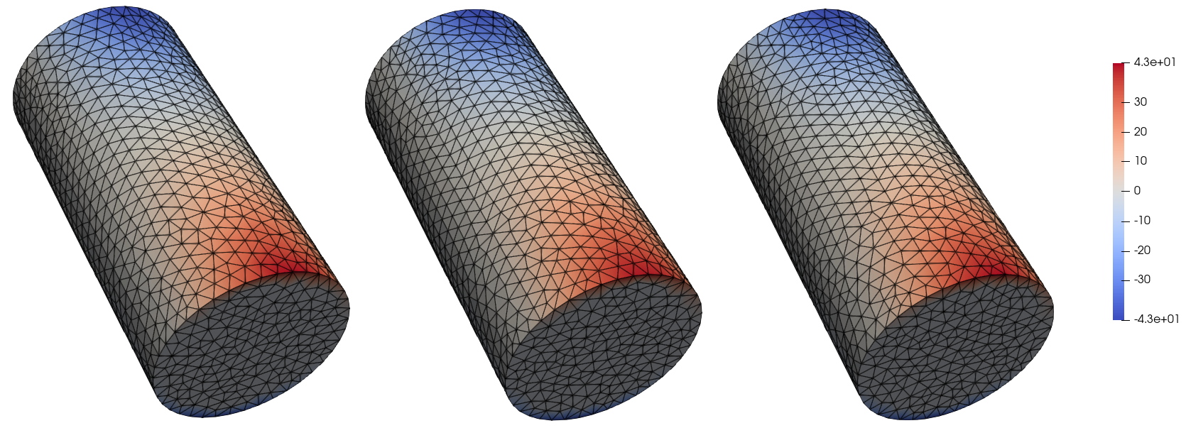
The mixed method is implemented in Elmer [17] for three-dimensional geometry. We first present an example where a cylinder with the radius and height of 0.5 and 1, respectively, is pushed against a cube with side length of 1, see Figure 6. The external force is introduced through inhomogeneous Dirichlet boundary condition, i.e. the bottom surface of the block is fixed whereas the top surface of the cylinder is forced downwards 0.1 units. Consequently, the exact solution is independent of the cylinder’s axial rotation and the discrete problem can be solved using several angles to observe how the orientation of elements affects the contact force.
The cylinder is discretized using linear tetrahedral elements in Gmsh [30] and the block is discretized using trilinear hexahedral tensor product grid. The normal and tangential components of the contact force are given for three different values of cylinder’s axial rotation (0, and ) in Figures 7 and 8. All rotation angles lead to practically identical normal and tangential contact forces which suggests that the method is robust with respect to the shape and the orientation of the elements at the contact interface.
The second three-dimensional example concerns a more complicated geometry with a cylindrical shaft cutting through a block. The cylinder has radius and height 1, and the block is a cube with side length of 1, see Figure 9. The block is squeezed 0.1 units using a similar boundary condition as before. The cylinder is rotated around its axis and results are obtained for several angles of rotation. The contact forces are given in Figures 10 and 11 demonstrating once again the independence of the results on the finite element mesh.
The final example is a three-dimensional version of the convergence study in Section 5.2. More precisely, a cubical block with side length of 1 is pushed downward against another block with same horizontal dimensions and of height 0.5. As we do not possess a sufficiently accurate reference solution, we compute the strain energy at different mesh refinement levels and visualize its change as a function of the mesh parameter, see Figure 14 where a linear rate is demonstrated. The corresponding contact forces are shown in Figures 12 and 13.
6 Discussion
Mortar finite element methods and tie contact problems are naturally presented in a mixed variational formulation and their discretizations often use special finite element spaces. In this paper, we have presented two finite element formulations, mixed and stabilized, for the approximation of the elastic tie contact problem. Both use standard finite element spaces and are stable for continuous elements, the mixed method under certain mild assumptions on the boundary conditions and the finite element mesh, and lead to similar numerical results. The mixed method has been implemented for general two- and three-dimensional contact problems in Elmer [17].
Acknowledgements
The work was supported by the Academy of Finland (Decisions 324611 and 338341) and the Portuguese government through FCT (Fundação para a Ciência e a Tecnologia), I.P., under the projects PTDC/MAT-PUR/28686/2017 and UIDB/04459/2020.




References
- [1] I. Babuška, The finite element method with Lagrangian multipliers, Numerische Mathematik 20 (3) (1973) 179–192.
- [2] P. Hauret, M. Ortiz, BV estimates for mortar methods in linear elasticity, Computer Methods in Applied Mechanics and Engineering 195 (37-40) (2006) 4783–4793.
- [3] P. Hauret, P. Le Tallec, A discontinuous stabilized mortar method for general 3d elastic problems, Computer Methods in Applied Mechanics and Engineering 196 (49-52) (2007) 4881–4900.
- [4] B. I. Wohlmuth, A mortar finite element method using dual spaces for the Lagrange multiplier, SIAM Journal on Numerical Analysis 38 (3) (2000) 989–1012.
- [5] B. Wohlmuth, Variationally consistent discretization schemes and numerical algorithms for contact problems, Acta Numerica 20 (2011) 569–734.
- [6] A. Fritz, S. Hüeber, B. I. Wohlmuth, A comparison of mortar and Nitsche techniques for linear elasticity, Calcolo 41 (3) (2004) 115–137.
- [7] C. Bernardi, Y. Maday, A. T. Patera, Domain decomposition by the mortar element method, in: Asymptotic and numerical methods for partial differential equations with critical parameters, Springer, 1993, pp. 269–286.
- [8] F. B. Belgacem, P. Hild, P. Laborde, The mortar finite element method for contact problems, Mathematical and Computer Modelling 28 (4-8) (1998) 263–271.
- [9] F. B. Belgacem, The mortar finite element method with Lagrange multipliers, Numerische Mathematik 84 (2) (1999) 173–197.
- [10] F. Liu, R. I. Borja, Stabilized low-order finite elements for frictional contact with the extended finite element method, Computer Methods in Applied Mechanics and Engineering 199 (37-40) (2010) 2456–2471.
- [11] T. Gustafsson, R. Stenberg, J. Videman, Error analysis of Nitsche’s mortar method, Numerische Mathematik 142 (4) (2019) 973–994.
- [12] T. Gustafsson, J. Videman, Stabilized finite elements for Tresca friction problem, ESAIM: Mathematical Modelling and Numerical Analysis 56 (4) (2022) 1307–1326.
- [13] P. Heintz, P. Hansbo, Stabilized Lagrange multiplier methods for bilateral elastic contact with friction, Computer Methods in Applied Mechanics and Engineering 195 (33-36) (2006) 4323–4333.
- [14] H. J. Barbosa, T. J. Hughes, The finite element method with Lagrange multipliers on the boundary: circumventing the Babuška-Brezzi condition, Computer Methods in Applied Mechanics and Engineering 85 (1) (1991) 109–128.
- [15] P. Hansbo, C. Lovadina, I. Perugia, G. Sangalli, A Lagrange multiplier method for the finite element solution of elliptic interface problems using non-matching meshes, Numerische Mathematik 100 (1) (2005) 91–115.
- [16] P. Hansbo, A. Rashid, K. Salomonsson, Least-squares stabilized augmented Lagrangian multiplier method for elastic contact, Finite Elements in Analysis and Design 116 (2016) 32–37.
- [17] M. Malinen, P. Råback, Elmer finite element solver for multiphysics and multiscale problems, in: Multiscale Modelling Methods for Applications in Materials Science, Vol. 19, Schriften des Forschungszentrums Jülich, IAS Series, Germany, 2013, pp. 101–113.
- [18] L. Tartar, An introduction to Sobolev spaces and interpolation spaces, Vol. 3, Springer Science & Business Media, 2007.
- [19] T. Gustafsson, R. Stenberg, J. Videman, On Nitsche’s method for elastic contact problems, SIAM Journal on Scientific Computing 42 (2) (2020) B425–B446.
- [20] P. Hansbo, Nitsche’s method for interface problems in computational mechanics, GAMM-Mitteilungen 28 (2) (2005) 183–206.
- [21] T. Gustafsson, R. Stenberg, J. Videman, Mixed and stabilized finite element methods for the obstacle problem, SIAM Journal on Numerical Analysis 55 (6) (2017) 2718–2744.
- [22] J. Pitkäranta, Boundary subspaces for the finite element method with Lagrange multipliers, Numerische Mathematik 33 (3) (1979) 273–289.
- [23] R. E. Bank, H. Yserentant, On the -stability of the -projection onto finite element spaces, Numerische Mathematik 126 (2) (2014) 361–381.
- [24] R. Verfürth, A Posteriori Error Estimation Techniques for Finite Element Methods, Oxford University Press, 2013. doi:10.1093/acprof:oso/9780199679423.001.0001.
- [25] P. Seshaiyer, M. Suri, Uniform convergence results for the mortar finite element method, Mathematics of Computation 69 (230) (2000) 521–546.
- [26] T. Gustafsson, G. D. McBain, scikit-fem: A Python package for finite element assembly, Journal of Open Source Software 5 (52) (2020) 2369. doi:10.21105/joss.02369.
- [27] J. D. Hunter, Matplotlib: A 2d graphics environment, Computing in science & engineering 9 (03) (2007) 90–95.
- [28] J. Ahrens, B. Geveci, C. Law, Paraview: An end-user tool for large data visualization, The visualization handbook 717 (8) (2005).
- [29] T. Gustafsson, P. Råback, Numerical experiments for "Mortaring for linear elasticity using mixed and stabilized finite elements" (Oct. 2022). doi:10.5281/zenodo.7245378.
- [30] C. Geuzaine, J.-F. Remacle, Gmsh: A 3-d finite element mesh generator with built-in pre-and post-processing facilities, International Journal for Numerical Methods in Engineering 79 (11) (2009) 1309–1331.