\doiinfo

10.1007/DOI-NUMBER

Arithmetical Hierarchy of the Besicovitch-Stability of Noisy TilingsVolume: Volume VOL, Number 0NUM, MONTH 2023

Léo Gayral Thanks: This work is an extension upon preliminary results first introduced as an exploratory paper by the first author at Automata 2021˜[9]. Email address: leo.gayral@math.cnrs.fr URL: lgayral.pages.math.cnrs.fr/en and Mathieu Sablik Email address: msablik@math.univ-toulouse.fr URL: math.univ-toulouse.fr/~msablik Address:
Université Toulouse III - Paul Sabatier
Institut de Mathématiques de Toulouse
118, route de Narbonne
F-31062 Toulouse Cedex 9
France

Abstract.

The purpose of this article is to study the algorithmic complexity of the Besicovitch stability of noisy subshifts of finite type, a notion studied in a previous article [10]. First, we exhibit an unstable aperiodic tiling, and then see how it can serve as a building block to implement several reductions from classical undecidable problems on Turing machines. It will follow that the question of stability of subshifts of finite type is undecidable, and the strongest lower bound we obtain in the arithmetical hierarchy is $\Pi_{2}$ -hardness. Lastly, we prove that this decision problem, which requires to quantify over an uncountable set of probability measures, has a $\Pi_{4}$ upper bound.

1. Introduction

Let $\mathcal{A}$ a finite alphabet. A subshift of finite type (SFT), denoted $\Omega_{\mathcal{F}}$ , is a set of $\mathcal{A}$ -colourings of $\mathds{Z}^{d}$ induced by a finite set of forbidden patterns $\mathcal{F}$ which cannot appear in any configuration. One of the main topics of interest in the study of multidimensional SFTs is how a global structure can emerge from local rules. In particular, aperiodic SFTs have been studied by Berger [5], Robinson [25] and Kari [21] among others. One of the most useful properties of the Robinson tiling is that its hierarchical structure leaves room for a relatively easy embedding of Turing machines into it [25, 20].

In the last decade, a lot of studies focused on the links between dynamical properties of SFTs and their algorithmic complexity. The values taken by some dynamical invariants can be characterised as some classes of (non-)computable values: possible entropies [16], or dimension entropies [23], subactions [2, 7, 15], possible periods [18], or some classes of SFTs [31]… These works help to understand the limits of what global behaviours can be enforced by local rules.

These classes of numbers relate to the arithmetical hierarchy of computable sets through the identification between $x\in\mathds{R}$ and the interval $\{q\in\mathds{Q},q<x\}$ . Another way to highlight the complexity of tilings is then to understand the complexity of a decision problem about a dynamical property of the SFTs. These problems are usually undecidable, but may fit into the arithmetical (or analytical) hierarchy. Regarding the arithmetical hierarchy, the Domino problem is $\Pi_{1}$ -complete [25], the conjugacy problem is $\Sigma_{1}$ -complete and the factorisation problem is $\Sigma_{3}$ -complete [19]… Regarding the analytical hierarchy, deciding whether a tiling has a completely positive topological entropy or not is $\Pi_{1}^{1}$ -complete [32], in dimension $d\geq 4$ the aperiodic Domino problem is $\Pi_{1}^{1}$ -complete [13]… To obtain these results, the proofs always involve the embedding of Turing machines into complex (and aperiodic) tilings. This is interesting since few natural problems (not directly related to a computation model) are known to be complete in these hierarchies.

In this article, we study the algorithmic complexity of the Besicovitch-stability of noisy SFTs. In a previous article [10], we introduced this notion of stability using the Besicovitch distance, which quantifies the closeness between measures through the average frequency of differences between their configurations. This framework is a natural bridge from the notion of stability described by Durand, Romashchenko and Shen [7] to ergodic theory, with a viewpoint focusing more on measure theory. The purpose is to understand if SFTs are stable in the presence of noise, if computations can survive if a small proportion of forbidden patterns is permitted. Such studies already exist for cellular automata [12] or Turing machines [1]. A digest of this framework will be introduced in Section 2, followed by a few notions about undecidability and the arithmetical hierarchy.

In the aforementioned article [10], we proved a simple computable criterion (using a word automaton) to decide stability for one-dimensional SFTs. Then, we proved the existence of both stable and unstable SFTs in any dimension, and a specific variant of the Robinson tiling was proven to be stable; before this, the only known stable aperiodic tilings were complex constructions that can be repaired locally, which is not the case for this variant of the Robinson tiling [3, 7, 28]. However, the interface between stable and unstable examples in general was yet to be seen.

In this article, we will prove that a known two-coloured Robinson tiling is unstable in Section 3, and describe a general framework to obtain stability for some quasi-periodic SFTs in Section 4. By iterating upon both the stable and unstable constructions, we will step-by-step craft simulating tilings to show that deciding if a SFT is stable is $\Pi_{1}$ -hard, $\Sigma_{1}$ -hard and finally $\Pi_{2}$ -hard in Section 5.

After this, we will obtain a $\Pi_{4}$ upper bound for stability in Section 6. This bound may be surprising a priori since the definition of stability requires to quantify over uncountable sets (of translational-invariant probability measures). To obtain such a bound we will dig deeper into the technicalities of computable analysis on measures, to rewrite the stability property using only elements from a countable basis. This section is independent of the previous constructs for the lower bounds, and relies only on the definitions of Section 2.

2. General Framework

In this section, we define the general framework for the rest of the paper.

First, we introduce noisy SFTs and stability, which were defined more in-depth in a previous paper [10, Sections 2 and 3.1]. This subsection explains most of the notations used later on, and provides a baseline of ergodic theory for readers with a computer science background in particular.

Second, we define what decidability and the arithmetical hierarchy mean in our context, so that readers with a mathematical background in particular can still follow the rest.

2.1. Noisy SFTs and Besicovitch Stability

Definition 2.1 (Subshift of Finite Type).

Let $\mathcal{A}$ be a finite alphabet, and denote $\Omega_{\mathcal{A}}:=\mathcal{A}^{\mathds{Z}^{d}}$ , endowed with the product topology and corresponding Borel algebra. Let $\mathcal{F}$ be a finite set of forbidden patterns $w\in\mathcal{A}^{I(w)}$ , defined on finite windows $I(w)\Subset\mathds{Z}^{d}$ . A SFT is the set $\Omega_{\mathcal{F}}$ induced by $\mathcal{F}$ as follows:

\Omega_{\mathcal{F}}:=\left\{\omega\in\Omega_{\mathcal{A}},\forall w\in\mathcal{F},\forall k\in\mathds{Z}^{d},\sigma_{k}(\omega)|_{I(w)}\neq w\right\},

i.e. configurations of the SFT are such that no forbidden pattern occurs.

This set is $\sigma$ -invariant, invariant for any translation $\sigma_{k}$ (with $k\in\mathds{Z}^{d}$ ), defined as $\sigma_{k}:\left(\omega_{l}\right)_{l\in\mathds{Z}^{d}}\mapsto\left(\omega_{k+l}\right)_{l\in\mathds{Z}^{d}}$ . Thus, if we denote $\left(e_{i}\right)_{1\leq i\leq d}$ the canonical basis of $\mathds{Z}^{d}$ , $\left(\Omega_{\mathcal{F}},\sigma_{e_{1}},\dots,\sigma_{e_{d}}\right)$ is a commutative dynamical system.

Now, we twist this notion to include noise through obscured cells:

Definition 2.2 (Noisy SFT).

Consider the alphabet $\widetilde{\mathcal{A}}=\mathcal{A}\times\left\{0,1\right\}$ , with the identification $\mathcal{A}\approx\mathcal{A}\times\left\{0\right\}$ . Formally, we denote $\pi_{1}:\widetilde{\mathcal{A}}\to\mathcal{A}$ and $\pi_{2}:\widetilde{\mathcal{A}}\to\left\{0,1\right\}$ the canonical projections. We can likewise define the set of forbidden patterns $\widetilde{\mathcal{F}}:=\left\{\left(w,0^{I(w)}\right)\in\widetilde{A}^{I(w)},w\in\mathcal{F}\right\}$ and the corresponding SFT $\Omega_{\widetilde{\mathcal{F}}}$ on $\widetilde{A}$ .

In general, if $\mu$ is a measure on $\Omega$ and $\varphi:\Omega\to\Omega^{\prime}$ is a measurable mapping, we can define the pushforward measure $\varphi^{*}(\mu)$ on $\Omega^{\prime}$ , such that for any measurable set $A\subset\Omega^{\prime}$ , we have $\left[\varphi^{*}(\mu)\right](A)=\mu\left(\varphi^{-1}(A)\right)$ .

Definition 2.3 (Noisy Probability Measures).

A measure $\mu$ is $\sigma$ -invariant if for any $k\in\mathds{Z}^{d}$ , the pushforward measure $\sigma_{k}^{*}(\mu)$ is equal to $\mu$ . Denote $\mathcal{M}_{\mathcal{F}}$ the set of $\sigma$ -invariant probability measures supported by $\Omega_{\mathcal{F}}$ .

Let $\mathcal{B}:=\left\{\mathcal{B}(\varepsilon)^{\otimes\mathds{Z}^{d}},0\leq\varepsilon\leq 1\right\}$ be the class of Bernoulli noises. Define:

\widetilde{\mathcal{M}_{\mathcal{F}}^{\mathcal{B}}}(\varepsilon):=\left\{\lambda\in\mathcal{M}_{\widetilde{\mathcal{F}}},\pi_{2}^{*}(\lambda)\in\mathcal{B}\textrm{ and }\pi_{2}^{*}(\lambda)([1])\leq\varepsilon\right\}.

Likewise, $\mathcal{M}_{\mathcal{F}}^{\mathcal{B}}(\varepsilon):=\pi_{1}^{*}\left(\widetilde{M_{\mathcal{F}}^{\mathcal{B}}}(\varepsilon)\right)$ consists of probability measures on $\Omega_{\mathcal{A}}$ .

The measures of $\widetilde{\mathcal{M}_{\mathcal{F}}^{\mathcal{B}}(\varepsilon)}$ have a low probability of containing obscured cells in a given finite window. However, we still need a way to globally quantify the structural effect of these few local errors:

Definition 2.4 (Besicovitch Distance).

We define $d_{H}$ the Hamming-Besicovitch pseudo-distance on $\Omega_{\mathcal{A}}$ as $d_{H}(x,y)=\varlimsup\limits_{n\to\infty}d_{n}\left(x|_{B_{n}},y|_{B_{n}}\right)$ , with the Hamming distances $d_{n}(u,v)=\frac{1}{(2n+1)^{d}}\#\left\{k\in B_{n},u_{k}\neq v_{k}\right\}$ and $B_{n}:=\llbracket-n,n\rrbracket^{d}$ .

A coupling (or joining) between two measures $\mu$ on $\Omega_{\mathcal{A}_{1}}$ and $\nu$ on $\Omega_{\mathcal{A}_{2}}$ is a measure $\lambda$ on $\Omega_{\mathcal{A}_{1}\times\mathcal{A}_{2}}$ such that $\pi_{1}^{*}(\lambda)=\mu$ and $\pi_{2}^{*}(\lambda)=\nu$ . Denote $J(\mu,\nu)$ the set of such couplings, and more generally $J(U,V)=\bigcup_{\mu\in U,\,\nu\in V}J(\mu,\nu)$ . The Besicovitch distance between two $\sigma$ -invariant measures is then:

d_{B}(\mu,\nu):=\inf\limits_{\lambda\in J(\mu,\nu)}\int d_{H}(x,y)\mathrm{d}\lambda(x,y).

By $\sigma$ -invariance of the measure $\lambda$ , an ergodic theorem [22, Chapter 6] gives us a link between global and local scales through $\int d_{H}(x,y)\mathrm{d}\lambda(x,y)=\lambda\left(\left[x_{0}\neq y_{0}\right]\right)$ with the cylinder set $\left[x_{0}\neq y_{0}\right]:=\left\{(x,y)\in\Omega_{\mathcal{A}}^{2},x_{0}\neq y_{0}\right\}$ . This equivalent definition of the distance can be in particular found as the distance $\overline{d}$ in Ergodic Theory via Joinings [11, Chapter 15].

For two ergodic measures, $d_{B}$ quantifies how well we can align their generic configurations so that they coincide on a high density subset of $\mathds{Z}^{d}$ . Using this distance, we can intuitively define stability as follows:

Definition 2.5 (Stability).

The SFT $\Omega_{\mathcal{F}}$ is stable (for $d_{B}$ on $\mathcal{B}$ ) if there is a non-decreasing $f:[0,1]\to\mathds{R}^{+}$ , continuous in $0$ with $f(0)=0$ , such that:

\forall\varepsilon\in[0,1],\sup\limits_{\mu\in\mathcal{M}_{\mathcal{F}}^{\mathcal{B}}(\varepsilon)}d_{B}\left(\mu,\mathcal{M}_{\mathcal{F}}\right)\leq f(\varepsilon).

The general idea to keep in mind afterwards is that this framework allows us to compare the average distance between configurations, hence we will always go back to generic configurations in some sense, and compare these with $d_{H}$ to obtain a bound for $d_{B}$ .

Now that stability has been defined, we want to study its computational complexity. As we will see later on, this problem is actually undecidable, so we will want to see how much undecidability it contains. This is why we now need to introduce the notion of arithmetical hierarchy, which allows for a classification of the complexity of undecidable problems.

2.2. Decidability and the Arithmetical Hierarchy

The goal of this subsection is to introduce the general vocabulary and key ideas, so we will not plunge deep into the formalism, but we refer the interested reader to the classical books by Rogers [26] or Soare [27]. A less formal introduction on the topic can also be found on the mathematical blog Rising Entropy [24].

A problem is formally defined as a subset of integers $P\subset\mathds{N}$ , usually described implicitly as the set of integers satisfying some mathematical property. Such a problem is said to be decidable if there exists an algorithm (or more formally a Turing machine) that answers in finite time when asked whether $x\in\mathds{N}$ belongs to $P$ or not. If $P$ cannot be decided, it is called undecidable.

This notion (and the following ones) naturally extends to any countable space that can be explicitly encoded into $\mathds{N}$ , such as $\mathds{Z}^{d}$ for $d\geq 2$ , or the space of finite collections of (forbidden) patterns $\mathcal{F}$ . Hence, we define $P_{stab}$ as the set of families of forbidden patterns $\mathcal{F}$ that induce a stable SFT. The goal of the arithmetical hierarchy is to further classify these undecidable problems.

Definition 2.6 ( $\Pi_{k}$ and $\Sigma_{k}$ Problems).

We say that $P\in\Pi_{k}$ (with $k\in\mathds{N}$ ) if we have $\varphi\left(x,n_{1},\dots,n_{k}\right)$ a computable algorithm on $\mathds{N}^{k+1}$ such that $x\in P$ iff the following formula holds true:

\underset{k\text{ alternating quantifiers starting with }\forall}{\underbrace{\forall n_{1}\in\mathds{N},\exists n_{2}\in\mathds{N},\forall n_{3}\in\mathds{N},\dots,}}\,\varphi\left(x,n_{1},\dots,n_{k}\right).

Likewise, we say that $P$ is $\Sigma_{k}$ if we have the analogous property but starting with an $\exists$ quantifier. Note in particular how $\Pi_{0}=\Sigma_{0}$ simply describes decidable questions.

It follows directly from the definition that $\Pi_{k}\cup\Sigma_{k}\subset\Pi_{k+1}\cap\Sigma_{k+1}$ , and this inclusion is actually strict.

Definition 2.7 ( $\Pi_{k}$ -hardness).

At last, we say that a problem $P$ is $\Pi_{k}$ -hard if, for any problem $Q\in\Pi_{k}$ , there exists a computable reduction function $\varphi:\mathds{N}\to\mathds{N}$ such that $x\in Q$ iff $\varphi(x)\in P$ . A problem $P$ is then $\Pi_{k}$ -complete if $P\in\Pi_{k}$ and it is $\Pi_{k}$ -hard.

Notoriously, the halting problem $P_{halt}$ (Does a Turing machine $M$ halt on the empty input?) is $\Sigma_{1}$ -complete, and the totality problem $P_{total}$ (Does $M$ halt on all of its inputs?) is $\Pi_{2}$ -complete [27, Part A, Chapter IV, Theorem 3.2]. In Section 5, we will establish a computable reduction from these problems to $P_{stab}$ to obtain a lower bound on its computational hardness.

As the definition of both stability and instability presuppose that $\Omega_{\mathcal{F}}\neq\emptyset$ (equivalent to the complementary of the halting problem, hence $\Pi_{1}$ -complete), we will include this property in the requirements for having $\mathcal{F}\in P_{stab}$ . With this unambiguous definition, in Section 6, we will prove a $\Pi_{4}$ upper bound on the computational complexity of $P_{stab}$ .

3. The Red-Black Robinson Tiling is Unstable

Consider the Robinson tiling [25] in Figure 1, using the bumpy-corners variant (with diagonal interactions) instead of Wang tiles. The tileset uses these $6$ tiles and their rotations and symmetries, for a total of $32$ tiles in the alphabet. The corresponding set of forbidden patterns is self-evident, such that two laterally neighbouring tiles must have matching edges, and each square of four tiles must use exactly one bumpy-corner to fill the hole in the middle.

Refer to caption — Figure 1. The $6$ basic Robinson tiles.
The leftmost one is called a bumpy-corner.

This tileset induces a self-similar hierarchical structure: we first define the $1$ -macro-tiles as the four rotated bumpy-corners tiles, and a $(n+1)$ -macro-tile is then obtained by sticking four $n$ -macro-tiles in a square-like pattern, around a central cross with two arms (which itself has four possible orientations), as in Figure 3.

In a previous paper [10, Theorem 7.9] we proved that an extension of this tileset, enhanced to locally enforce the alignment of macro-tiles, was stable with a polynomial speed $O\left(\sqrt[3]{\varepsilon}\right)$ . Note that the Robinson tiling is not robust in the sense of Durand, Romashchenko and Shen [7], so their anterior stability result did not already apply to this tiling.

Here, we will use the two-coloured extension of this Robinson tileset in Figure 2, which naturally projects onto the previous tiling, so all the structural properties of the Robinson tiling still hold, and most notably aperiodicity. We will denote $\mathcal{A}$ the tileset, $RB$ the corresponding set of forbidden patterns, and $\Omega_{RB}$ the resulting SFT. Because $\mathcal{A}$ contains no tile with a monochromatic cross, only small crosses made of a straight Red line crossing with a Black one, any two squares of the same colour in the hierarchical structure of a tiling do not intersect, as we can see on the $5$ -macro-tiles in Figure 3. In Subsection 5.1.1, these non-intersecting Red squares will be used to encode arbitrarily large space-time diagrams of Turing machines.

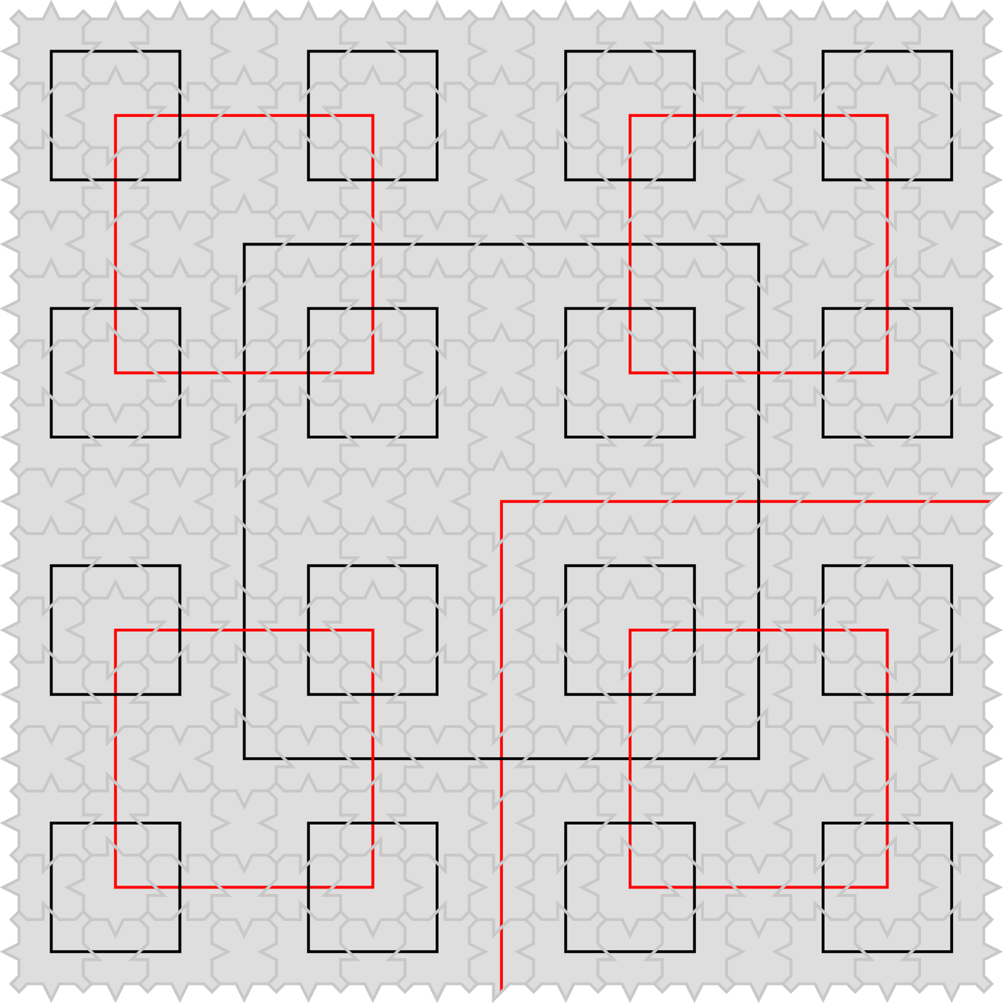
For the rest of this paper, a generic Robinson tiling will refer to a configuration without an infinite cut, such that any two tiles of $\mathds{Z}^{d}$ end up being in the same $n$ -macro-tile for big-enough values of $n$ . In such a generic configuration $\omega\in\Omega_{RB}$ , by induction, the $n$ -macro-tiles all have a central arm with the same colour. In particular, a generic configuration will only contain Red or Black bumpy-corners, never both.

Proposition 3.1.

Let $\Omega_{RB}$ be the Red-Black Robinson tiling. For any $\varepsilon>0$ , there is $\mu\in\mathcal{M}_{RB}^{\mathcal{B}}(\varepsilon)$ such that $d_{B}\left(\mu,\mathcal{M}_{RB}\right)\geq\frac{1}{8}$ . Thus, the SFT is unstable.

Proof.

The goal of this proof is to convert a generic tiling $\omega\in\Omega_{RB}$ into a random noisy tiling $\lambda_{\omega,b}$ on $\Omega_{\widetilde{RB}}$ , with $b$ a random variable on $\Omega_{\{0,1\}}$ . Using a generic Bernoulli noise $b$ in the input, we will obtain a noisy tiling for which its bumpy-corners are now half Red and half Black, which will yield the announced result since bumpy-corners have frequency $\frac{1}{4}$ in the Robinson tiling.

We will build this measure $\lambda$ iteratively, as a limit of a locally-defined (thus trivially measurable) transformations. At each step of the construction, the actual monochromatic structure of the Robinson tiling will be preserved, and only the colours will be mismatched, so we may still consider $n$ -macro-tiles in this structural sense, even though they are not actually locally admissible. We initialise $\lambda_{1}=\delta_{(\omega,b)}$ as a constant Dirac measure.

Let us now explain how we obtain $\lambda_{2}$ out of $\lambda_{1}$ . This transformation will be done independently on each of the $2$ -macro-tiles of $\omega$ . We distinguish two cases, both illustrated in Figure 4, where the black cells $c$ represent obscured tiles with a noise $b_{c}=1$ . A macro-tile is said to be flippable if both of its bi-coloured crosses, highlighted with green borders in the figure, are obscured tiles. In such a situation, we will flip its colours (Black lines become Red and conversely) with probability $\frac{1}{2}$ , independently of the rest, which still preserves the local rules inside the macro-tile. In the figure, the top-left macro-tile is flipped, the top-right macro-tile is flippable but not flipped, and the two bottom macro-tiles are not flippable.

Likewise, we go from $\lambda_{n-1}$ to $\lambda_{n}$ by flipping independently at random any flippable $n$ -macro-tile (except the two ends of the central arm that are “after” the bi-coloured crossed tiles, which must match the colour of the yet-unflipped corresponding $(n+1)$ -macro-tile). This process guarantees that, if we denote $\omega^{\prime}\sim\lambda_{n}$ the new colouring, then $\left(\omega^{\prime},b\right)\in\Omega_{\widetilde{RB}}$ almost-surely.

Notice how the highlighted cells that decide whether a given macro-tile is flippable are disjoint for each macro-tile. Hence, assuming that $b\sim\mathcal{B}(\varepsilon)^{\mathds{Z}^{2}}$ is a Bernoulli noise, each macro-tile at each scale is flippable with probability $\varepsilon^{2}$ , independently of the rest. With such a choice of noise $b$ , the weak-* limit $\lambda_{\omega,b}$ is well-defined.

Consider $G(\omega)\subset\mathds{Z}^{2}$ the set of cells containing a bumpy corner in $\omega$ . For a given cell $c\in G$ , we denote by $\text{flip}_{c,n}$ the random variable equal to $1$ when the $n$ -macro-tile containing $c$ is flippable. Hence the variables $\text{flip}_{c,n}\sim\mathcal{B}\left(\varepsilon^{2}\right)$ are iid. Conditionally to the event $\text{flip}_{c,n}=1$ , the colour of the cell $c$ is uniformly distributed in $\lambda_{n}$ after rank $n$ . Thence, by Borel-Cantelli lemma, the colour of $c$ is uniformly distributed in $\lambda_{\omega,b}$ .

Likewise, consider two distant cells $c,d\in G$ . As $d_{\infty}(c,d)\to\infty$ , the smallest rank $n_{0}(c,d)$ such that $c$ and $d$ belong to the same $n$ -macro-tile of $\omega$ goes to infinity. The families $\left(\text{flip}_{c,n}\right)_{n<n_{0}}$ and $\left(\text{flip}_{d,n}\right)_{n<n_{0}}$ are independent, and conditionally to the fact that both of these sequences contain at least a $1$ , the colours of cells $c$ and $d$ are independently uniform (in the measures $\lambda_{n}$ after rank $n_{0}$ , hence for $\lambda_{\omega,b}$ ).

Without loss of generality, assume $0\in G$ , so that $G=(2\mathds{Z})^{2}$ . Then the family $\left(\text{colour of the cell }2c\right)_{c\in\mathds{Z}^{2}}$ describes a $\sigma$ -invariant ergodic dynamical system, so that we may apply a pointwise ergodic theorem. This implies that the frequency of both Black and Red bumpy-corners is generically equal to $\frac{1}{2}$ in $\lambda_{\omega,b}$ . As $G$ has density $\frac{1}{4}$ in $\mathds{Z}^{2}$ , we conclude that for almost-any $\omega^{\prime}\sim\lambda_{\omega,b}$ and any generic $\omega_{0}\in\Omega_{RB}$ (with monochromatic bumpy-corners), we have the bound $d_{H}\left(\omega_{0},\omega\right)\geq\frac{1}{2}\times\frac{1}{4}=\frac{1}{8}$ assuming bumpy-corners overlap between the two configurations, and even a $\frac{1}{2}$ bound if they are misaligned.

We can conclude the proof by averaging $\lambda_{\omega,b}$ over $\omega\sim\mu_{0}\in\mathcal{M}_{RB}$ (chosen independently from $b$ ), which gives us at last a $\sigma$ -invariant measure $\mu\in\mathcal{M}_{RB}^{\mathcal{B}}(\varepsilon)$ that satisfies $d_{B}\left(\mu,\mathcal{M}_{RB}\right)\geq\frac{1}{8}$ . ∎

The result still holds with the very same proof if we replace the bi-coloured Robinson tiling by a bi-coloured variant of the structurally enhanced Robinson tiling from our previous paper [10].

However, as the proof relies heavily on flipping the colours of bumpy-corners, by keeping only one of the two colours specifically for this tile, we obtain a stable tiling again. This will be useful later on, when we want to encode Turing machines into Robinson (which requires this bi-coloured setting) in a stable way. In such situations, stability will follow from the result of the next section.

4. Generalising Aperiodic Stability

In order to prove the stable cases later on, we will state a direct generalisation of one of the main results in our previous article [10, Proposition 7.8]. This proposition was proven in the specific context of the enhanced Robinson tiling, but we will here reformulate the result in a general framework for quasi-periodic tilings with a well-behaved reconstruction function, so that it applies as a black box to the tilesets described in the next section. This section is here mostly for the sake of technical completeness, and can be skipped to focus on the core of the paper to which we go back right after.

Definition 4.1 (Almost Periodic SFT).

Let $\Omega_{\mathcal{F}}$ be a SFT on the alphabet $\mathcal{A}$ , and consider $p\in\mathds{N}^{*}$ and $\rho>0$ .

We say that $\Omega_{\mathcal{F}}$ is $\rho$ -almost $p$ -periodic if there is a $p$ -periodic “grid” $G\subset\mathds{Z}^{d}$ (invariant under translations in $(p\mathds{Z})^{d}$ ) of density at most $\rho$ , such that any configuration restricted to a translation of $G^{c}$ is made periodic. By this, we mean that for any $\omega\in\Omega_{\mathcal{F}}$ , there is a unique translation of $G$ (given by a non-necessarily unique $k\in\llbracket 0,p-1\rrbracket^{d}$ ) such that $\omega|_{G^{c}+k}$ is $p$ -periodic.

In this case, assuming $\square\notin\mathcal{A}$ , we can define $\omega^{\square}$ by overwriting $\omega|_{G+k}$ by the blank symbol $\square$ . Thence, $\Omega_{\mathcal{F}}^{\square}=\left\{\omega^{\square},\omega\in\Omega_{\mathcal{F}}\right\}$ is a finite $p$ -periodic SFT.

The non-uniqueness of $k$ comes from the fact that, for example, we may want to consider $G$ a $\frac{p}{2}$ -periodic grid instead, with some more redundancy in its structure.

Definition 4.2 ( $C$ -Reconstruction Function).

Consider $\Omega_{\mathcal{F}}$ a $\rho$ -almost $p$ -periodic SFT and $G$ the associated grid.

The SFT has the $C$ -reconstruction property if, for any locally admissible tiling $\omega$ of $B_{\left\lceil\frac{p}{2}\right\rceil+C}$ there is a unique translation of $G$ such that $\left[\omega|_{B_{\left\lceil\frac{p}{2}\right\rceil}\cap\left(G^{c}+k\right)}\right]^{\square}$ (obtained by filling $B_{\left\lceil\frac{p}{2}\right\rceil}\cap\left(G+k\right)$ with $\square$ symbols) is globally admissible in $\Omega_{\mathcal{F}}^{\square}$ (thence $\omega|_{B_{\left\lceil\frac{p}{2}\right\rceil}\cap\left(G^{c}+k\right)}$ is globally admissible in $\Omega_{\mathcal{F}}$ ). What’s more, the translation of $G$ depends only on what happens in any $p$ -square included in the central window $B_{\left\lceil\frac{p}{2}\right\rceil}$ (which is either a $(p+1)$ or $(p+2)$ -square depending on the parity).

As $\Omega_{\mathcal{F}}^{\square}$ is $p$ -periodic, there is a unique choice $\omega^{\square}\in\Omega_{\mathcal{F}}^{\square}$ of configuration that will match the pattern $\left[\omega|_{B_{\left\lceil\frac{p}{2}\right\rceil}\cap\left(G^{c}+k\right)}\right]^{\square}$ .

Proposition 4.1 (Besicovitch Bound).

Consider a $\rho$ -almost $p$ -periodic SFT with $C$ -reconstruction. Then, for any $\varepsilon>0$ and $\mu\in\mathcal{M}_{\mathcal{F}}^{\mathcal{B}}(\varepsilon)$ , we have the bound $d_{B}\left(\mu,\mathcal{M}_{\mathcal{F}}\right)\leq 48\left(2\left(C+\left\lceil\frac{p}{2}\right\rceil\right)+1\right)^{d}\varepsilon+\rho$ .

Proof.

The proof is really similar to the source result [10, Proposition 7.8], so we will just give the general idea.

Consider $\lambda\in\widetilde{\mathcal{M}_{\mathcal{F}}^{\mathcal{B}}}(\varepsilon)$ and $(\omega,b)\in\Omega_{\widetilde{\mathcal{F}}}$ a $\lambda$ -generic noisy configuration. A percolation argument [10, Proposition 5.6] tells us that, almost-surely, we can forget about the $\left(C+\left\lceil\frac{p}{2}\right\rceil\right)$ -neighbourhood of obscured cells (cells $c\in\mathds{Z}^{d}$ with $b_{c}=1$ ) and still have a unique connected component of clear cells ( $b_{c}=0$ ) with density of at least $48\left(2\left(C+\left\lceil\frac{p}{2}\right\rceil\right)+1\right)^{d}\varepsilon$ .

Each clear cell $c$ of this connected component is the center of a clear window $I_{c}$ of diameter $2\left\lceil\frac{p}{2}\right\rceil+1$ , the $C$ -neighbourhood of which is clear and locally admissible, so by the $C$ -reconstruction property, there is a unique translation of $G$ and a unique periodic configuration $\omega_{c}^{\square}\in\Omega_{\mathcal{F}}^{\square}$ that matches $\omega$ on $I_{c}\cap(G+k)^{c}$ (for the right translation). We can do likewise for any other cell.

Now, two neighbouring cells $c,c^{\prime}\in\mathds{Z}^{d}$ share a common $p$ -square window which fixes the same choice of translation for $G$ . Hence, $\omega_{c}^{\square}$ and $\omega_{c^{\prime}}^{\square}$ overlap on this $p$ -square, and $\Omega_{\mathcal{F}}^{\square}$ is $p$ -periodic, so they are equal. Thus, all the cells of the infinite connected component $I(b)$ must agree on the same $\omega^{\square}$ . The map $\varphi:(\omega,b)\mapsto\omega^{\square}$ is measurable (for $\varepsilon$ small-enough, so that $I$ has density greater than $\frac{1}{2}$ ).

In particular, $\omega$ and $\omega^{\square}$ can only differ outside of $I(b)$ , or on the translation of $G$ , so $d_{H}\left(\omega,\omega^{\square}\right)\leq\text{density}(I)+\text{density}(G)\leq 48\left(2\left(C+\left\lceil\frac{p}{2}\right\rceil\right)+1\right)^{d}\varepsilon+\rho$ , and the same bound holds for $d_{B}\left(\pi_{1}^{*}(\lambda),\varphi^{*}(\lambda)\right)$ . At last, we can fill-in the $\square$ symbols of $G$ in an appropriate random way, in order to send $\varphi^{*}(\lambda)$ into $\mathcal{M}_{\mathcal{F}}$ , without changing the bound on $d_{B}$ . ∎

In particular, this proposition gives us a linear $O(\varepsilon)$ bound for the stability of any actually periodic tiling (which will be $0$ -almost periodic, with $G=\emptyset$ and $C$ -reconstruction for some $C$ ).

However, it doesn’t apply to the Red-Black tiling from the previous section, for which we can juxtapose side by side a Red and a Black $n$ -macro-tile at any scale in a locally admissible way, which breaks the desired quasi-periodicity.

Corollary 4.2 (Stability).

Assume there is a sequence of triplets $\left(p_{n},\rho_{n},C_{n}\right)$ for which Proposition 4.1 applies to $\Omega_{\mathcal{F}}$ . Then, as soon as $\rho_{n}\to 0$ , we conclude that $\Omega_{\mathcal{F}}$ is a stable SFT.

Lemma 4.3 (Meta Multi-Scale-to-Polynomial Bound).

Consider $D_{k}=\varepsilon\alpha^{k}+\beta^{k}$ with $k\in\mathds{Z}$ and $0<\beta<1<\alpha$ . Denote $\theta=\log_{\alpha}\left(\frac{1}{\beta}\right)=\frac{-\ln(\beta)}{\ln(\alpha)}>0$ . Then, for any choice $K\in\mathds{Z}$ , the following bound holds as long as $\varepsilon\leq\frac{\theta}{\alpha^{K(1+\theta)}}$ :

\min_{k\geq K}D_{k}\leq\max\left(\sqrt{\alpha},\sqrt{\frac{1}{\beta}}\right)\times\left(\theta^{\frac{1}{1+\theta}}+(1/\theta)^{\frac{1}{1+1/\theta}}\right)\times\varepsilon^{\frac{\theta}{1+\theta}}.

Proof.

We will later on find the optimal bound on the right assuming $k\in\mathds{R}$ . Then, by replacing $k$ with the nearest integer we will either increase the power of $\alpha$ by $\frac{1}{2}$ or decrease the one of $\beta$ by $\frac{1}{2}$ . Note that this bound works best under the assumption that $\alpha\approx\frac{1}{\beta}$ . If one is much bigger than the other, we may simply decide on which side we always round $k$ , with an added factor $\alpha$ or $\frac{1}{\beta}$ instead.

Now, consider the parameter $x:=\alpha^{k}\in\mathds{R}^{+*}$ . Thus, $k=\log_{\alpha}(x)$ so:

\beta^{k}=\exp\left(\frac{\ln(x)}{\ln(\alpha)}\times\ln(\beta)\right)=\exp\left(-\theta\ln(x)\right)=x^{-\theta}.

With this rewriting, $D(x):=\varepsilon x+x^{-\theta}$ is much easier to minimise. Indeed, $D$ can be seen as a positive convex function that goes to $+\infty$ on $0^{+}$ and $+\infty$ , hence is minimised when $D^{\prime}(x):=\varepsilon-\theta x^{-\theta-1}=0$ , thus at $x=\left(\frac{\theta}{\varepsilon}\right)^{\frac{1}{\theta+1}}$ . Using this value of $x$ in $D$ directly gives us the rest of the expected bound.

Now, for the domain of validity, for us to be ably to round $k$ properly, we simply require $k=\log_{\alpha}(x)\geq K$ , which translates as $\varepsilon\leq\frac{\theta}{\alpha^{K(1+\theta)}}$ . When the bound doesn’t hold, when $K$ is greater that the optimal value, the optimal choice is simply $D_{K}$ . ∎

Corollary 4.4 (Polynomial Stability).

Assume there is a sequence of triplets $\left(p_{n},\rho_{n},C_{n}\right)$ for which Proposition 4.1 applies to $\Omega_{\mathcal{F}}$ . If $C_{n}+p_{n}=O\left(\alpha^{\frac{n}{d}}\right)$ and $\rho_{n}=O\left(\beta^{n}\right)$ , then using the previous lemma gives us a polynomial bound $O\left(\varepsilon^{\frac{\theta}{1+\theta}}\right)$ on the speed of convergence, with $\theta=\frac{-\ln(\beta)}{\ln(\alpha)}$ .

Remark 4.1.

To illustrate how this framework applies, let us use it to obtain the polynomial stability for the enhanced Robinson tiling.

Unlike the usual Robinson tiling, the enhanced variant enforces alignment of neighbouring macro-tiles in a local way. At the scale of $N$ -macro-tiles, if we forget about the grid around these tiles, of density $\rho_{n}=1-\frac{\left(2^{n}-1\right)^{2}}{4^{n}}=O\left(\frac{1}{2^{n}}\right)$ , we obtain a $p_{n}$ -periodic tiling with $p_{n}=2\times 2^{n}$ . What’s more, we can prove the tiling has $C_{n}$ -reconstruction [10, Proposition 7.7], with a radius $C_{n}=2^{n}-1$ . As we have $C_{n}+p_{n}=O\left(2^{n}\right)=O\left(4^{\frac{n}{2}}\right)$ , we can apply the previous corollary with parameters $(\alpha,\beta)=\left(4,\frac{1}{2}\right)$ , so $\theta=\frac{1}{2}$ and $\frac{\theta}{1+\theta}=\frac{1}{3}$ . Hence, we fall back on the $O\left(\sqrt[3]{\varepsilon}\right)$ bound of the previous article [10, Theorem 7.9] (with a comparable multiplicative constant) which is to be expected as we basically generalised the scheme of the proof used in that paper.

More generally, in a hierarchical tiling, at the scale of “macro-tiles” of diameter $x$ , the typical reconstruction radius we may hope for is of order $x$ at least (i.e. the size of a macro-tile), and likewise for the quasi-periodicity. Conversely, among the $x^{d}$ cells in a macro-tile, we may have to ignore at least a one-dimensional “wire” that crosses the whole macro-tile, hence hence $\rho$ of order $\frac{1}{x^{d-1}}$ at least. Following the same general computations as in the previous lemma, we conclude that in $d$ dimensions, the best speed of convergence we may obtain is $O\left(\varepsilon^{\frac{d-1}{2d-1}}\right)$ . With $d=2$ , we have $\frac{d-1}{2d-1}=\frac{1}{3}$ , the order of convergence obtained for the enhanced Robinson tiling. The question of whether we can obtain a faster bound for the convergence speed of aperiodic tilings, whether by improving upon the minimal values of $(C,p,\rho)$ conjectured here (and in particular on the $C$ -reconstruction), or by using another method altogether, is still open.

5. Undecidability of the Stability

In the previous sections, we showed how a simple bi-coloured tiling can be unstable, and how a class of well-behaved quasi-periodic SFTs can be stable. We will now make full use of these ideas in order to equate the notion of stability with some undecidable problems in the arithmetical hierarchy through the emergence of said unstable structure.

Matter-of-factly, proving $\Pi_{2}$ -hardness would directly imply the weaker bounds we introduce first. However, the $\Pi_{2}$ -hard construction relies on the $\Sigma_{1}$ -hard one, and we believe the $\Pi_{1}$ -hard one uses a complementary and more intuitive idea that will help get the point across.

5.1. $\Pi_{1}$ -hard construction

First, we will make use of the halting problem $P_{halt}$ . What we want to do here is to encode computations into the Robinson tiling in a stable way, and make an unstable phase emerge iff the machine terminates. This will equate the $\Sigma_{1}$ -complete halting problem with instability among a class of SFTs, hence $\Pi_{1}$ -hardness of $P_{stab}$ in general.

In the previous Red-Black example of Section 3, the main ingredient allowing instability was the existence of two kinds of $n$ -macro-tiles at any scale (widely different for the finite Hamming distance) instead of just one (four similar tiles, up to the orientation of their low-density central cross) in the monochromatic case. The two kinds of macro-tiles cannot coexist in the same generic Robinson configuration, but we can replace one with the other for a small price in the presence of noise.

5.1.1. Description of the Tileset

Let us first describe the tileset used in this section. We won’t explain in details how Turing machines can be implemented inside the Robinson tiling, but the interested reader may look at the original article by Robinson [25] or lecture notes by Jeandel and Vanier [20] for a formal study of this simulation result.

We will use a variant of this construction more suited to our needs, with two layers, defined on the alphabet $\mathcal{A}\subset\mathcal{A}_{R}\times\mathcal{A}_{M}$ , where $\mathcal{A}_{R}$ stands for the common Robinson layer, and $\mathcal{A}_{M}$ for the layer specific to a given Turing machine $M$ . Consequently, we will denote $\Omega_{P_{1}(M)}$ the corresponding SFT.

Let’s first describe the common layer $\mathcal{A}_{R}$ . As we can see in Figure 5, the tileset uses four main colours, as well as grey dotted and dashed lines. These grey lines must match with one of the same type (either dotted or dashed on both sides of an edge), and serve to enforce alignment of the Robinson macro-tiles locally, to guarantee stability of the structure itself, just like for the enhanced Robinon tiling [10, Proposition 7.7]. Notice how bumpy-corners must be Black, after which we alternate between Black and Red. At some point, to-be-decided by the layer $\mathcal{A}_{M}$ , we may transition from the Red-Black (stable) regime to the Blue-Green (unstable) regime using one of the two transition tiles on the bottom-right of Figure 5. The whole set $\mathcal{A}_{R}$ is given by all the rotations of the first three columns (but no symmetry, so that we may preserve the chirality of macro-tiles, so that each arm of the central cross may indicate the overall orientation of the macro-tile) and rotations and symmetries of the rest, which brings us to a total of $\left|\mathcal{A}_{R}\right|=172$ tiles.

Now, without detailing the intricacies of $\mathcal{A}_{M}$ and how it is coupled with $\mathcal{A}_{R}$ in $\mathcal{A}$ , let us give the general idea and specificities of our construction. Here, each Red square (of length $4^{n}+1$ , in the center of a $(2n+1)$ -macro-tile) will contain a limited space-time diagram of the Turing machine $M$ with a semi-infinite ribbon, while avoiding smaller red squares which contain their own space-time diagram. This is illustrated in Figure 6, where the black crossed cells represent the patches of space-time diagram, and the grey cells are communication channels that synchronise the otherwise disconnected patches of the diagram. The $n$ -th scale of simulation, occurring in a $(2n+1)$ -macro-tile, thus has a space-time horizon of $2^{n}+1$ tiles, initiated on the empty input on the bottom row.

The main difference with the canonical construction is how it behaves when $M$ stops. In Robinson’s article, the tiling doesn’t allow for $M$ to stop, in order to prove that the tileability problem is undecidable. Here, when $M$ halts in the $n$ -th scale of simulation, it idles until the border of the square can “notice” the halting, and decide freely whether it will force a transition from Black to Blue or Green on its border. After which, at higher scales, no more computations occur. Still, whether or not this transition occurs, we have arbitrarily big macro-tiles, and thus $\Omega_{P_{1}(M)}\neq\emptyset$ . Note that a description of $M$ can be algorithmically converted into the set of forbidden patterns $P_{1}(M)$ (and its corresponding alphabet) in finite time.

Theorem 5.1 ( $P_{stab}$ is $\Pi_{1}$ -hard).

Consider a Turing machine $M$ . Then the SFT defined by $P_{1}(M)$ is stable ( $P_{1}(M)\in P_{stab}$ ) iff $M$ does not halt on the empty input ( $M\notin P_{halt}$ ). As $P_{halt}$ is $\Sigma_{1}$ -complete, we deduce that $P_{stab}$ is $\Pi_{1}$ -hard.

The following subsubsections will each focus on one of the implications, which put together directly give the previous result.

5.1.2. The Stable Case

For the stable case, assume that $M\notin P_{halt}$ . Because of this, at any scale of admissible macro-tiles, the previously described transition from the Red-Black to the Blue-Green regime cannot occur, and the two last lines of tiles in Figure 5 may as well not exist in $\mathcal{A}_{R}$ . Our goal is to prove that the framework of Section 4 applies here.

Notice how we can project the alphabet $\mathcal{A}$ onto its first coordinate $\mathcal{A}_{R}$ and then erase the information on which of the four colours is used for the lines atop of a tile. This way, we fall back on the enhanced Robinson tiling studied in our previous paper. In particular, the following structural result applies:

Proposition 5.2 ([10, Proposition 7.7]).

Consider the enhanced Robinson SFT. Let us denote $B_{k}=\llbracket-k,k\rrbracket^{2}$ . For any scale of macro-tiles $n\geq 2$ , the constant $R_{n}=2^{n}-1$ is such that, for any $k\geq 0$ and any clear locally admissible pattern $\omega$ on $B_{k+R_{n}}$ , its restriction $\omega|_{B_{k}}$ is made of well-aligned and orientated $n$ -macro-tiles, plus the grid around them which we do not control.

Thence, at the $n$ -th scale of simulation (i.e. in $(2n+1)$ -macro-tiles), the tiling $\Omega_{P_{1}(M)}$ is $\frac{1}{4^{n}}$ -almost $p_{n}$ -periodic (with $p_{n}=4^{n+1}$ ) with $C_{n}$ -reconstruction ( $C_{n}=R_{2n+1}$ ) if we specifically look at the layer $\mathcal{A}_{R}$ . However, we need to tread a bit more carefully to obtain the desired periodic behaviour on the other coordinate of the alphabet $\mathcal{A}$ , and we will actually specifically extend the grid around $(2n+1)$ -macro-tiles into a larger set $G_{n}$ to do so.

Lemma 5.3.

Using the constant choices from the previous paragraph, the SFT $\Omega_{P_{1}(M)}$ is $\rho_{n}$ -almost $p_{n}$ -periodic with $C_{n}$ -reconstruction, with $G_{n}$ the area outside of Red squares up to the $n$ -th scale and $\rho_{n}$ its density.

Proof.

Because $\Omega_{P_{1}(M)}$ enforces alignment in a local way, for any tiling $\omega$ we obtain the same set $G_{n}$ (up to translation) by looking at all the tiles outside of Red squares up to the $n$ -th scale of simulations. This $G_{n}$ is $p_{n}$ -periodic, and in particular includes the grid surrounding $(2n+1)$ -macro-tiles so that we have $\rho_{n}$ -quasi $p_{n}$ -periodicity with $C_{n}$ -reconstruction on the layer $\mathcal{A}_{R}$ .

Regarding alignment, notice that $G_{n}$ has the same periodicity as the grid around $(2n+1)$ -macro-tiles, whose alignment is fixed by the $C_{n}$ -reconstruction on the layer $\mathcal{A}_{R}$ , hence its alignment is fixed in the same way.

Remark that, on the layer $\mathcal{A}_{M}$ , because the Turing machine is deterministic, everything that happens on the inside of a given admissible Red square is fixed, insulated from outside interference. Hence, on this layer (and using of course the alignment of $G_{n}$ given by the layer $\mathcal{A}_{R}$ ) we obtain a $\frac{p_{n}}{2}$ -periodic behaviour outside of $G_{n}$ , as it does not depend on the orientation of the $(2n+1)$ -macro-tiles. ∎

In order to conclude, we need to compute $\rho_{n}$ the density of $G_{n}$ .

Lemma 5.4.

In a $(2n+1)$ -macro-tile, we have $O\left(12^{n}\right)$ tiles outside of the Red squares.

Proof.

The general idea of the proof is that Red squares form a kind of Sierpiński carpet inside macro-tiles.

Denote $r_{n}$ the number of tiles inside the Red squares in a $(2n+1)$ -macro-tile. As we can see on Figure 3, in the process of forming a $(2n+3)$ -macro-tile, we will create a big central square around four $(2n+1)$ -macro-tiles, surrounded by twelve $(2n+1)$ -macro-tiles. As we already know the size of this big square, we obtain the following recurrence:

r_{n+1}=12r_{n}+\left(4^{n+1}+1\right)^{2}\geq 12r_{n}+16^{n+1}.

As $r_{1}=25\geq 16$ , we obtain by induction $r_{n}\geq 4^{n+1}\left(4^{n}-3^{n}\right)$ . At the same time, a $(2n+1)$ -macro-tile has $\left(2^{2n+1}-1\right)^{2}\leq 4^{2n+1}$ tiles in total, so at most $4^{n+1}3^{n}=4\times 12^{n}$ tiles outside the Red squares. ∎

Hence, as $(2n+1)$ -macro-tiles use $\Theta\left(16^{n}\right)$ tiles in total, we conclude that $G_{n}$ has density $\rho_{n}=O\left(\left(\frac{3}{4}\right)^{n}\right)$ .

Proposition 5.5.

Consider $M\notin P_{halt}$ . Then $\Omega_{P_{1}(M)}$ is polynomially stable, with convergence speed $O\left(\varepsilon^{r}\right)$ at rate $r=\frac{2-\log_{2}(3)}{6-\log_{2}(3)}\approx 0.094$ .

Proof.

We apply Corollary 4.4, with constants $\alpha=4$ and $\beta=\frac{3}{4}$ , so $r=\frac{\theta}{1+\theta}$ gives the announced rate. ∎

5.1.3. The Unstable Case

Proposition 5.6.

Assume $M\in P_{halt}$ . Then for any $\varepsilon>0$ we have a measure $\mu\in\mathcal{M}_{P_{1}(M)}^{\mathcal{B}}(\varepsilon)$ such that $d_{B}\left(\mu,\mathcal{M}_{P_{1}(M)}\right)\geq\frac{1}{4^{n+1}}$ , where $n$ denotes the last scale of simulation, at which $M$ halts.

Proof.

Consider $N=2(n+1)$ the first scale at which $N$ -macro-tiles have a big Blue or Green square in the middle. Assuming two aligned $N$ -macro-tiles don’t use the same colour for the square (of diameter $d=2^{N-1}+1$ tiles), then we obtain at least $p=4\times(d-1)=2^{N+1}$ differences.

By following the very same colour-flipping process as in Proposition 3.1, but on the Blue-Green bit starting at the scale of $N$ -macro-tiles, we obtain a generic colour-flipped configuration $\omega$ (with monochromatic Blue or Green squares in the $N$ -macro-tiles).

Thus, for any generic $\omega\in\Omega_{P_{1}(M)}$ that aligns with $\omega^{\prime}$ up to the scale of $N$ -macro-tiles, we obtain a lower bound $d_{H}\left(\omega,\omega^{\prime}\right)\geq\frac{1}{2}\times\frac{p}{4^{N}}=\frac{1}{2^{N}}=\frac{1}{4^{n+1}}$ , with the factor $\frac{1}{2}$ coming from the frequency of Blue and Green big squares in $\omega^{\prime}$ , whereas all such squares of $\omega$ must be of the same colour.

Now, assume that $N$ -macro-tiles in $\omega$ and $\omega^{\prime}$ don’t align well. By choosing the best pairing of $N$ -macro-tiles between $\omega$ and $\omega^{\prime}$ , we still have a rectangle with both sides of length at least $2^{N-1}-1$ (the size of a $(N-1)$ -macro-tile) where the $N$ -macro-tiles of both tilings overlap. In this area, both macro-tiles have a Blue or Green corner of their big square, made of at least $2\times\left(2^{N-1}+1\right)$ tiles. As these two corners intersect in at most $2$ tiles, and the rest of the area is guaranteed to use only Black or Red communication channels, we have at least $2^{N}$ differences between $\omega$ and $\omega^{\prime}$ in this window. As this process repeats $2^{N}$ periodically in both directions, without even having to take the colour-flipping into account, we still obtain $d_{H}\left(\omega,\omega^{\prime}\right)\geq\frac{1}{2^{N}}=\frac{1}{4^{n+1}}$ . ∎

Remark 5.1.

More generally, as long as we can guarantee one difference between the two kinds of macro-tiles which we colour-flip, we obtain a lower bound on $d_{B}$ of order $\frac{1}{\text{tile area}}$ . We will directly invoke this “obvious” lower bound for further unstable cases.

Still, the order of magnitude $\frac{1}{\text{tile diameter}}$ obtained in the previous proposition is the best one can reasonably hope for in general, as a signal that transits through a macro-tile will typically only cross a number of tiles proportional to the diameter, normalised by the tile area.

5.2. $\Sigma_{1}$ -hard Construction

We can “flip around” the previous construction, by adding an unstable information atop of the structure simulating the Turing machine, in such a way that the information gets frozen and becomes stable if the machine halts. We will first describe the construction of $S_{1}(M)$ out of a machine $M$ , and then state the corresponding indecidability result.

In the previous tileset $P_{1}(M)$ , the Robinson layer $\mathcal{A}_{R}$ used one communication channel with four different colours. Here, for $S_{1}(M)$ , we use two communication channels in the lines of the Robinson structure, each one having two possible values. First, the Red-Black channel must be initialised as Black in bumpy corners, and then alternate, in order to have the right structure to simulate the machine $M$ . Second, the Blue-Green channel can be freely initialised. However, if $M$ halts at a given scale of simulation, then the border of the Red square must be Blue on the other channel, which we call a freeze. Note that here, we can keep simulating $M$ at higher scales after it halts for the first time, as subsequent freezes will just occur at scales of macro-tiles where the Blue-Green channel would be frozen into Blue anyway.

Proposition 5.7.

We have $S_{1}(M)\in P_{stab}$ iff $M\in P_{halt}$ . Thus, $P_{stab}$ is $\Sigma_{1}$ -hard.

Proof.

First, assume that $M\notin P_{halt}$ . Then we can freely do a colour-flipping process starting from any $\mu\in\mathcal{M}_{S_{1}(M)}$ , just like in Proposition 3.1. We can start flipping the Blue-Green channel at the scale of bumpy corners, hence instability with a $\frac{1}{8}$ lower bound on $d_{B}$ .

Now, assume $M\in P_{halt}$ . Then, in any tiling $\omega\in\Omega_{S_{1}(M)}$ , the Blue-Green channel is retroactively frozen all the way down to the Green bumpy-corners. By using the same grid $G_{n}$ as in Lemma 5.3, we can likewise ignore everything that happens outside of Red squares, and control everything inside, hence a $\rho_{n}$ -almost $p_{n}$ -periodic tiling with $p_{n}=O\left(4^{n}\right)$ and $\rho_{n}=O\left(\left(\frac{3}{4}\right)^{n}\right)$ .

Finally, denote $n_{halt}$ the first scale of simulation at which $M$ halts in $S_{1}(M)$ . If we try to reconstruct things locally at steps lower than $n_{halt}$ , then we will reach a family of well-aligned and well-oriented $(2n+1)$ -macro-tiles, but without any freezing happening in the tiles, hence this Blue-Green channel that may not behave in a globally admissible way, all the way down to the high-density set of bumpy-corners. Still, as long as $n\geq n_{halt}$ , the freezing prevents this from happening, and using the same $C_{n}=O\left(4^{n}\right)$ as in Lemma 5.3, we conclude that this scale of the tiling has indeed $C_{n}$ -reconstruction.

Still, starting at high-enough scales, for low-enough values of $\varepsilon$ , the proof of Proposition 5.5 applies verbatim, so we have stability with a polynomial $O\left(\varepsilon^{r}\right)$ convergence rate. ∎

5.3. $\Pi_{2}$ -hard Construction

In the construction for $S_{1}(M)$ , we obtained stability iff there exists a time step such that $M$ halts on the empty input. Consequently, if we manage to twist the construction to include any possible input, then we may equate stability with the $\Pi_{2}$ -complete totality problem $P_{total}$ .

There are several ways to proceed, but we choose here to use the method of Toeplitz encoding of the input, because it is quite versatile, and may more generally be able to convert a (structurally close to) uniquely ergodic SFT encoding a $\Sigma_{k}$ -hard problem into a (definitely not uniquely ergodic anymore) SFT encoding a $\Pi_{k+1}$ -hard problem.

5.3.1. Toeplitz Input

The Toeplitz encoding of an infinite sequence $u\in\Gamma^{\mathds{N}^{*}}$ on an alphabet $\Gamma$ consists of inductively filling with $u_{n}$ half of the holes still free after the previous iterations, which gives a sequence $u_{1}*u_{1}*u_{1}*u_{1}*\dots$ , then $u_{1}u_{2}u_{1}*u_{1}u_{2}u_{1}*\dots$ , and so on. Toeplitz sequences have been studied as dynamical systems for a long while [17], and have since been encoded in higher-dimensional SFTs [6].

The idea of the method is to sequentially write the wanted input $u$ into the consecutive scales hierarchical structure, which will appear as a Toeplitz encoding $u_{1}u_{2}u_{1}\dots$ from the point of view of the simulated Turing machine, and then adapt the machine to decode it back into its original form $u$ at first. This method was already used by Barbieri and Sablik [4] in particular.

More precisely, we build the tileset $P_{2}(M)$ as follows. For the Robinson structure, we use the same parallel Red-Black and Blue-Green bits as for $S_{1}(M)$ . We add another channel that can take values in $\Sigma\sqcup\{\#,\$^{\Sigma},\$^{\#}\}$ where $\Sigma$ is the input alphabet of the machine $M$ , $\#$ the blank tape symbol, and the $\$^{*}$ symbols two supplementary letters. On Black channels, we can freely use any symbol $\$^{*}$ following a letter from $\Sigma$ on the previous Red scale, but we must use $\$^{\#}$ following $\#$ . On Red channels, we must use a letter from $\Sigma$ following a $\$^{\Sigma}$ symbol on the previous Black scale, and use $\#$ following $\$^{\#}$ . If we look only at the Red channels, this gives an infinite word $u\in\Sigma^{*}\#^{\mathds{N}}\sqcup\Sigma^{\mathds{N}}$ . When $u\in\Sigma^{*}\#^{\mathds{N}}$ , we will identify it with its prefix in $\Sigma^{*}$ , followed by $\#^{\mathds{N}}$ .

Quite importantly, the choice of a letter is not only communicated along the regular Red-Black channels in two directions from the center of a macro-tile arm, but also along the alignment channels of the enhanced Robinson self-aligning structure, the dotted and dashed lines in the other two directions. Thus, any two (well-aligned) neighbouring $N$ -macro-tiles must encode the same sequence.

On the simulation layer, the Turing machine is able to read which symbol is written down in the column on the right of its current position. Hence, from the point of view of the Turing machine simulated in a Red square, this represents a read-only second tape. In order to adequately use $u$ as an input, we first need to explain what the machine sees.

Lemma 5.8 (Toeplitz Encoding of the Input).

Let $u\in\Sigma^{*}\#^{\mathds{N}}\sqcup\Sigma^{\mathds{N}}$ . Define $w_{n}=w_{n-1}u_{n}w_{n-1}$ by induction, initialised with the empty word $w_{0}$ . The word $w_{n}$ is a prefix of the Toeplitz encoding of the whole sequence $u$ .

At the $n$ -th scale of simulation, from the point of view of the Turing machine, the read-only tape reads as $w_{n-1}\$^{*}\$^{*}w_{n-1}u_{n}$ .

Proof.

The last letter of the read-only ribbon obviously correspond to the right border of the $n$ -th Red square, hence reads as $u_{n}$ . The central $\$^{*}$ symbols come from the fact, as highlighted by the blue columns in Figure 7, they correspond to the $(n+1)$ -th scale for Black squares followed by the first scale of bumpy corners.

The rest of the word, that reads as $w_{n-1}$ on both ends of this central line, can be explained by the inductive construction of macro-tiles. Indeed, each quarter of the $n$ -th Red square is actually a whole $(2n-1)$ -macro-tile with a central Red square, and the Red squares are themselves stacked in a Toeplitz way within the macro-tile, with a gap in-between each that allows to read the letter on them. ∎

5.3.2. From Decoding the Input to Computations

Let us explain what Turing machine is encoded into $P_{2}(M)$ , and how it affects the Blue-Green channel.

First, the machine will have to decode the Toeplitz input, while keeping the Blue-Green channel stable (by using a third non-alternating colour). More precisely, the machine will step by step read the letters at positions $2^{k}$ on the read-only tape and write them one after another at the beginning of its working tape. This process will decode the Toeplitz encoding $w_{n}$ back into the sequence $u_{1}\dots u_{n}$ . Using a unary counter, which we multiply by two after reading each letter, reaching the $k$ -th letter will require about $\Theta\left(4^{k}\right)$ steps of computation.

Now, this process can halt in two ways. First, we read a $\$^{*}$ symbol, meaning that we reached halfway through the read-only ribbon. In this case, the machine simply idles for the rest of its finite runtime, without unfreezing the Blue-Green bit when it reaches the top border of the Red square. This won’t happen at big-enough scales of simulation, considering it would take about $\Theta\left(4^{n}\right)$ steps but the $n$ -th machine only has a finite horizon of $2^{n}$ steps, but it can occur at the initial scales of simulation and in particular at the very first one where the first symbol is $\$^{*}$ . Second, we read a $\#$ symbol before reaching the central $\$^{*}$ , in which case the decoding of the word $u\in\Sigma^{*}$ is complete. Without waiting, the machine starts then simulating $M$ on $u$ (this will occur roughly at the $2|u|$ -th scale of simulation). This will signal the Red square to ignite the unstable Blue-Green bit (if it was not already done at a lower scale), as was the case for $P_{1}(M)$ in Subsection 5.1. Then, if $M$ halts on $u$ , this will signal the Red square to freeze the Blue-Green bit, as was the case for $S_{1}(M)$ in Subsection 5.2.

5.3.3. Undecidability of the Stability

Lemma 5.9.

Assume $M\notin P_{total}$ does not halt on the input $u\in\Sigma^{*}$ . Consider $\mu_{u}\in\mathcal{M}_{\mathcal{F}}$ an invariant measure with $u\#^{\mathds{N}}$ written in the Red scales of any generic configuration. Then, by colour-flipping the Blue-Green channel after the inital decoding scales, we obtain the measure $\mu_{u}^{\varepsilon}\in\mathcal{M}_{\mathcal{F}}^{\mathcal{B}}(\varepsilon)$ , such that $\inf\limits_{\varepsilon>0}d_{B}\left(\mu_{u}^{\varepsilon},\mathcal{M}_{\mathcal{F}}\right)>0$ .

Proof.

As in Proposition 5.6, if we compare two macro-tiles with a Blue or Green square, corresponding to the same input $u\#^{\mathds{N}}$ , we can obtain a lower bound on their density of mismatching purely through the Blue-Green square.

Likewise, if we compare such a macro-tile with a macro-tile corresponding to another input, then they must differ in one of the first $|u|+1$ letters in a Red channel. In this case, we can also obtain a lower bound independent of $\varepsilon$ , even if they are perfectly aligned, using this mismatching letter in the input. ∎

Proposition 5.10.

Denote $\varphi(n)$ the first scale of simulation at which, for any input $u\in\Sigma^{\leq n}$ , both decoding and computation are over. Assume $M\in P_{total}$ , so that $\varphi(n)<\infty$ . Then, using the notations of Lemma 5.3, the SFT $\Omega_{P_{2}(M)}$ is $\rho_{n}$ -almost $p_{n}$ -periodic with $C_{\varphi(n)}$ -reconstruction.

Proof.

If we follow the same scheme of proof as in the lemma, then we almost obtain a $\rho_{n}$ -almost $p_{n}$ -periodic SFT with $C_{n}$ -reconstruction up to one detail.

Here, the Red-Black channel and all the computations in Red squares behave deterministically, so they are fixed for a given input (which synchronises between neighbouring tiles), but the Blue-Green channel is not. However, if we exploit the $C_{\varphi(n)}$ -reconstruction of the Robinson structure, then either:

•

a given Red square isn’t done decoding its input, so the Blue-Green bit is still frozen, uniquely determined,
•

a given Red square has decoded its input $u$ , at a scale of simulation lower than $n$ , which implies $|u|<n$ , but the Red square actually fits into a bigger $(2\varphi(n)+1)$ -macro-tile, which will terminate its simulation of $M$ on $u$ , thus freeze the Blue-Green bit of this Red square.

In both cases, we indeed guaranteed that the area inside Red squares is globally admissible, hence the $n$ -th scale of simulation admits $C_{\varphi(n)}$ -reconstruction. ∎

In particular, $\rho_{n}\to 0$ so $\Omega_{P_{2}(M)}$ is stable according to Corollary 4.2. However, because $\varphi$ can be roughly as big as any computable function, we can’t possibly exhibit a good bound to apply Corollary 4.4, and will not obtain polynomial stability this time. The next theorem directly follows:

Theorem 5.11.

Consider a Turing machine $M$ . We have $M\in P_{total}$ iff $P_{2}(M)\in P_{stab}$ . As $P_{total}$ is $\Pi_{2}$ -complete, we deduce $P_{stab}$ is $\Pi_{2}$ -hard.

Note how this process doesn’t adapt to translate the $\Pi_{1}$ -hard construction into a $\Sigma_{2}$ -hard one. In order to do this, we would need an added universal quantifier, which cannot work if we encode only one input at a time in a ground configuration. Hence, in this case we would need to enumerate the inputs inside the tiling in any case.

Remark 5.2 (Alternate Construction for $\Pi_{2}$ -Hardness).

Let us conclude this section by briefly describing another construction relating $P_{stab}$ to $P_{total}$ , this time without having to encode any input.

The main idea is here to stack ignition-freezing blocks onto each other. In the tiling $P_{2}^{\prime}(M)$ , we enumerate the words of $\Sigma^{*}$ , e.g. following a lexicographical order biased by increasing lengths. After enumerating a new word $u$ we simulate $M$ on it. Once this simulation ends, we both freeze the lower scales of the Blue-Green bit and ignite an independent Blue-Green bit for higher scales. Then, we enumerate the next word, rinse and repeat.

If $M\notin P_{total}$ , then $M$ will never end computing on $u$ , never freeze this Blue-Green block which we will be able to colour-flip. If $M\in P_{total}$ , then at any given scale of simulation, there exists a higher scale of simulation at which $M$ terminates on some word, which will guarantee the current scale is frozen.

6. $\Pi_{4}$ Upper Bound on the Stability

As announced, we will now need to dig deeper into the framework of computable analysis on measures to describe how much computation power is actually needed to decide our notion of stability.

The general idea of computable analysis is to study problems relating to real numbers, involving continuous functions or differential equations for example, from the point of view of effective computations [29]. Here, we are interested in doing computable analysis specifically on probability measures. The topic has already been studied [8, 14, 30] but, given the lack of a widespread theory, we will introduce all the needed notations and keep things self-contained.

For the rest of this section, we will consider an alphabet $\mathcal{A}$ and a set of forbidden patterns $\mathcal{F}$ , without any more assumptions such as $\Omega_{\mathcal{F}}\neq\emptyset$ . From there, our goal in this section is to explain a process to conclude on whether $\mathcal{F}\in P_{stab}$ or not.

Even though we are interested in convergence for the Besicovitch distance $d_{B}$ , we will actually need to use the weak-* topology. Indeed, this topology admits an explicit countable basis dense in the set of $\sigma$ -invariant measures on $\mathcal{A}$ (i.e. the full-shift $\mathcal{M}_{\mathcal{A}}$ ), which is the bedrock upon which most of computable analysis relies. Hence, before doing anything meaningful with this topology, we will first introduce our notations to work with it in Subsection 6.1, and in particular the (family of) computable distances we will use later on.

Once this preliminary work is done, we will see how the measure sets $\mathcal{M}_{\mathcal{F}}$ , $\mathcal{M}_{\mathcal{F}}^{\mathcal{B}}(\varepsilon)$ and $J\left(\mu,\mathcal{M}_{\mathcal{F}}\right)$ can be described in this framework. At last, we will use these descriptions to prove a $\Pi_{4}$ upper bound on the problem $P_{stab}$ .

6.1. A Crash Course in Computable Analysis

Definition 6.1 (Weak-* Topology).

The weak-* topology on a set of probability measures $\mathds{P}\left(\mathcal{A}^{X}\right)$ with $\mathcal{A}$ finite and $X$ countable is defined as follows. We have the convergence $\mu_{n}\overset{*}{\longrightarrow}\mu$ when, for any finite subset $U\Subset X$ , and any pattern $w\in\mathcal{A}^{U}$ , we have the convergence $\mu_{n}([w])\to\mu([w])$ .

Definition 6.2.

The weak-* topology is metrisable, induced notably by:

d_{r}^{+}(\mu,\nu):=\sum\limits_{n\in\mathds{N}}\frac{1}{2^{n}}\times\frac{1}{r^{\left|U_{n}\right|}}\times\frac{1}{\left|\mathcal{A}^{U_{n}}\right|}\sum\limits_{w\in\mathcal{A}^{U_{n}}}\left|\mu([w])-\nu([w])\right|,

with $\left(U_{n}\right)_{n\in\mathds{N}}$ an increasing sequence of sets that covers the space $X$ , and $r\geq 1$ a normalisation factor (with the convention $d^{+}=d_{1}^{+}$ ). In particular, when $X=\mathds{Z}^{d}$ , we can take $U_{n}=B_{n}$ . $\mathds{P}\left(\mathcal{A}^{X}\right)$ is a compact space for this topology. When $X=\mathds{Z}^{d}$ , the space of $\sigma$ -invariant measures $\mathcal{M}_{\mathcal{A}}$ is a closed subspace. In this subspace, we can and will instead use $U_{n}:=\llbracket 0,n\rrbracket^{d}$ to define $d^{+}$ for the rest of this article.

Note how, if $V_{1}\subset\mathcal{M}_{\mathcal{A}_{1}}$ and $V_{2}\subset\mathcal{M}_{\mathcal{A}_{2}}$ are both weakly closed, then so is the set of their joinings $J\left(V_{1},V_{2}\right)\subset\mathcal{M}_{\mathcal{A}_{1}\times\mathcal{A}_{2}}$ .

Definition 6.3 (Closed Ball).

We denote the closed ball around $\mu\in\mathcal{M}_{\mathcal{A}}$ of radius $\varepsilon>0$ as $\overline{\mathrm{B}}(\mu,\varepsilon)=\left\{\nu\in\mathcal{M}_{\mathcal{A}},d^{+}(\mu,\nu)\leq\varepsilon\right\}$ , and this definition extends to the $\varepsilon$ -neighbourhood of any set of measures.

Definition 6.4 (Periodic Measure).

For $w\in\mathcal{A}^{U_{n}}$ , we denote $w^{\mathds{Z}^{d}}\in\Omega_{\mathcal{A}}$ the configuration obtained through periodic repetition of $w$ in each direction, and then $\widehat{\delta_{w}}=\frac{1}{\left|U_{n}\right|}\sum\limits_{k\in U_{n}}\delta_{\sigma_{k}\left(w^{\mathds{Z}^{d}}\right)}$ the corresponding $\sigma$ -invariant measure. We call such measures periodic.

Lemma 6.1 (Covering Lemma for $\mathcal{M}_{\mathcal{A}}$ ).

There is $\psi:\mathds{Q}^{+*}\times\mathds{N}^{2}\to\mathds{N}$ a computable map such that, for any finite alphabet $\mathcal{A}$ , any dimension $d$ and any rational $\delta>0$ :

\mathcal{M}_{\mathcal{A}}=\bigcup_{w\in\mathcal{A}^{U_{\psi(\delta,|\mathcal{A}|,d)}}}\overline{\mathrm{B}}\left(\widehat{\delta_{w}},\delta\right).

Proof.

Denote $s_{n}$ the partial sum up to rank $n$ associated to the distance $d^{+}$ . We can bound $r_{n}=d^{+}-s_{n}\leq\frac{1}{2^{n-1}}$ independently of the dimension $d$ , of $\mathcal{A}$ and of any pair of measures. Hence, for a given value of $\delta$ , we first compute $n(\delta)=2+\left\lceil\log_{2}\left(\frac{1}{\delta}\right)\right\rceil$ , such that $r_{n}\leq\frac{\delta}{2}$ . We now want to cover $\mathcal{M}_{\mathcal{A}}$ with balls of radius $\frac{\delta}{2}$ for the pseudo-distance $s_{n}$ .

Notice that for any $k\leq n$ and any word $w\in\mathcal{A}^{U_{k}}$ , we have the decomposition $\mu([w])=\sum_{v\in\mathcal{A}^{U_{n}},\,v|_{U_{k}}=w}\mu([v])$ . It follows that:

\begin{array}[]{rcl}s_{n}(\mu,\nu)&=&\sum\limits_{k\leq n}\frac{1}{2^{k}\left|\mathcal{A}^{U_{k}}\right|}\sum\limits_{w\in\mathcal{A}^{U_{k}}}|\mu([w])-\nu([w])|\\ &\leq&\sum\limits_{k\leq n}\frac{1}{2^{k}}\sum\limits_{w\in\mathcal{A}^{U_{k}}}|\mu([w])-\nu([w])|\\ &\leq&\sum\limits_{k\leq n}\frac{1}{2^{k}}\sum\limits_{w\in\mathcal{A}^{U_{n}}}|\mu([w])-\nu([w])|\\ &\leq&2\sum\limits_{w\in\mathcal{A}^{U_{n}}}|\mu([w])-\nu([w])|\\ &\leq&2\left|\mathcal{A}^{U_{n}}\right|\sup\limits_{w\in\mathcal{A}^{U_{n}}}|\mu([w])-\nu([w])|.\end{array}

Hence, we now need to uniformly approximate any $\mu\in\mathcal{M}_{\mathcal{A}}$ on the window $U_{n}$ by a periodic measure to conclude.

To do so, consider $\mu_{m}$ the restriction of $\mu$ to $U_{m}$ . We identify $\mu_{m}$ , a measure on $\mathcal{A}^{U_{m}}$ , with the measure on $\Omega_{\mathcal{A}}$ that charges a periodic word $w^{\mathds{Z}^{d}}$ (with $w\in\mathcal{A}^{U_{m}}$ ) with probability $\mu([w])=\mu_{m}(\{w\})$ . Remark that $\mu_{m}$ is not $\sigma$ -invariant, but is $m\mathds{Z}^{d}$ -periodic under translation, so we can define the corresponding averaged measure $\widehat{\mu_{m}}:=\sum_{w\in\mathcal{A}^{U_{m}}}\mu_{m}(\{w\})\times\widehat{\delta_{w}}$ which is $\sigma$ -invariant.

In particular for any $w\in\mathcal{A}^{U_{n}}$ , as long as $k+U_{n}\subset U_{m}$ (i.e. $k\in U_{m-n}$ ), then $[w]_{k}:=\sigma_{k}([w])$ is still a cylinder defined inside $U_{m}$ . Hence, for any such translation we have $\mu_{m}\left([w]_{k}\right)=\mu\left([w]_{k}\right)=\mu([w])$ . Now, we have:

\widehat{\mu_{m}}([w]):=\frac{1}{\left|U_{m}\right|}\sum_{k\in U_{m}}\mu_{m}\left([w]_{k}\right)=\frac{\left|U_{m-n}\right|}{\left|{U_{m}}\right|}\mu([k])+\frac{1}{\left|{U_{m}}\right|}\sum\limits_{k\in U_{m}\backslash U_{m-n}}\mu_{m}\left([w]_{k}\right),

hence $\widehat{\mu_{m}}([w])=\mu([w])+O\left(\frac{n}{m}\right)$ , where the computable domination constant depends on $d$ . Now, if we use instead $\mu_{m}^{k}$ a dyadic approximation of $\mu_{m}$ on $\mathcal{A}^{U_{m}}$ , with precision $\frac{1}{2^{k}}$ , we obtain a measure $\widehat{\mu_{m}^{k}}$ for which:

\widehat{\mu_{m}^{k}}([w])=\mu([w])+O\left(\frac{n}{m}\right)+O\left(\frac{\left|\mathcal{A}^{U_{m}}\right|}{2^{k}}\right).

This new term simply uses the domination constant $1$ . Remark in particular that there is only a finite amount of such dyadic measures on the window $U_{m}$ with precision $\frac{1}{2^{k}}$ . We just need to be able to approximate these by periodic measures to conclude.

We can decompose any such dyadic measure as $\widehat{\mu_{m}^{k}}=\frac{1}{2^{k}}\sum_{w\in\mathcal{A}^{U_{m}}}p(w)\widehat{\delta_{w}}$ with weights $p(w)\in\mathds{N}$ that sum to $2^{k}$ . Consider now $M=(m+1)\times 2^{k}-1$ . On the corresponding window $U_{M}$ , we can fit a total of $2^{k}$ slices, each made of windows $U_{m}$ stacked in all directions but one. In $p(w)$ such consecutive slices, we write $w$ in each box $U_{m}$ . This gives us a configuration $\overline{w}\in\mathcal{A}^{U_{M}}$ such that, for any $w\in\mathcal{A}^{U_{n}}$ , we have $\widehat{\delta_{\overline{w}}}([w])=\widehat{\mu_{m}^{k}}([w])+O\left(\frac{n}{m}\right)$ , once again with a computable domination constant that depends on $d$ , so that:

\left|\widehat{\delta_{\overline{w}}}([w])-\mu([w])\right|=O\left(\frac{n}{m}\right)+O\left(\frac{\left|\mathcal{A}^{U_{m}}\right|}{2^{k}}\right).

Thus, we can actually compute integers $m(\delta,|\mathcal{A}|,d)$ and $k(\delta,|\mathcal{A}|,d)$ such that $\left|\widehat{\delta_{\overline{w}}}([w])-\mu([w])\right|\leq\frac{\delta}{2}\times\frac{1}{2\left|\mathcal{A}^{U_{n}}\right|}$ , which we can replace in the supremum bound for $s_{n}$ . At last, we proved that there exists a pattern $w\in\mathcal{A}^{\psi(\delta,|\mathcal{A}|,d)}$ such that $\mu\in\overline{\mathrm{B}}\left(\widehat{\delta_{w}},\delta\right)$ , with $\psi(\delta,|\mathcal{A}|,d):=(m(\delta,|\mathcal{A}|,d)+1)2^{k(\delta,|\mathcal{A}|,d)}-1$ a map that can be computed by a Turing machine. ∎

In particular, the density of the family $\left(\widehat{\delta_{w}},w\in\mathcal{A}^{U_{n}},n\in\mathds{N}\right)$ of all periodic measures directly follows from the Covering lemma. Note how we always have $d_{r}^{+}\leq d_{1}^{+}$ when $r\geq 1$ , so the previous Covering lemma more generally applies for all these distances.

Let us conclude this subsection with a technical lemma that relates weak distances when projecting.

Lemma 6.2 (Projection Lemma).

Consider two measures $\lambda,\lambda^{\prime}\in\mathcal{M}_{\mathcal{A}_{1}\times\mathcal{A}_{2}}$ . Then $d_{\left|\mathcal{A}_{2}\right|}^{+}\left(\pi_{1}^{*}(\lambda),\pi_{1}^{*}\left(\lambda^{\prime}\right)\right)\leq d^{+}\left(\lambda,\lambda^{\prime}\right)$ .

Proof.

We have:

\begin{array}[]{rl}&d_{\left|A_{2}\right|}^{+}\left(\pi_{1}^{*}(\lambda),\pi_{1}^{*}\left(\lambda^{\prime}\right)\right)\\ =&\sum\limits_{n\in\mathds{N}}\frac{1}{2^{n}}\times\frac{1}{\left|\mathcal{A}_{2}^{U_{n}}\right|}\times\frac{1}{\left|\mathcal{A}_{1}^{U_{n}}\right|}\sum\limits_{w_{1}\in\mathcal{A}_{1}^{U_{n}}}\left|\pi_{1}^{*}(\lambda)\left(\left[w_{1}\right]\right)-\pi_{1}^{*}\left(\lambda^{\prime}\right)\left(\left[w_{1}\right]\right)\right|\\ =&\sum\limits_{n\in\mathds{N}}\frac{1}{2^{n}}\times\frac{1}{\left|\mathcal{A}_{2}^{U_{n}}\right|}\times\frac{1}{\left|\mathcal{A}_{1}^{U_{n}}\right|}\sum\limits_{w_{1}\in\mathcal{A}_{1}^{U_{n}}}\left|\sum\limits_{w_{2}\in\mathcal{A}_{2}^{U_{n}}}\lambda\left(\left[w_{1},w_{2}\right]\right)-\lambda^{\prime}\left(\left[w_{1},w_{2}\right]\right)\right|\\ \leq&\sum\limits_{n\in\mathds{N}}\frac{1}{2^{n}}\times\frac{1}{\left|\left(\mathcal{A}_{1}\times\mathcal{A}_{2}\right)^{U_{n}}\right|}\sum\limits_{\left(w_{1},w_{2}\right)\in\left(\mathcal{A}_{1}\times\mathcal{A}_{2}\right)^{U_{n}}}\left|\lambda\left(\left[w_{1},w_{2}\right]\right)-\lambda^{\prime}\left(\left[w_{1},w_{2}\right]\right)\right|\\ =&d^{+}\left(\lambda,\lambda^{\prime}\right),\end{array}

i.e. the announced bound. ∎

6.2. Computable Descriptions of Measure Sets

Now, from the point of view of Turing machines, the main obstruction to discuss the notion of stability is that it is not obvious how we should proceed to compute $d_{B}\left(\mu,\mathcal{M}_{\mathcal{F}}\right)$ . To do so, we will step-by-step reach a characterisation of the sets $\mathcal{M}_{\mathcal{F}}$ , $\widetilde{\mathcal{M}_{\mathcal{F}}^{\mathcal{B}}}(\varepsilon)$ and at last $J\left(\mu,\mathcal{M}_{\mathcal{F}}\right)$ .

Lemma 6.3 (Covering Lemma for $\mathcal{M}_{\mathcal{F}}$ ).

Consider $\psi$ the radius-to-scale function obtained in the Covering Lemma 6.1 for $\mathcal{M}_{\mathcal{A}}$ . Assume $\mathcal{F}\subset\mathcal{A}^{U_{k}}$ for some $k\in\mathds{N}$ . Then:

\mathcal{M}_{\mathcal{F}}\subset\bigcup\limits_{w\in\mathcal{W}_{\mathcal{F}}(\rho)}\overline{\mathrm{B}}\left(\widehat{\delta_{w}},\rho\right)

where $\mathcal{W}_{\mathcal{F}}(\rho)\subset\mathcal{A}^{U_{\psi(\rho,|\mathcal{A}|,d)}}$ is the set of patterns on the window $U_{\psi(\rho,|\mathcal{A}|,d)}$ that contain at most $\varphi(\rho,k,|\mathcal{A}|,d)$ forbidden patterns from $\mathcal{F}$ , with the computable map $\varphi(\rho,k,|\mathcal{A}|,d):=\left\lfloor 2^{k}\times\left|\mathcal{A}^{U_{k}}\right|\times\rho\times\left|U_{\psi(\rho,\dots)}\right|\right\rfloor$ .

Note that the set $\mathcal{W}_{\mathcal{F}}(\rho)$ depends on $k$ , $|\mathcal{A}|$ and $d$ , but we hide them from the notation as they are either directly “written” in the computer representation of $\mathcal{F}$ or can be deduced from it.

Proof.

The first covering lemma gives us $\mathcal{M}_{\mathcal{A}}=\bigcup_{w\in\mathcal{A}^{U_{\psi(\rho,|\mathcal{A}|,d)}}}\overline{\mathrm{B}}\left(\widehat{\delta_{w}},\rho\right)$ . If we prove that $\mathcal{M}_{\mathcal{F}}\cap\overline{\mathrm{B}}\left(\widehat{\delta_{w}},\rho\right)=\emptyset$ whenever $w$ has more than $\varphi(\rho,\dots)$ forbidden patterns, this will conclude the proof.

Consider such a pattern $w\notin\mathcal{W}_{\mathcal{F}}(\rho)$ and $\mu\in\mathcal{M}_{\mathcal{F}}$ . For any forbidden pattern $u\in\mathcal{F}\subset\mathcal{A}^{U_{k}}$ , we have $\mu([u])=0$ , thence:

d^{+}\left(\mu,\widehat{\delta_{w}}\right)\geq\frac{1}{2^{k}}\times\frac{1}{\left|\mathcal{A}^{U_{k}}\right|}\sum\limits_{u\in\mathcal{F}}\widehat{\delta_{w}}([u]).

Now, by summing the number of occurrences of each forbidden pattern in $w$ , we obtain at least $\varphi(\rho,\dots)+1>2^{k}\left|\mathcal{A}^{U_{k}}\right|\times\rho\times\left|U_{\psi(\rho,\dots)}\right|$ . The last factor is precisely the normalisation constant used to define $\widehat{\delta_{w}}$ , so that $d^{+}\left(\mu,\widehat{\delta_{w}}\right)>\rho$ , which concludes the proof. ∎

Corollary 6.4.

Using the previous notations, we have:

\mathcal{M}_{\mathcal{F}}=\bigcap\limits_{\rho>0}\bigcup\limits_{w\in\mathcal{W}_{\mathcal{F}}(\rho)}\overline{\mathrm{B}}\left(\widehat{\delta_{w}},\rho\right).

Proof.

The covering lemma for $\mathcal{M}_{\mathcal{F}}$ holds for any $\rho>0$ , hence by taking the intersection we directly obtain the inclusion $(\subset)$ .

Conversely, consider $\mu\in\bigcap\bigcup(\cdots)$ . There exists a sequence of radii $\rho_{n}\to 0$ and corresponding patterns $w_{n}$ such that $d^{+}\left(\mu,\widehat{\delta_{w_{n}}}\right)\leq\rho_{n}$ . For any given forbidden pattern $u\in\mathcal{F}$ , we have:

\widehat{\delta_{w_{n}}}([u])\leq\frac{\varphi\left(\rho_{n},\dots\right)+O\left(\psi\left(\rho_{n},\dots\right)^{d-1}\right)}{\left|U_{\psi\left(\rho_{n},\dots\right)}\right|}=O\left(\rho_{n}\right)+O\left(\frac{1}{\psi\left(\rho_{n},\dots\right)}\right)\to 0,

with the first bound relating to the occurrences of $u$ within $w_{n}$ and the second to the occurrences on the interface between two square blocks of $w_{n}^{\mathds{Z}^{d}}$ . Thus, for the weak-* limit $\mu$ we have $\mu([u])=0$ , so $\mu\in\mathcal{M}_{\mathcal{F}}$ [10, Lemma 2.11]. ∎

One one hand, the covering lemma tells us that any measure $\mathcal{M}_{\mathcal{F}}$ can be approximated by some periodic measures with an explicit bound on the speed of convergence. More precisely, all measures $\mu\in\mathcal{M}_{\mathcal{F}}$ are $\rho$ -close to some $\widehat{\delta_{w}}$ some $w\in\mathcal{W}_{\mathcal{F}}(\rho)$ , but not all such $\widehat{\delta_{w}}$ are necessarily $\rho$ -close to $\mathcal{M}_{\mathcal{F}}$ . This is roughly correlated to the nuance between locally admissible and globally admissible tilings. On the other hand, the corollary tells us that, while we have no computable bound on the speed of convergence, we still necessarily converge to measures $\mathcal{M}_{\mathcal{F}}$ , i.e. the $\rho$ -coverings converge to the set $\mathcal{M}_{\mathcal{F}}$ in the corresponding Hausdorff topology as $\rho\to 0$ . This will allow us to computationally describe $\mathcal{M}_{\mathcal{F}}$ as the set of all adherence values of these measures.

We now want to move onto the noisy framework, to obtain a similar result for $\widetilde{\mathcal{M}_{\mathcal{F}}^{\mathcal{B}}}(\varepsilon)$ , as a subset of $\mathcal{M}_{\widetilde{\mathcal{F}}}$ . In the following proposition, we denote $s_{n}$ the partial sum for $d_{|\mathcal{A}|}^{+}$ on the space of noises $\Omega_{\{0,1\}}$ . In particular, if we use the computable rank $n(\rho)$ introduced in the proof of the covering lemma for $\mathcal{M}_{\mathcal{A}}$ , then we can guarantee $s_{n(\rho)}\leq d_{|\mathcal{A}|}^{+}\leq s_{n(\rho)}+\rho$ .

Lemma 6.5 (Covering Lemma for $\widetilde{\mathcal{M}_{\mathcal{F}}^{\mathcal{B}}}(\varepsilon)$ ).

As in the Covering Lemma 6.3 for $\mathcal{M}_{\mathcal{F}}$ , we assume here that $\mathcal{F}\subset\mathcal{A}^{U_{k}}$ . Note that $\mathcal{M}_{\widetilde{\mathcal{F}}}$ uses the alphabet $\mathcal{A}\times\{0,1\}$ , of cardinality $2|\mathcal{A}|$ . For any $\varepsilon\in[0,1]$ , we can refine the covering of $\mathcal{M}_{\widetilde{\mathcal{F}}}$ into a covering of $\widetilde{\mathcal{M}_{\mathcal{F}}^{\mathcal{B}}}(\varepsilon)$ :

\widetilde{\mathcal{M}_{\mathcal{F}}^{\mathcal{B}}}(\varepsilon)=\bigcap\limits_{\rho>0}\bigcup\limits_{(w,b)\in\widetilde{\mathcal{W}_{\mathcal{F}}^{\varepsilon}}(\rho)}\overline{\mathrm{B}}\left(\widehat{\delta_{(w,b)}},\rho\right),

where $\widetilde{\mathcal{W}_{\mathcal{F}}^{\varepsilon}}(\rho)\subset\mathcal{W}_{\widetilde{\mathcal{F}}}(\rho)$ is the subset for which $s_{n(\rho)}\left(\widehat{\delta_{b}},\mathcal{B}(\varepsilon)^{\otimes\mathds{Z}^{d}}\right)\leq\rho$ holds.

Proof.

As before, we need to prove both inclusions.

Consider first $(\subset)$ . As $\widetilde{\mathcal{M}_{\mathcal{F}}^{\mathcal{B}}}(\varepsilon)\subset\mathcal{M}_{\widetilde{\mathcal{F}}}$ , we already have the inclusion for any $\rho>0$ if we forget about the new condition on $s_{n(\rho)}$ , using the Covering Lemma 6.3 for $\mathcal{M}_{\widetilde{\mathcal{F}}}$ . Hence, it suffices to prove that if $(w,b)\in\mathcal{W}_{\widetilde{\mathcal{F}}}(\rho)$ does not satisfy the new condition, then $d^{+}\left(\widehat{\delta_{(w,b)}},\widetilde{\mathcal{M}_{\mathcal{F}}^{\mathcal{B}}}(\varepsilon)\right)>\rho$ . This directly follows from the fact that for any $\lambda\in\widetilde{\mathcal{M}_{\mathcal{F}}^{\mathcal{B}}}(\varepsilon)$ , using the Projection Lemma 6.2 we have:

d^{+}\left(\widehat{\delta_{(w,b)}},\lambda\right)\geq d_{|\mathcal{A}|}^{+}\left(\widehat{\delta_{b}},\mathcal{B}(\varepsilon)^{\otimes\mathds{Z}^{d}}\right)\geq s_{n(\rho)}\left(\widehat{\delta_{b}},\mathcal{B}(\varepsilon)^{\otimes\mathds{Z}^{d}}\right)>\rho.

Conversely, consider $(\supset)$ . For any $\lambda\in\bigcap\bigcup(\cdots)\subset\mathcal{M}_{\widetilde{\mathcal{F}}}$ , we have a sequence $\rho_{n}\to 0$ and patterns $\left(w_{n},b_{n}\right)\in\widetilde{\mathcal{W}_{\mathcal{F}}^{\varepsilon}}\left(\rho_{n}\right)$ such that $d^{+}\left(\widehat{\delta_{\left(w_{n},b_{n}\right)}},\lambda\right)\leq\rho_{n}$ . We just need to prove that $\pi_{2}^{*}(\lambda)=\mathcal{B}(\varepsilon)^{\otimes\mathds{Z}^{d}}$ . This comes from the fact that:

\begin{array}[]{rcl}d_{|\mathcal{A}|}^{+}\left(\pi_{2}^{*}(\lambda),\mathcal{B}(\varepsilon)^{\otimes\mathds{Z}^{d}}\right)&\leq&d_{|\mathcal{A}|}^{+}\left(\pi_{2}^{*}(\lambda),\widehat{\delta_{b_{k}}}\right)+d_{|\mathcal{A}|}^{+}\left(\widehat{\delta_{b_{k}}},\mathcal{B}(\varepsilon)^{\otimes\mathds{Z}^{d}}\right)\\ &\leq&d^{+}\left(\lambda,\widehat{\delta_{\left(w_{k},b_{k}\right)}}\right)+d_{|\mathcal{A}|}^{+}\left(\widehat{\delta_{b_{k}}},\mathcal{B}(\varepsilon)^{\otimes\mathds{Z}^{d}}\right)\\ &\leq&d^{+}\left(\lambda,\widehat{\delta_{\left(w_{k},b_{k}\right)}}\right)+s_{n\left(\rho_{k}\right)}\left(\widehat{\delta_{b_{k}}},\mathcal{B}(\varepsilon)^{\otimes\mathds{Z}^{d}}\right)+\rho_{k}\\ &\leq&3\rho_{k}.\end{array}

As $k\to\infty$ , we have $d_{|\mathcal{A}|}^{+}\left(\pi_{2}^{*}(\lambda),\mathcal{B}(\varepsilon)^{\otimes\mathds{Z}^{d}}\right)=0$ , which concludes the proof. ∎

As long as $\varepsilon,\rho\in\mathds{Q}^{+*}$ , then $(b,\varepsilon,\rho)\mapsto s_{n(\rho)}\left(\widehat{\delta_{b}},\mathcal{B}(\varepsilon)^{\otimes\mathds{Z}^{d}}\right)$ is computable. Hence, as for the case of $\mathcal{M}_{\mathcal{F}}$ , this covering lemma tells us both that we can mathematically approximate some $\lambda\in\widetilde{\mathcal{M}_{\mathcal{F}}^{\mathcal{B}}}(\varepsilon)$ with an explicit bound $\rho$ , and that we have a way of describing $\widetilde{\mathcal{M}_{\mathcal{F}}^{\mathcal{B}}}(\varepsilon)$ as a set of adherence values of a computable sequence but without an explicit control on the speed of convergence.

Remark 6.1 (Approximating $J\left(\mu,\mathcal{M}_{\mathcal{F}}\right)$ ).

Later on, to approximate a joining $\lambda\in J\left(\mu,\mathcal{M}_{\mathcal{F}}\right)$ , we will consider a periodic measure $\widehat{\delta_{\left(w_{1},w_{2}\right)}}$ on $\Omega_{\mathcal{A}\times\mathcal{A}}$ such that $\widehat{\delta_{w_{1}}}$ is close $\widehat{\delta_{w}}$ , with $\widehat{\delta_{(w,b)}}$ on $\Omega_{\mathcal{A}\times\{0,1\}}$ an approximation of a measure that projects to $\mu\in\mathcal{M}_{\mathcal{F}}^{\mathcal{B}}(\varepsilon)$ obtained through the Covering Lemma 6.5, and that $\widehat{\delta_{w_{2}}}$ is close to $\widehat{\delta_{w^{\prime}}}$ obtained through the Covering Lemma 6.3 for $\mathcal{M}_{\mathcal{F}}$ .

6.3. Equivalent Characterisations of Stability

Let the measurable event $\Delta:=\bigcup_{a\neq b\in\mathcal{A}}[(a,b)]\subset\Omega_{\mathcal{A}^{2}}$ . Because we consider $\sigma$ -invariant measures, by an ergodic theorem, we have $d_{B}(\mu,\nu)=\inf_{\lambda\in J(\mu,\nu)}\lambda(\Delta)$ . In particular, as $\lambda\mapsto\lambda(\Delta)$ depends only on a finite window in $\Omega_{\mathcal{A}^{2}}$ , it is a continuous map for the weak-* topology.

Let us remind what it means for $\mathcal{F}$ to induce a stable SFT:

\forall\delta>0,\exists\varepsilon>0,\forall\mu\in\mathcal{M}_{\mathcal{F}}^{\mathcal{B}}(\varepsilon),d_{B}\left(\mu,\mathcal{M}_{\mathcal{F}}\right)\leq\delta.

Notice how, by monotonicity of the definition, we can restrict this formula by quantifying $\varepsilon$ and $\delta$ over the countable set $\mathds{Q}^{+*}$ instead. What’s more, using the previous rewriting of $d_{B}$ through joinings, we obtain the following characterisation:

(1)

\forall\delta\in\mathds{Q}^{+*},\exists\varepsilon\in\mathds{Q}^{+*},\forall\mu\in\mathcal{M}_{\mathcal{F}}^{\mathcal{B}}(\varepsilon),\exists\lambda\in J\left(\mu,\mathcal{M}_{\mathcal{F}}\right),\lambda(\Delta)\leq\delta.

Note that, by embedding all the patterns of $\mathcal{F}$ in a big-enough square box $U_{k}$ and enumerating all the $w\in\mathcal{A}^{U_{k}}$ that contain at least one forbidden pattern, We can trivially compute $\mathcal{F}^{\prime}$ such that $\Omega_{\mathcal{F}}=\Omega_{\mathcal{F}^{\prime}}$ . As stability with Bernoulli noise is a conjugacy invariant [10, Corollary 3.15], we can equivalently decide whether $\mathcal{F}^{\prime}$ is stable instead. Hence, we will without loss of generality assume that $\mathcal{F}\subset\mathcal{A}^{U_{k}}$ in the following theorem, so that the covering lemmas may apply.

Proposition 6.6.

The SFT $\Omega_{\mathcal{F}}$ is stable iff it satisfies the following formula:

(2)

\begin{array}[]{c}\forall\delta\in\mathds{Q}^{+*},\exists\varepsilon\in\mathds{Q}^{+*},\forall\rho\in\mathds{Q}^{+*},\\ \forall\mu\in\mathcal{M}_{\mathcal{F}}^{\mathcal{B}}(\varepsilon),\exists\left(w_{1},w_{2}\right)\in\left(\mathcal{A}^{2}\right)^{U_{\psi\left(\rho,\left|\mathcal{A}^{2}\right|,d\right)}},\\ \left[d_{|\mathcal{A}|}^{+}\left(\widehat{\delta_{w_{1}}},\mu\right)\leq\rho\right]\hskip-2.0pt\wedge\hskip-2.0pt\left[d_{|\mathcal{A}|}^{+}\left(\widehat{\delta_{w_{2}}},\mathcal{M}_{\mathcal{F}}\right)\leq\rho\right]\hskip-2.0pt\wedge\hskip-2.0pt\left[\widehat{\delta_{\left(w_{1},w_{2}\right)}}(\Delta)\leq\delta+|\mathcal{A}|^{2}\rho\right].\end{array}

Proof.

Consider first the implication $(\ref{eqn:Stab1}\Rightarrow\ref{eqn:Stab2})$ . Assuming Equation 1 is satisfied, let us fix $\delta$ , $\varepsilon$ and $\mu$ such that there exists a joining $\lambda\in J\left(\mu,\mathcal{M}_{\mathcal{F}}\right)$ for which $\lambda(\Delta)\leq\delta$ . Using the Covering Lemma 6.1 for $\mathcal{M}_{\mathcal{A}^{2}}$ , we know that for any rational $\rho\in\mathds{Q}^{+*}$ , we have some couple $\left(w_{1},w_{2}\right)\in\left(\mathcal{A}^{2}\right)^{U_{\psi\left(\rho,\left|\mathcal{A}^{2}\right|,d\right)}}$ such that $d^{+}\left(\widehat{\delta_{\left(w_{1},w_{2}\right)}},\lambda\right)\leq\rho$ . The first two inequalities in Equation 2 follow directly from the Projection Lemma 6.2. For the third one:

\begin{array}[]{rcl}\widehat{\delta_{\left(w_{1},w_{2}\right)}}(\Delta)&\leq&\lambda(\Delta)+\sum_{a,b\in\mathcal{A}}\left|\lambda([(a,b)])-\widehat{\delta_{\left(w_{1},w_{2}\right)}}([(a,b)])\right|,\\ &\leq&\lambda(\Delta)+|\mathcal{A}|^{2}d^{+}\left(\lambda,\widehat{\delta_{\left(w_{1},w_{2}\right)}}\right),\\ &\leq&\delta+|\mathcal{A}|^{2}\rho.\end{array}

Remark that the consecutive universal blocks $\forall\mu\in\mathcal{M}_{\mathcal{F}}^{\mathcal{B}}(\varepsilon)$ and $\forall\rho\in\mathds{Q}^{+*}$ do not depend on each other, so we can freely reorder them as in Equation 2, which concludes this implication.

Conversely, suppose Equation 2 holds and let us prove $(\ref{eqn:Stab2}\Rightarrow\ref{eqn:Stab1})$ . Likewise, fix $\delta$ , $\varepsilon$ and $\mu$ for which the rest of the formula (i.e. $\forall\rho\dots$ ) is satisfied. Consider a sequence $\rho_{n}\to 0$ and the consequent patterns $\widehat{\delta_{w_{1}^{n},w_{2}^{n}}}\in\left(\mathcal{A}^{2}\right)^{U_{\psi\left(\rho_{n},\left|\mathcal{A}^{2}\right|,d\right)}}$ . Up to extraction of a subsequence, we can assume that the sequence weakly converges to a measure $\lambda\in\mathcal{M}_{\mathcal{A}^{2}}$ . The first inequality of Equation 2 gives us $\pi_{1}^{*}(\lambda)=\mu$ at the limit. The second inequality gives us $\pi_{2}^{*}(\lambda)\in\mathcal{M}_{\mathcal{F}}$ (as $\mathcal{M}_{\mathcal{F}}$ is closed), so $\lambda\in J\left(\mu,\mathcal{M}_{\mathcal{F}}\right)$ . At last, the third inequality becomes $\lambda(\Delta)\leq\delta$ at the limit by continuity of $\lambda\mapsto\lambda(\Delta)$ , which concludes the proof. ∎

We now want to use the Covering Lemma 6.5 for $\widetilde{\mathcal{M}_{\mathcal{F}}^{\mathcal{B}}}(\varepsilon)$ to replace the $\forall\mu$ block by a universal block that quantifies over rational numbers instead.

Proposition 6.7.

The SFT $\Omega_{\mathcal{F}}$ is stable iff it satisfies the following formula:

(3)

\begin{array}[]{c}\forall\delta\in\mathds{Q}^{+*},\exists\varepsilon\in\mathds{Q}^{+*},\forall\rho\in\mathds{Q}^{+*},\exists\gamma\in\mathds{Q}^{+*},\gamma\leq\rho,\\ \forall(w,b)\in\widetilde{\mathcal{W}_{\mathcal{F}}^{\varepsilon}}(\gamma),\exists w_{0}\in\mathcal{W}_{\mathcal{F}}(\rho),\exists\left(w_{1},w_{2}\right)\in\left(\mathcal{A}^{2}\right)^{U_{\psi\left(\rho,\left|\mathcal{A}^{2}\right|,d\right)}},\\ \left[d_{|\mathcal{A}|}^{+}\left(\widehat{\delta_{w_{1}}},\widehat{\delta_{w}}\right)\leq 2\rho\right]\wedge\left[d_{|\mathcal{A}|}^{+}\left(\widehat{\delta_{w_{2}}},\widehat{\delta_{w_{0}}}\right)\leq 2\rho\right]\\ \wedge\left[\widehat{\delta_{\left(w_{1},w_{2}\right)}}(\Delta)\leq\delta+|\mathcal{A}|^{2}\rho\right].\end{array}

Proof.

Let us prove that $(\ref{eqn:Stab2}\Rightarrow\ref{eqn:Stab3})$ . Assume Equation 2 holds true and fix $\delta$ , $\varepsilon$ and $\rho$ so that the rest of the formula holds true. The Covering Lemma 6.5 for $\widetilde{\mathcal{M}_{\mathcal{F}}^{\mathcal{B}}}(\varepsilon)$ implies that $\max_{(w,b)\in\widetilde{W_{\mathcal{F}}^{\varepsilon}}(\gamma)}d^{+}\left(\widehat{\delta_{(w,b)}},\widetilde{\mathcal{M}_{\mathcal{F}}^{\mathcal{B}}}(\varepsilon)\right)\underset{\gamma\to 0}{\longrightarrow}0$ . In particular, there is a rational $\gamma\leq\rho$ such that $\max d^{+}(\cdots)\leq\rho$ . This will allow us to merge the universal block that should replace $\forall\mu$ directly into the already existing $\forall\rho\in\mathds{Q}^{+*}$ .

Now, for such a choice of $\gamma$ , and any $(w,b)\in\widetilde{W_{\mathcal{F}}^{\varepsilon}}(\gamma)$ , there always exists some $\mu\in\widetilde{\mathcal{M}_{\mathcal{F}}^{\mathcal{B}}}(\varepsilon)$ such that $d^{+}\left(\widehat{\delta_{(w,b)}},\mu\right)\leq\rho$ . As $\pi_{1}^{*}\left(\mu\right)\in\mathcal{M}_{\mathcal{F}}^{\mathcal{B}}(\varepsilon)$ , Equation 2 applies to it, and we can chose a corresponding pair $\left(w_{1},w_{2}\right)\in\left(\mathcal{A}^{2}\right)^{U_{\psi\left(\rho,\left|\mathcal{A}^{2}\right|,d\right)}}$ . Hence:

\begin{array}[]{rcl}d_{|\mathcal{A}|}^{+}\left(\widehat{\delta_{w_{1}}},\widehat{\delta_{w}}\right)&\leq&d_{|\mathcal{A}|}^{+}\left(\widehat{\delta_{w_{1}}},\pi_{1}^{*}\left(\mu\right)\right)+d_{|\mathcal{A}|}^{+}\left(\pi_{1}^{*}\left(\mu\right),\widehat{\delta_{w}}\right)\\ &\leq&d_{|\mathcal{A}|}^{+}\left(\widehat{\delta_{w_{1}}},\pi_{1}^{*}\left(\mu\right)\right)+d^{+}\left(\mu,\widehat{\delta_{(w,b)}}\right)\\ &\leq&2\rho.\end{array}

Likewise, we have $\nu\in\mathcal{M}_{\mathcal{F}}$ such that $d_{|\mathcal{A}|}^{+}\left(\widehat{\delta_{w_{2}}},\nu\right)\leq\rho$ in Equation 2, thus by the Covering Lemma 6.3 for $\mathcal{M}_{\mathcal{F}}$ we have a pattern $w_{0}\in W_{\mathcal{F}}(\rho)$ such $d_{|\mathcal{A}|}^{+}\left(\nu,\widehat{\delta_{w_{0}}}\right)\leq\rho$ , hence $d_{|\mathcal{A}|}^{+}\left(\widehat{\delta_{w_{2}}},\widehat{\delta_{w_{0}}}\right)\leq 2\rho$ . The third inequality does not change, which concludes the implication $(\ref{eqn:Stab2}\Rightarrow\ref{eqn:Stab3})$ .

Now, suppose Equation 3 is true and let us prove $(\ref{eqn:Stab3}\Rightarrow\ref{eqn:Stab1})$ . Fix $\delta$ , $\varepsilon$ in the formula. Consider any sequence $\rho_{n}\to 0$ , and the corresponding $\gamma_{n}$ in the formula.

Let $\mu\in\mathcal{M}_{\mathcal{F}}^{\mathcal{B}}(\varepsilon)$ . Using the Covering Lemma 6.5, we know there exists a sequence $\left(w^{n},b^{n}\right)\in\widetilde{\mathcal{W}_{\mathcal{F}}^{\varepsilon}}\left(\gamma_{n}\right)$ such that $d_{|\mathcal{A}|}^{+}\left(\mu,\widehat{\delta_{w^{n}}}\right)\leq\gamma_{n}\leq\rho_{n}\to 0$ . At any rank, we may chose $w_{0}^{n}\in\mathcal{W}_{\mathcal{F}}\left(\rho_{n}\right)$ and $\left(w_{1}^{n},w_{2}^{n}\right)\in\left(\mathcal{A}^{2}\right)^{U_{\psi\left(\rho_{n},\left|\mathcal{A}^{2}\right|,d\right)}}$ accordingly in Equation 3. Up to extraction, $\widehat{\delta_{w_{0}^{n}}}$ converges to $\nu\in\mathcal{M}_{\mathcal{F}}$ and $\widehat{\delta_{\left(w_{1}^{n},w_{2}^{n}\right)}}$ to $\lambda\in\mathcal{M}_{\mathcal{A}^{2}}$ .

At the limit $\rho_{n}\to 0$ , the first inequality of Equation 3 tells us that $\pi_{1}^{*}(\lambda)=\mu$ . Likewise, the second one tells us that $\pi_{2}^{*}(\lambda)=\nu\in\mathcal{M}_{\mathcal{F}}$ , thence $\lambda\in J\left(\mu,\mathcal{M}_{\mathcal{F}}\right)$ . The third inequality naturally becomes $\lambda(\Delta)\leq\delta$ , hence Equation 1 holds true, the SFT is stable. ∎

Theorem 6.8 (Upper Bound for Stability).

The problem $P_{stab}$ is in $\Pi_{4}$ .

Proof.

We just proved that $\mathcal{F}\in P_{halt}$ iff it satisfies Equation 3. For the two blocks $d_{|\mathcal{A}|}^{+}\left(\widehat{\delta_{w_{i}}},\widehat{\delta_{w}}\right)\leq 2\rho$ in Equation 3, we can replace $2\rho$ by $3\rho$ to have a strict inequality instead. In particular, the proof of $(\ref{eqn:Stab3}\Rightarrow\ref{eqn:Stab1})$ applies to this variant, so it is indeed an equivalent characterisation of stability. The interest of this variant point of view is that, as $d_{|\mathcal{A}|}^{+}\left(\widehat{\delta_{w_{i}}},\widehat{\delta_{w}}\right)$ is a computable real number, $d_{|\mathcal{A}|}^{+}\left(\widehat{\delta_{w_{i}}},\widehat{\delta_{w}}\right)<3\rho$ becomes a semi-decidable problem, adding a countable existential quatifier that can be merged into the $\exists\gamma$ block.

This variant formula starts with $\left[\forall\delta\in\mathds{Q}^{+*},\exists\varepsilon\in\mathds{Q}^{+*},\forall\rho\in\mathds{Q}^{+*},\exists\gamma\in\mathds{Q}^{+*}\right]$ , i.e. four alternating layers of countable quantifiers. The following quantifiers are over finite computable sets, and then the three inequalities are decidable. Hence, this whole block can be decided in finite time. ∎

References

[1] Eugene Asarin and Pieter Collins, Noisy Turing machines, ICALP 2005: Automata, Languages and Programming, 32nd International Colloquium, Lecture Notes in Computer Science, vol. 3580, Springer, 2005, pp. 1031–1042. MR2184698
[2] Nathalie Aubrun and Mathieu Sablik, Simulation of effective subshifts by two-dimensional subshifts of finite type, Acta Applicandae Mathematicae. An International Survey Journal on Applying Mathematics and Mathematical Applications 126 (2013), 35–63. MR3077943
[3] Alexis Ballier, Bruno Durand, and Emmanuel Jeandel, Tilings robust to errors, LATIN 2010: Theoretical Informatics, Springer Berlin Heidelberg, 2010, pp. 480–491. MR2673286
[4] Sebastián Barbieri and Mathieu Sablik, A generalization of the simulation theorem for semidirect products, Ergodic Theory and Dynamical Systems 39 (2019), no. 12, 3185–3206. MR4027545
[5] Robert Berger, The undecidability of the domino problem, Memoirs of the American Mathematical Society, no. 66, AMS, 1966. MR0216954
[6] Antonin Callard and Pascal Vanier, Computational Characterization of Surface Entropies for $\mathds{Z}^{2}$ Subshifts of Finite Type, 48th International Colloquium on Automata, Languages, and Programming (ICALP 2021), Leibniz International Proceedings in Informatics (LIPIcs), vol. 198, 2021, hal-03133208v2, pp. 122:1–122:20. MR4288952
[7] Bruno Durand, Andrei Romashchenko, and Alexander Shen, Fixed-point tile sets and their applications, Journal of Computer and System Sciences 78 (2012), no. 3, 731–764. MR2900032
[8] Stefano Galatolo, Mathieu Hoyrup, and Cristóbal Rojas, Dynamics and abstract computability: Computing invariant measures, Discrete & Continuous Dynamical Systems 29 (2011), no. 1, 193–212. MR2725287
[9] Léo Gayral, The Besicovitch-stability of noisy tilings is undecidable, Automata 2021, July 2021, hal-03233596.
[10] Léo Gayral and Mathieu Sablik, On the Besicovitch-stability of noisy random tilings, hal-03203745, 2021.
[11] Eli Glasner, Ergodic theory via joinings, no. 101, American Mathematical Society, 2003. MR1958753
[12] Peter Gács, Reliable cellular automata with self-organization, Journal of Statistical Physics 103 (2001), no. 1-2, 45–267. MR1828729
[13] Benjamin Hellouin de Menibus and Antonin Callard, The aperiodic domino problem in higher dimension, arXiv:2202.07377, 2022. MR4405225
[14] Benjamin Hellouin de Menibus and Mathieu Sablik, Characterization of sets of limit measures of a cellular automaton iterated on a random configuration, Ergodic Theory and Dynamical Systems 38 (2018), no. 2, 601–650. MR3774835
[15] Michael Hochman,
On the dynamics and recursive properties of multidimensional symbolic systems, Inventiones Mathematicae 176 (2009), no. 1, 131–167. MR2485881
[16] Michael Hochman and Tom Meyerovitch, A characterization of the entropies of multidimensional shifts of finite type, Annals of Mathematics 171 (2010), no. 3, 2011–2038. MR2680402
[17] Konrad Jacobs and Michael Keane, 0-1-sequences of Toeplitz type, Zeitschrift für Wahrscheinlichkeitstheorie und Verwandte Gebiete 13 (1969), no. 2, 123–131. MR0255766
[18] Emmanuel Jeandel and Pascal Vanier, Characterizations of periods of multi-dimensional shifts, Ergodic Theory and Dynamical Systems 35 (2014), no. 2, 431–460. MR3316920
[19] Emmanuel Jeandel and Pascal Vanier, Hardness of conjugacy, embedding and factorization of multidimensional subshifts, Journal of Computer and System Sciences 81 (2015), no. 8, 1648–1664. MR3389927
[20] Emmanuel Jeandel and Pascal Vanier, Substitution and tiling dynamics: Introduction to self-inducing structures, ch. The Undecidability of the Domino Problem, pp. 293–357, Springer, 2020. MR4200104
[21] Jarkko Kari, A small aperiodic set of Wang tiles, Discrete Mathematics 160 (1996), 259–264. MR1417578
[22] Ulrich Krengel, Ergodic theorems, De Gruyter, 2011.
[23] Tom Meyerovitch, Growth-type invariants for $\mathbb{Z}^{d}$ subshifts of finite type and arithmetical classes of real numbers, Inventiones Mathematicae 184 (2011), 567–589. MR2800695
[24] The arithmetic hierarchy and computability, 2020,
risingentropy.com/the-arithmetic-hierarchy-and-computability.
[25] Raphael Robinson, Undecidability and nonperiodicity for tilings of the plane, Inventiones mathematicae 12 (1971), 177–209. MR0297572
[26] Hartley Rogers, Theory of recursive functions and effective computability, MIT press, 1987. MR886890
[27] Robert Soare, Recursively enumerable sets and degrees: A study of computable functions and computably generated sets, Springer Science & Business Media, 1999.
[28] Siamak Taati, A finite-range lattice gas model with quasicrystal phases at positive temperatures, work in progress.
[29] Klaus Weihrauch, Computable analysis: an introduction, Springer, 2000.
[30] Klaus Weihrauch, Computability on measurable functions, Computability 6 (2017), no. 1, 79–104. MR3609718
[31] Linda Westrick, Seas of squares with sizes from a $\Pi_{1}^{0}$ set, Israel Journal of Mathematics 222 (2017), no. 1, 431–462. MR3736513
[32] Linda Westrick, Topological completely positive entropy is no simpler in $\mathbb{Z}^{2}$ -SFTs, arXiv:1904.11444, 2022.

Arithmetical Hierarchy of the Besicovitch-Stability of Noisy TilingsVolume: Volume VOL, Number 0NUM, MONTH 2023

Abstract.

1. Introduction

2. General Framework

2.1. Noisy SFTs and Besicovitch Stability

Definition 2.1 (Subshift of Finite Type).

Definition 2.2 (Noisy SFT).

Definition 2.3 (Noisy Probability Measures).

Definition 2.4 (Besicovitch Distance).

Definition 2.5 (Stability).

2.2. Decidability and the Arithmetical Hierarchy

Definition 2.6 (Πk\Pi_{k} and Σk\Sigma_{k} Problems).

Definition 2.7 (Πk\Pi_{k}-hardness).

3. The Red-Black Robinson Tiling is Unstable

Proposition 3.1.

Proof.

4. Generalising Aperiodic Stability

Definition 4.1 (Almost Periodic SFT).

Definition 4.2 (CC-Reconstruction Function).

Proposition 4.1 (Besicovitch Bound).

Proof.

Corollary 4.2 (Stability).

Lemma 4.3 (Meta Multi-Scale-to-Polynomial Bound).

Proof.

Corollary 4.4 (Polynomial Stability).

Remark 4.1.

5. Undecidability of the Stability

5.1. Π1\Pi_{1}-hard construction

5.1.1. Description of the Tileset

Theorem 5.1 (Ps​t​a​bP_{stab} is Π1\Pi_{1}-hard).

5.1.2. The Stable Case

Proposition 5.2 ([10, Proposition 7.7]).

Lemma 5.3.

Proof.

Lemma 5.4.

Proof.

Proposition 5.5.

Proof.

5.1.3. The Unstable Case

Proposition 5.6.

Proof.

Remark 5.1.

5.2. Σ1\Sigma_{1}-hard Construction

Proposition 5.7.

Proof.

5.3. Π2\Pi_{2}-hard Construction

5.3.1. Toeplitz Input

Lemma 5.8 (Toeplitz Encoding of the Input).

Proof.

5.3.2. From Decoding the Input to Computations

5.3.3. Undecidability of the Stability

Lemma 5.9.

Proof.

Proposition 5.10.

Proof.

Theorem 5.11.

Remark 5.2 (Alternate Construction for Π2\Pi_{2}-Hardness).

6. Π4\Pi_{4} Upper Bound on the Stability

6.1. A Crash Course in Computable Analysis

Definition 6.1 (Weak-* Topology).

Definition 6.2.

Definition 6.3 (Closed Ball).

Definition 6.4 (Periodic Measure).

Lemma 6.1 (Covering Lemma for ℳ𝒜\mathcal{M}_{\mathcal{A}}).

Proof.

Lemma 6.2 (Projection Lemma).

Proof.

6.2. Computable Descriptions of Measure Sets

Lemma 6.3 (Covering Lemma for ℳℱ\mathcal{M}_{\mathcal{F}}).

Proof.

Corollary 6.4.

Proof.

Lemma 6.5 (Covering Lemma for ℳℱℬ~​(ε)\widetilde{\mathcal{M}_{\mathcal{F}}^{\mathcal{B}}}(\varepsilon)).

Proof.

Remark 6.1 (Approximating J⁡(μ,ℳℱ)J\left(\mu,\mathcal{M}_{\mathcal{F}}\right)).

6.3. Equivalent Characterisations of Stability

Proposition 6.6.

Proof.

Proposition 6.7.

Proof.

Definition 2.6 ( $\Pi_{k}$ and $\Sigma_{k}$ Problems).

Definition 2.7 ( $\Pi_{k}$ -hardness).

Definition 4.2 ( $C$ -Reconstruction Function).

5.1. $\Pi_{1}$ -hard construction

Theorem 5.1 ( $P_{stab}$ is $\Pi_{1}$ -hard).

5.2. $\Sigma_{1}$ -hard Construction

5.3. $\Pi_{2}$ -hard Construction

Remark 5.2 (Alternate Construction for $\Pi_{2}$ -Hardness).

6. $\Pi_{4}$ Upper Bound on the Stability

Lemma 6.1 (Covering Lemma for $\mathcal{M}_{\mathcal{A}}$ ).

Lemma 6.3 (Covering Lemma for $\mathcal{M}_{\mathcal{F}}$ ).

Lemma 6.5 (Covering Lemma for $\widetilde{\mathcal{M}_{\mathcal{F}}^{\mathcal{B}}}(\varepsilon)$ ).

Remark 6.1 (Approximating $J\left(\mu,\mathcal{M}_{\mathcal{F}}\right)$ ).