Jarzynski-like Equality of Nonequilibrium Information Production Based on Quantum Cross Entropy

Akira Sone Email: akira.sone@umb.edu Affiliation: Department of Physics, University of Massachusetts, Boston, MA 02125, USA Affiliation: Aliro Technologies, Inc. Boston, Massachusetts 02135, USA Naoki Yamamoto Affiliation: Quantum Computing Center, Keio University, 3-14-1 Hiyoshi, Kohoku-ku, Yokohama, Kanagawa 223-8522, Japan Affiliation: Department of Applied Physics and Physico-Informatics, Keio University, Hiyoshi 3-14-1, Kohoku-ku, Yokohama 223-8522, Japan Tharon Holdsworth Affiliation: Department of Physics, University of Massachusetts, Boston, MA 02125, USA Affiliation: Department of Physics, University of Alabama at Birmingham, Birmingham, Alabama 35294, USA Prineha Narang Affiliation: College of Letters and Science, UCLA, Los Angeles, CA 90095 USA Affiliation: School of Engineering and Applied Sciences, Harvard University, Cambridge, Massachusetts 02138, USA.

Abstract

The two-time measurement scheme is well studied in the context of quantum fluctuation theorem. However, it becomes infeasible when the random variable determined by a single measurement trajectory is associated with the von-Neumann entropy of the quantum states. We employ the one-time measurement scheme to derive a Jarzynski-like equality of nonequilibrium information production by proposing an information production distribution based on the quantum cross entropy. The derived equality further enables one to explore the roles of the quantum cross entropy in quantum communications, quantum machine learning and quantum thermodynamics.

I Introduction

Quantum thermodynamics explores the laws of the thermodynamics in the nanoscale from the perspective of the quantum information science Deffner and Campbell 2019; Binder et al. 2019; Vinjanampathy and Anders 2016; Sagawa 2012; Goold et al. 2016; Ng and Woods 2018; Aufféves 2022; Deffner 2021; Aifer and Deffner 2022; Buffoni et al. 2022. On such scales, statistical fluctuations become more significant, and have principally been accounted for by fluctuation theorem Evans et al. 1993; Jarzynski 1997; Crooks 1999; Hatano and Sasa 2001; De Chiara and Imparato 2022. The discovery of the fluctuation theorem is one of the most important accomplishments in the thermodynamics to date de Zárate 2011. The fluctuation theorem can be regarded as a first principle in thermodynamics, from which many fundamental principles of thermodynamic phenomena can be derived, such as arrow of time Jarzynski 2013 and response theory Andrieux and Gaspard 2008; Andrieux et al. 2009.

More recently, fluctuation theorem have equally been used to characterize information processing tasks. For example, Sagawa and Ueda Sagawa and Ueda 2010, and Fujitani and Suzuki Fujitani and Suzuki 2010, related the fluctuation theorem with an efficacy of the feedback control for the manipulation of the total entropy production via measurements. The relation between the fluctuation theorem and the adiabaticity of the process was revealed by considering the state distinguishability Deffner et al. 2016; Sone and Deffner 2021. In the context of quantum computing and communications, Gardas and Deffner Gardas and Deffner 2018 demonstrated that the fluctuation theorem can be used to determine the dynamics of the quantum systems and the susceptibility to the thermal noise. Also, Kafri and Deffner Kafri and Deffner 2012 related the fluctuation theorem and the Holevo information Holevo 1973; Holevo 1998; Watrous 2018, which upper bounds the amount of classical information that can be transmitted through the quantum channel.

A standard approach to the fluctuation theorem in the quantum regime is the two-time measurement (TTM) scheme Tasaki 2000; Kurchan 2000; Smith et al. 2018; An et al. 2015; Campisi et al. 2011; Aguilar et al. 2021; Hernández-Gómez et al. 2020; Hernández-Gómez et al. 2021; Albash et al. 2013; Rastegin and Życzkowski 2014, in which the distribution of the measurement outcomes is constructed by the projection measurements on the system before and after the process. The first measurement corresponds to the state preparation of the input state, which is an ensemble of the eigenstates of the first measurement weighted by the probabilities of obtaining the corresponding outcomes, while the second measurement can be independent from the output state Rastegin 2013; Kafri and Deffner 2012.

While this scheme corresponds to the classical approach in stochastic thermodynamics Jarzynski et al. 2015, in the quantum regime, it is considered to be inconsistent because it does not taken into account the quantum coherence Perarnau-Llobet et al. 2017 and the informational contribution of back-action of projection measurements Deffner et al. 2016. Particularly, for the information production (namely the von-Neumann entropy gain), one needs to fully obtain the information of the output state because the second measurement is strictly dependent on the principal components of the output state, which requires the quantum state tomography. Therefore, from the practical and conceptual perspective, the TTM scheme is infeasible when we want to deal with information production in the context of fluctuation theorem. Also, while there are other approaches beyond the TTM scheme, such as the Bayesian method Buscemi and Scarani 2021; Micadei et al. 2020 and quasiprobabilty Levy and Lostaglio 2020; Lostaglio 2018, in order to deal with information production, they all strictly require the quantum state tomography; therefore, we need to find an alternative approach to deal with the information production.

To solve this problem, we employ so-called one-time measurement (OTM) scheme, which was proposed by Deffner, Paz and Zurek in Ref. Deffner et al. 2016. In this scheme, similar to the TTM scheme, we perform a projection measurement initially, which corresponds to the state preparation of the input state. However, what differs from the TTM scheme is that the second projection measurement is avoided, so that the corresponding distribution of the measurement outcomes is determined by the conditional expectation of the observable of interest given the initial measurement outcome. This quantity can be estimated if the post-measurement state of the initial measurement and the dynamics are known. Particularly, for the information production, we do not have to diagonalize the output state in the OTM scheme, so that the OTM scheme is the only option.

This paper is organized as the following. In Sec. II, we first propose an information production distribution for an input state of rank $r$ and a quantum channel. Then, we derive the Jarzynski-like equality and the lower bound on the total information production, which particularly becomes significant when we nee to consider the information flow of the system in the quantum processes Buscemi et al. 2016; Das et al. 2018. We demonstrate that the lower bound is characterized by the quantum cross entropy. While there were less attentions on the quantum cross entropy, recently, the relations of the quantum cross entropy with the maximum likelihood principle in the machine learning Shangnan and Wang 2021 and the quantum source coding Shangnan 2021 have been explored. In our paper, we further explore the roles of quantum cross entropy in various protocols. In Sec. III, we discuss the applications of our result to quantum communications, quantum machine learning and quantum thermodynamics by focusing on the quantum autoencoder (QAE) protocol Romero et al. 2017; Wan et al. 2017, which is a quantum data compression protocol assisted by the variational quantum algorithms (VQAs) Preskill 2018; McClean et al. 2016; Jones et al. 2019; Nakanishi et al. 2020; Cerezo et al. 2021a; Bharti et al. 2022, and the maximum available work theorem Deffner 2017 in the quantum thermodynamic systems, followed by the conclusion in Sec. IV.

II Main Results

Let us consider a Hilbert space $\mathcal{H}$ of dimension $d\equiv\dim(\mathcal{H})$ . Let $\mathcal{B}(\mathcal{H})$ denote the set of the density matrices acting on $\mathcal{H}$ . We initially prepare a quantum state $\rho_{0}\in\mathcal{B}(\mathcal{H})$ , and perform a measurement with an observable $P\equiv\sum_{i=1}^{d}a(p_{i})\Pi_{i}$ , where $\Pi_{i}\equiv|p_{i}\rangle\!\langle p_{i}|$ are the projectors on the eigenbases of $P$ . Suppose that the outcome is $a(p_{i})$ . Then, the post-measurement state is given by $|p_{i}\rangle\!\langle p_{i}|=\Pi_{i}\rho_{0}\Pi_{i}/p_{i}$ with $p_{i}\equiv{\rm Tr}\left[\rho_{0}\Pi_{i}\right]$ . Then, in general, the input state is given by Kafri and Deffner 2012; Rastegin 2013

\displaystyle{\rho_{\text{in}}=\sum_{i=1}^{r}p_{i}|p_{i}\rangle\!\langle p_{i}|\,,}

(1)

where $r\equiv\text{rank}(\rho_{\text{in}})$ denotes the rank of the input state. The state $\rho_{\text{in}}$ is an ensemble of the eigenbases of the initial measurement $P$ weighted by the probabilities of obtaining the outcomes $a(p_{i})$ ; therefore, we can regard the initial measurement as a protocol of the state preparation of $\rho_{\text{in}}$ . In this case, $p_{i}$ satisfies the following conditions $0<p_{i}\leqslant 1~(1\leqslant i\leqslant r)$ , $p_{i}=0~(r+1\leqslant i\leqslant d)$ , and $\sum_{i=1}^{r}p_{i}=1$ .

Let $\Phi:\mathcal{B}(\mathcal{H})\to\mathcal{B}(\mathcal{H}^{\prime})$ be a quantum channel, which is a completely positive and trace-preserving (CPTP) map Wilde 2013. Through this channel, the output state $\rho_{\text{out}}\in\mathcal{B}(\mathcal{H}^{\prime})$ is given by

\displaystyle\rho_{\text{out}}\equiv\Phi(\rho_{\text{in}})\,.

(2)

The total information production is defined as

\displaystyle\Delta S\equiv S(\rho_{\text{out}})-S(\rho_{\text{in}})\,,

(3)

where $S(\rho)\equiv-{\rm Tr}\left[\rho\ln\rho\right]$ denotes the von-Neumann entropy of the quantum state $\rho$ .

Here, we propose the following information production distribution in the OTM scheme ¹¹ 1 The OTM scheme has been utilized to explore work and heat in the open quantum system Sone et al. 2020, its classical correspondence Sone and Deffner 2021, heat exchange Sone et al. 2022, and work as an external observable Beyer et al. 2020. Particularly, a second-law-like inequality involving the guessed heat introduced in Ref. Sone et al. 2020 can be derived by using $\widetilde{P}(\sigma)$ (See Appendix. C).

\displaystyle\widetilde{P}(\sigma)\equiv\sum_{i=1}^{r}p_{i}\delta(\sigma-C(\Phi(|p_{i}\rangle\!\langle p_{i}|),\rho_{\text{out}})-\ln p_{i})\,,

(4)

where $C(\rho_{1},\rho_{2})\equiv-{\rm Tr}\left[\rho_{1}\ln\rho_{2}\right]$ denotes the quantum cross entropy of $\rho_{1}$ with respect to $\rho_{2}$ . Let $\text{supp}(\rho)$ denote the support of a quantum state $\rho$ . Then, note that $C(\rho_{1},\rho_{2})<\infty$ ( $\text{supp}(\rho_{1})\subseteq\text{supp}(\rho_{2})$ ) and $C(\rho_{1},\rho_{2})=\infty$ (otherwise). Also, by definition, we have $C(\rho,\rho)=S(\rho)$ . In Eq. (4), due to $\rho_{\text{out}}=\Phi(\rho_{\text{in}})=\sum_{i=1}^{r}p_{i}\Phi(|p_{i}\rangle\!\langle p_{i}|)$ , we have $\text{supp}(\Phi(|p_{i}\rangle\!\langle p_{i}|))\subseteq\text{supp}(\rho_{\text{out}})$ , so that $C(\Phi(|p_{i}\rangle\!\langle p_{i}|),\rho_{\text{out}})<\infty$ .

With this distribution, the average of $\sigma$ with respect to $\widetilde{P}(\sigma)$ becomes the exact information production

\displaystyle\langle\sigma\rangle_{\widetilde{P}}=S(\rho_{\text{out}})-S(\rho_{\text{in}})=\Delta S\,,

(5)

where we used the linearity on the first argument of the quantum cross entropy Shangnan and Wang 2021 and Eq. (2). Let $r^{\prime}\equiv\text{rank}(\rho_{\text{out}})$ be the rank of the output state. Then, we can interpret the random variable $\sigma$ as follows. Let $\{q_{j},|q_{j}\rangle\}_{j=1}^{r^{\prime}}$ denote an eigensystem of $\rho_{\text{out}}$ . Let us define the transition probability $P(j|i)\equiv\langle q_{j}\hskip 1.0pt|\Phi(|p_{i}\rangle\!\langle p_{i}|)|\hskip 1.0ptq_{j}\rangle$ . Then, in the OTM scheme, $\sigma$ randomly takes $\sum_{j}(-\ln q_{j})P(j|i)+\ln p_{i}=\sum_{j}(-\ln q_{j}+\ln p_{i})P(j|i)$ , which is the conditional expectation of the information production given the initial measurement outcome.

Here, $\sigma$ can be also identified to be a random variable as a source of the information production $\Delta S$ . Therefore, $\widetilde{P}(\sigma)$ is a good definition. Averaging the exponentiated information production with respect to the distribution in Eq. (4), we can obtain our main result:

Theorem 1 (Jarzynski-like equality of nonequilibrium information production).

The Jarzynski-like equality of nonequilibrium information production is

\displaystyle\langle e^{-\sigma}\rangle_{\widetilde{P}}=\sum_{i=1}^{r}e^{-C(\Phi(|p_{i}\rangle\!\langle p_{i}|),\rho_{\text{out}})}\,,

(6)

which results in

{\Delta S\geqslant L_{\text{otm}}\,,}

(7)

where $L_{\text{otm}}$ is defined as

\displaystyle{L_{\text{otm}}\equiv-\ln\left(\sum_{i=1}^{r}e^{-C(\Phi(|p_{i}\rangle\!\langle p_{i}|),\rho_{\text{out}})}\right)\,.}

(8)

Proof.

From Eqs. (1) and (4), we have

\displaystyle\begin{split}\langle e^{-\sigma}\rangle_{\widetilde{P}}=&\int d\sigma\widetilde{P}(\sigma)e^{-\sigma}\\ =&\sum_{i=1}^{r}p_{i}e^{-C(\Phi(|p_{i}\rangle\!\langle p_{i}|),\rho_{\text{out}})}e^{-\ln p_{i}}\\ =&\sum_{i=1}^{r}e^{-C(\Phi(|p_{i}\rangle\!\langle p_{i}|),\rho_{\text{out}})}\,,\end{split}

(9)

which proves Eq. (6). From Jensen’s inequality $\langle e^{-\sigma}\rangle_{\widetilde{P}}\geqslant e^{-\langle\sigma\rangle_{\widetilde{P}}}$ and Eq. (5), we obtain Eq. (7) ²² 2 Note that our main claims are the derivation of the general integrated fluctuation theorems, which hold for any states and quantum channels, and its potential of characterizing the quantum protocol with the quantum cross entropy. We leave the comparison between the tight bound derived in Refs. Das et al. 2018; Buscemi et al. 2016 and our bound derived in the OTM scheme as an open problem.. ∎

When $\Phi:\mathcal{B}(\mathcal{H})\to\mathcal{B}(\mathcal{H})$ is particularly a unital map (i.e., $\Phi(\openone)=\openone$ , where $\openone$ denotes the identity matrix acting on $\mathcal{H}$ ), it well known that we have $\Delta S\geqslant 0$ Nielsen and Chuang 2010. However, we can obtain a tighter bound as demonstrated in the following corollary:

Corollary 1 (Lower bound from OTM scheme under a unital map).

When $\Phi:\mathcal{B}(\mathcal{H})\to\mathcal{B}(\mathcal{H})$ is a unital map, $L_{\text{otm}}$ is a tighter bound on $\Delta S$ as

\displaystyle{\Delta S\geqslant L_{\text{otm}}\geqslant 0}\,.

(10)

Proof.

Given an input state $\rho_{\text{in}}=\sum_{i=1}^{r}p_{i}|p_{i}\rangle\!\langle p_{i}|$ of rank $r$ , let $\Pi_{\text{in}}\equiv\sum_{i=1}^{r}|p_{i}\rangle\!\langle p_{i}|~(\overline{\Pi}_{\text{in}}\equiv\openone-\Pi_{\text{in}})$ be the projectors onto the support (null space) of $\rho_{\text{in}}$ . Let $\Phi:\mathcal{B}(\mathcal{H})\to\mathcal{B}(\mathcal{H})$ be a unital map, i.e. $\Phi(\openone)=\openone$ . Because the quantum cross entropy can be lower bounded by using the state overlap Shangnan and Wang 2021, we have

\displaystyle{C(\Phi(|p_{i}\rangle\!\langle p_{i}|),\rho_{\text{out}})\geqslant-\ln{\rm Tr}\left[\Phi(|p_{i}\rangle\!\langle p_{i}|)\rho_{\text{out}}\right]\,.}

(11)

Then, due to the linearity of the CPTP map, we can obtain

\displaystyle{\sum_{i=1}^{r}e^{-C(\Phi(|p_{i}\rangle\!\langle p_{i}|),\rho_{\text{out}})}\leqslant{\rm Tr}\left[\Phi(\Pi_{\text{in}})\rho_{\text{out}}\right]\,.}

(12)

Because $\Pi_{\text{in}}+\overline{\Pi}_{\text{in}}=\openone$ , from

\displaystyle{\Phi(\openone)=\Phi(\Pi_{\text{in}})+\Phi(\overline{\Pi}_{\text{in}})=\openone\,,}

(13)

we can obtain

\displaystyle{{\rm Tr}\left[\Phi(\Pi_{\text{in}})\rho_{\text{out}}\right]=1-{\rm Tr}\left[\Phi(\overline{\Pi}_{\text{in}})\rho_{\text{out}}\right]\leqslant 1\,.}

(14)

Therefore, from Eqs. (8), (12) and (13), we obtain Eq. (10), which proves Corollary. 1. ∎

III Examples

In this section, we illustrate two applications of our result: quantum autoencoder and quantum thermodynamics.

III.1 Quantum Autoencoder

As our first example, we demonstrate the application of our result in the quantum autoencoder (QAE) proposed by Romero, Olson and Aspuru-Guzik in Ref. Romero et al. 2017. The QAE is a quantum analogue of the (classical) variational autoencoder Kingma and Welling 2019. In the QAE, the encoding and decoding operations are described by a parameterized quantum circuit. The original quantum data is compressed to the latent system by tracing over the other subsystem. Then, one prepares the fresh qubits, and decompressed the quantum data through the decoding operation acting on the fresh-qubit system and the latent system. The goal of the protocol is to recover the quantum data in the output, implying that a low-dimensional feature quantum state is well extracted through the encoding process; thus, we can use the resulting decoding process as a generative model to produce a quantum state outside the training quantum dataset by fluctuating the feature state. The cost function dependent on these tunable parameters, which measures the distance between the output and input state, is constructed by the quantum computer, and the set of the parameters is optimized through training the cost function with the classical computers. Recently, as a practical near-term quantum algorithm, the QAE has been widely explored both theoretically and experimentally Bravo-Prieto 2021; Bondarenko and Feldmann 2020; Locher et al. 2022; Cao and Wang 2021; Steinbrecher et al. 2019; Du and Tao 2021; Pepper et al. 2019; Mangini et al. 2022; Patel et al. 2022; Ngairangbam et al. 2022; Huang et al. 2020; Ma et al. 2020.

Let us describe the setup of the QAE below. We consider a composite Hilbert space $\mathcal{H}=\mathcal{H}_{A}\otimes\mathcal{H}_{B}$ , where $\mathcal{H}_{A}~(\mathcal{H}_{B})$ denotes the Hilbert space of the reduced quantum system $A~(B)$ . For the followings, let us regard $\mathcal{H}_{A}$ as the latent Hilbert space, into which we compress our quantum data. Also, let us write $d_{j}$ as the dimension of the reduced Hilbert space $\mathcal{H}_{j}$ , $d_{j}\equiv\dim(\mathcal{H}_{j})~(j=A,B)$ , so that the dimension of the total system is given by $d=d_{A}d_{B}$ . Following Ref. Romero et al. 2017, we consider the following scenario (see Fig. 1).

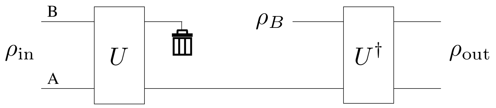
Refer to caption — Figure 1: Quantum Autoencoder: We use $U$ to compress the input state $\rho_{\text{in}}$ into the reduced Hilbert space $\mathcal{H}_{A}$ , and use the state $\rho_{B}$ of the fresh qubits in $\mathcal{H}_{B}$ to decompress the data by applying the unitary $U^{\dagger}$ to generate the output state $\rho_{\text{out}}$ .

In this setup, we apply a parameterized unitary $U$ to the input state $\rho_{\text{in}}$ and perform the partial trace over $\mathcal{H}_{B}$ to compress the quantum data into the latent Hilbert space $\mathcal{H}_{A}$ . Then, we use the fresh qubits prepared in the state $\rho_{B}\in\mathcal{B}(\mathcal{H}_{B})$ to decompress the data by applying the unitary $U^{\dagger}$ to generate the output state $\rho_{\text{out}}$ . In this case, we have

\displaystyle\rho_{\text{out}}=\Phi(\rho_{\text{in}})\equiv U^{\dagger}\left({\rm Tr}_{B}\left[U\rho_{\text{in}}U^{\dagger}\right]\otimes\rho_{B}\right)U\,.

(15)

To discuss the Jarzynski-like equality, it is convenient to define the compressed states

	$\displaystyle\rho_{A}$	$\displaystyle\equiv{\rm Tr}_{B}\left[U\rho_{\text{in}}U^{\dagger}\right]$		(16)
	$\displaystyle\rho_{A}^{(i)}$	$\displaystyle\equiv{\rm Tr}_{B}\left[U\|p_{i}\rangle\!\langle p_{i}\|U^{\dagger}\right]\,.$		(17)

Therefore, we can write $\rho_{A}=\sum_{i=1}^{d}p_{i}\rho_{A}^{(i)}$ , so that we have $\text{supp}(\rho_{A}^{(i)})\subseteq\text{supp}(\rho_{A})$ .

Given this setup above, we can relate $L_{\text{otm}}$ to the classical information transmission and the cost function in QAE, which demonstrates the roles of the quantum cross entropy in quantum communications and quantum machine learning in the framework of QAE protocol.

Let us first derive the expression of $L_{\text{otm}}$ in QAE. From Eq. (15), we have

\displaystyle C(\Phi(|p_{i}\rangle\!\langle p_{i}|),\rho_{\text{out}})=S(\rho_{B})+C(\rho_{A}^{(i)},\rho_{A})\,.

(18)

Therefore, we can write

\displaystyle\langle e^{-\sigma}\rangle_{\widetilde{P}}=e^{-S(\rho_{B})}\sum_{i=1}^{r}e^{-C(\rho_{A}^{(i)},\rho_{A})}\,,

(19)

so that $L_{\text{otm}}$ is given by

\displaystyle L_{\text{otm}}=S(\rho_{B})-\ln\left(\sum_{i=1}^{r}e^{-C(\rho_{A}^{(i)},\rho_{A})}\right)\,.

(20)

An important observation is that $\langle e^{-\sigma}\rangle_{\widetilde{P}}$ includes two terms which characterize the protocols of the QAE. One is the von-Neumann entropy $S(\rho_{B})$ , which is the informational contribution from the state preparation protocol in the fresh-qubit system $\mathcal{H}_{B}$ . The other one is associated with the quantum cross entropy $C(\rho_{A}^{(i)},\rho_{A})$ with respect to the latent Hilbert space $\mathcal{H}_{A}$ . This quantity can be regarded as a term characterizing the compression protocol of the QAE. In the following, we explore the roles of the quantum cross entropy in the quantum communications and quantum machine learning from the relation of the lower bound $L_{\text{otm}}$ to the loss of Holevo information and the global cost function of the QAE.

III.1.1 Relation to the loss of Holevo information in QAE

Here, we explore the relation between $L_{\text{otm}}$ and the entropic disturbance. Entropic disturbance is the loss of Holevo information through a given quantum channel $\Phi$ Buscemi and Horodecki 2009; Buscemi et al. 2016. Hence, it quantifies the loss of the maximum amount of classical information transmittable through the quantum channel. In Ref. Buscemi et al. 2016, a lower bound on $\Delta\chi$ was derived. Here, for a given quantum channel $\Phi$ , we provide an upper bound on the entropic disturbance by using $L_{\text{otm}}$ to provide a operational meaning to the quantum cross entropy in terms of classical information transmission.

The entropic disturbance is defined as follows. Let $\mathcal{L}\equiv\{p_{i},\rho_{i}\}_{i=1}^{r}$ denote an ensemble of input state $\rho_{\text{in}}\equiv\sum_{i=1}^{r}p_{i}\rho_{i}$ and $\Phi(\mathcal{L})\equiv\{p_{i},\Phi(\rho_{i})\}_{i=1}^{r}$ denote the ensemble of output state $\rho_{\text{out}}\equiv\Phi(\rho_{\text{in}})=\sum_{i=1}^{r}p_{i}\Phi(\rho_{i})$ . Entropic disturbance is defined as $\Delta\chi\equiv\chi(\mathcal{L})-\chi(\Phi(\mathcal{L}))$ , where $\chi(\mathcal{L})\equiv S(\rho_{\text{in}})-\sum_{i=1}^{r}p_{i}S(\rho_{i})$ and $\chi(\Phi(\mathcal{L}))\equiv S(\rho_{\text{out}})-\sum_{i=1}^{r}p_{i}S(\Phi(\rho_{i}))$ are the Holevo information of $\rho_{\text{in}}$ and $\rho_{\text{out}}$ , respectively. In our case, we have $\rho_{i}=|p_{i}\rangle\!\langle p_{i}|$ , so that $S(\rho_{i})=S(|p_{i}\rangle\!\langle p_{i}|)=0$ . Therefore, due to $\Delta S\geqslant L_{\text{otm}}$ and Eq. (8), we can obtain

\displaystyle\Delta\chi\leqslant\ln\left(\sum_{i=1}^{r}e^{-C(\Phi(|p_{i}\rangle\!\langle p_{i}|),\rho_{\text{out}})}\right)+\sum_{i=1}^{r}p_{i}S(\Phi(|p_{i}\rangle\!\langle p_{i}|)),

(21)

which shows that the upper bound of the entropic disturbance can be characterized by the quantum cross entropy. ³³ 3 When $\Phi$ is a unitary operation, we have $L_{\text{otm}}=0$ and $S(\Phi(|p_{i}\rangle\!\langle p_{i}|))=0$ . Because the entropic disturbance is invariant under the unitary operation $\Delta\chi=0$ , we can say that the upper bound is tight for the unitary operation..

Now, let us consider the case of QAE, in which $\Phi$ satisfies Eq. (15). Due to $S(\Phi(|p_{i}\rangle\!\langle p_{i}|))=S(\rho_{A}^{(i)})+S(\rho_{B})$ , we have $\sum_{i=1}^{r}p_{i}S(\Phi(|p_{i}\rangle\!\langle p_{i}|))=\sum_{i=1}^{r}p_{i}S(\rho_{A}^{(i)})+S(\rho_{B})$ , so that the upper bound on $\Delta\chi$ in QAE is given by

\displaystyle\Delta\chi\leqslant\sum_{i=1}^{r}p_{i}S(\rho_{A}^{(i)})+\ln\left(\sum_{i=1}^{r}e^{-C(\rho_{A}^{(i)},\rho_{A})}\right)\,.

(22)

Therefore, the information and the quantum cross entropy of the compressed states contributes to setting an upper bound on entropic disturbance of in the QAE protocol. Also, note that for the QAE, $\Delta\chi$ can be explicitly written as

\displaystyle\Delta\chi=S(\rho_{\text{in}})-S(\rho_{A})-\sum_{i=1}^{r}p_{i}S(\rho_{A}^{(i)})\,,

(23)

which implies that the loss of the maximum amount of classical information in the QAE protocol is independent of the choice of $\rho_{B}$ but strictly dependent on the compressed and input state.

III.1.2 Relation to the global cost function of QAE

The lower bound $L_{\text{otm}}$ can be also related to the performance of the QAE, which can be characterized by its global cost function. The cost function of the QAE is well-defined when the fresh-qubit state $\rho_{B}$ is a pure state

\displaystyle\rho_{B}=|\psi\rangle\!\langle\psi|\,.

(24)

In this case, from Eq. (20) and $S(\rho_{B})=S(|\psi\rangle\!\langle\psi|)=0$ . we have

\displaystyle L_{\text{otm}}=-\ln\left(\sum_{i=1}^{r}e^{-C(\rho_{A}^{(i)},\rho_{A})}\right)\,.

(25)

Let $\eta_{B}$ denote the reduced state $\eta_{B}\equiv{\rm Tr}_{A}[U\rho_{\text{in}}U^{\dagger}]$ . Then, from Refs. Romero et al. 2017; Cerezo et al. 2021b, the global cost function $\mathscr{C}$ can be given by

\displaystyle\mathscr{C}\equiv 1-\langle\psi\hskip 1.0pt|\eta_{B}|\hskip 1.0pt\psi\rangle\,,

(26)

which satisfies $0\leqslant\mathscr{C}\leqslant 1$ . The ultimate goal of this protocol is to find a optimal unitary $U_{*}$ to realize $\rho_{\text{in}}=\rho_{\text{out}}$ . In this optimal case, the global cost function is $\mathscr{C}=0$ . Then, by using $d_{B}$ the dimension of $\mathcal{H}_{B}$ and the global cost function, we can obtain the following inequality (See Appendix. A for the proof)

\displaystyle L_{\text{otm}}\leqslant\Delta S\leqslant 2\ln\left(\sqrt{1-\mathscr{C}}+\sqrt{(d_{B}-1)\mathscr{C}}\right)\,.

(27)

From Eq. (25), we can finally obtain

\displaystyle\sum_{i=1}^{r}e^{-C(\rho_{A}^{(i)},\rho_{A})}\geqslant\left(\frac{1}{\sqrt{1-\mathscr{C}}+\sqrt{(d_{B}-1)\mathscr{C}}}\right)^{2}\,,

(28)

which shows that the quantum cross entropy plays a role as an informational contribution of the compressed state to the performance of the QAE protocol. Here, note that, due to $0\leqslant\mathscr{C}\leqslant 1$ , we have $0\leqslant 2\ln\left(\sqrt{1-\mathscr{C}}+\sqrt{(d_{B}-1)\mathscr{C}}\right)\leqslant\ln(d_{B})$ , where $\mathscr{C}=0$ (i.e., $\eta_{B}=|\psi\rangle\!\langle\psi|$ ) leads to the minimum, and $\mathscr{C}=1-1/d_{B}$ (i.e., $\eta_{B}=\openone_{B}/d_{B}$ ) leads to the maximum.

We can also check the consistency of Eq. (27) by considering the optimal case. The optimal unitary $U_{*}$ is a disentangling gate Ma et al. 2020, so that $U_{*}$ satisfies

\displaystyle\begin{split}U_{*}\rho_{\text{in}}U_{*}^{\dagger}&=\rho_{A}\otimes|\psi\rangle\!\langle\psi|\\ U_{*}|p_{i}\rangle\!\langle p_{i}|U_{*}^{\dagger}&=\rho_{A}^{(i)}\otimes|\psi\rangle\!\langle\psi|\,.\end{split}

(29)

Then, by using the unitary invariance of the quantum cross entropy, we obtain

\displaystyle\begin{split}C\left(\rho_{A}^{(i)},\rho_{A}\right)&=C\left(\rho_{A}^{(i)}\otimes|\psi\rangle\!\langle\psi|,\rho_{A}\otimes|\psi\rangle\!\langle\psi|\right)\\ &=C(|p_{i}\rangle\!\langle p_{i}|,\rho_{\text{in}})\\ &=-\ln p_{i}\,.\end{split}

(30)

In this way, we have $L_{\text{otm}}=0$ . By definition, in the optimal case, we have $\mathscr{C}=0$ ; therefore, $\ln\left(\sqrt{1-\mathscr{C}}+\sqrt{(d_{B}-1)\mathscr{C}}\right)=0$ . From $L_{\text{otm}}\leqslant\Delta S\leqslant 2\ln\left(\sqrt{1-\mathscr{C}}+\sqrt{(d_{B}-1)\mathscr{C}}\right)$ , we get the expected result $\Delta S=0$ for the optimal unitary case.

III.2 Maximum Available Work Theorem

For the second example, we explore the role of quantum cross entropy in work extraction from the quantum thermodynamic systems by from the relation between $L_{\text{otm}}$ and the maximum available work theorem Deffner 2017.

In Ref. Deffner 2017, a generic quantum thermodynamic system is regarded as a tripartite system composed of the system, work reservoir and heat bath. In this setup, the work $\langle W\rangle$ , the internal energy change of the system $\Delta E_{s}$ and the internal energy change of the heat bath $\Delta E_{b}$ satisfy the first law of thermodynamics $\Delta E_{s}+\Delta E_{b}=\langle W\rangle$ . Also, when $\Delta S$ and $\Delta S_{b}$ denote the von-Neumann entropy change of the system and heat bath, respectively, the second law of thermodynamics states $\Delta S+\Delta S_{b}\geqslant 0$ . Because the heat reservoir is so large, which can be regarded as being always in equilibrium at inverse temperature $\beta$ , we can write $\Delta S_{b}=\beta\Delta E_{b}$ . Then, the maximum available work theorem states

\displaystyle\langle W\rangle\geqslant\Delta E_{s}-\beta^{-1}\Delta S\equiv\Delta\mathcal{E}\,,

(31)

where $\mathcal{E}$ is called exergy or availability, which quantifies the maximally available work.

In this setup, from Theorem. 1, we can obtain the upper bound on the exergy $\Delta\mathcal{E}$ as

\displaystyle\Delta\mathcal{E}\leqslant\Delta E_{s}+\beta^{-1}\ln\left(\sum_{i=1}^{r}e^{-C(\Phi(|p_{i}\rangle\!\langle p_{i}|),\rho_{\text{out}})}\right)\,.

(32)

This demonstrates the informational contribution of the quantum cross entropy in extracting maximally available work in the quantum thermodynamic systems. If there is no work reservoir, i.e., $\langle W\rangle=0$ , the corresponding maximum available work theorem becomes $\Delta S\geqslant-\beta\Delta E_{b}$ . However, when the system undergoes the energy-emitting process ( $\Delta E_{b}\geqslant 0$ ) described by a unital evolution, from Corollary 1, we have a tighter bound as

\displaystyle\Delta S\geqslant L_{\text{otm}}\geqslant-\beta\Delta E_{b}\,.

(33)

A good example of the energy-emitting unital evolution is the spin-boson model Schlosshauer 2007. Let us consider a system $\mathcal{H}_{s}$ initially prepared in $\rho_{\text{in}}$ coupled to a heat bath $\mathcal{H}_{b}$ , whose initial state is prepared in the Gibbs state

\displaystyle\rho_{b}^{\text{eq}}\equiv\frac{e^{-\beta H_{b}}}{Z}\,,

(34)

where $Z\equiv{\rm Tr}\left[e^{-\beta H_{b}}\right]$ is the canonical partition function with inverse temperature $\beta$ and $H_{b}$ the time-independent bare Hamiltonian of the bath. Then, when $\Phi$ is a thermal operation Sagawa 2012; Ng and Woods 2018; Goold et al. 2016 from $t=0$ to $t=\tau$ ,

\displaystyle\rho_{\text{out}}=\Phi(\rho_{\text{in}})={\rm Tr}_{b}\left[U_{\tau}(\rho_{\text{in}}\otimes\rho_{b}^{\text{eq}})U_{\tau}^{\dagger}\right]\,.

(35)

In the quantum thermodynamic setup of the spin-boson model, $\mathcal{H}_{s}$ and $\mathcal{H}_{b}$ usually describes a two-level atomic system and the bosonic heat bath, respectively (See Fig. 2), and the atomic system in Eq. (35) undergoes the dephasing process, which is described by a unital map.

This model can be descried by the following time-independent Hamiltonian (we set $\hbar=1$ )

\displaystyle H=\frac{\omega_{0}}{2}\sigma_{z}+H_{b}+\sigma_{z}\otimes\sum_{k}(g_{k}a_{k}+g_{k}^{*}a_{k}^{\dagger}),

(36)

where

\displaystyle H_{b}\equiv\sum_{k}\omega_{k}a_{k}^{\dagger}a_{k}

(37)

is the bare Hamiltonian of the boson fields, and $\sigma_{z}\equiv\rm diag(1,-1)$ is the Pauli’s Z operator acting on the atom. $\omega_{0}$ and $\omega_{k}$ are the angular frequencies of the atom and the $k$ -th boson mode, and $g_{k}$ denotes the coupling strength between the atom and the $k$ -th boson mode. Here, in general $g_{k}$ is a complex number, and $g_{k}^{*}$ denotes the complex conjugate of $g_{k}$ . Also, $a_{k}(a_{k}^{\dagger})$ is the annihilation (creation) operator of $k$ -th mode of the boson fields. The Hamiltonian Eq. (36) describes an interaction between atom and boson fields with multiple modes, which leads to the dephasing process of the atomic system. In interaction picture, we have

\displaystyle H(t)=\sigma_{z}\otimes\sum_{k}(g_{k}a_{k}e^{-i\omega_{k}t}+g_{k}^{*}a_{k}^{\dagger}e^{+i\omega_{k}t}).

(38)

During the evolution from $t=0$ to $t=\tau$ , the internal energy change of the heat bath becomes (See Appendix. B for the proof)

\displaystyle\begin{split}\Delta E_{b}&\equiv{\rm Tr}\left[U_{\tau}(\rho_{\text{in}}\otimes\rho_{b}^{\text{eq}})U_{\tau}^{\dagger}H_{b}\right]-{\rm Tr}\left[\rho_{b}^{\text{eq}}H_{b}\right]\\ &=\sum_{k}\omega_{k}|g_{k}|^{2}\left(\frac{\sin(\omega_{k}\tau/2)}{\omega_{k}/2}\right)^{2}\geqslant 0\,,\end{split}

(39)

which shows that the system undergoes the energy-emitting process, which can be verified from the energy conservation of the total system. Considering the noise spectral density $J(\omega)=\sum_{k}|g_{k}|^{2}\omega\delta(\omega-\omega_{k})$ , we can obtain

\displaystyle\Delta E_{b}=\int_{-\infty}^{\infty}J(\omega)\left(\frac{\sin(\omega\tau/2)}{\omega/2}\right)^{2}d\omega\,.

(40)

Since we have $\lim_{\tau\to\infty}\frac{\sin(\omega\tau/2)}{\omega/2}=\delta\left(\omega/2\right)=2\delta(\omega)$ , where we used the relation $\lim_{\tau\to\infty}\left(\tau\frac{\sin(\omega\tau)}{\omega\tau}\right)=\delta(\omega)$ , we obtain

\displaystyle\lim_{\tau\to\infty}\Delta E_{b}=\int_{-\infty}^{\infty}4J(\omega)\delta^{2}(\omega)d\omega=4J(0)\delta(0)=0\,.

(41)

This is intuitively consistent because there will be no energy exchange between a small system and a large bath for the dephasing process at time $\tau\to\infty$ .

In the spin-boson model, the work reservoir is not taken into account. Therefore, we have $\Delta S\geqslant-\beta\Delta E_{b}$ . Since the two-level atom undergoes the unital evolution, the total information production has to be $\Delta S\geqslant 0$ . However, from Eq. (39), we have $-\beta\Delta E_{b}\leqslant 0$ , which shows that the lower bound in the maximum available work theorem for the spin-boson model is not tight enough. Instead, from Corollary. 1, we can find that $L_{\text{otm}}$ is the tighter bound as demonstrated in Eq. (33). Because $L_{\text{otm}}$ is characterized by the quantum cross entropy, the quantum cross entropy becomes a more meaningful quantity to characterize the quantum process of a system induced from its interaction with a heat bath.

IV Conclusion

In conclusion, we have proposed a distribution of an information production for a quantum state of arbitrary rank and a quantum channel by adopting the one-time measurement scheme. The derived Jarzynski-like equality and the lower bound on the total information production are characterized by the quantum cross entropy, which further enables one to explore the roles of quantum cross entropy in quantum communications, quantum machine learning and quantum thermodynamics. By focusing on the quantum autoencoder, we have explored the informational contributions of the quantum cross entropy of the compressed states to the loss of the maximum classical information transmittable through the circuit and the performance of the protocol characterized by the global cost function. We have also demonstrated the application of our result in the quantum thermodynamics by exploring relation between the quantum cross entropy and the maximum available work theorem. Our result can provide insights of the quantum cross entropy to assist designing quantum information processing protocols which utilize the quantum cross entropy as a resource to achieve some tasks. As a valuable future direction, we will explore reverse process in the OTM scheme, which still remains open.

Acknowledgements

We would like to thank Sebastian Deffner, Hailan Ma, Yuanlong Wang, and Marco Cerezo for helpful discussions. This work is supported by NSF: Proposal 2036347 (STTR Phase 1). A.S. was supported by the internal R&D from Aliro Technologies, Inc. Now, he is supported by the startup package from University of Massachusetts Boston. N.Y. is supported by MEXT Quantum Leap Flagship Program Grants No. JPMXS0118067285 and No. JPMXS0120319794. T.J.H is supported by the graduate study program at University of Massachusetts Boston. Work by P.N. is supported by the NSF RAISE-QAC-QSA, Grant No. DMR-2037783 and the Department of Energy, Office of Basic Energy Sciences Grant DE-SC0019215.

Appendix

Appendix A Proof of Eq. (27)

Here, we provide a detailed proof of Eq. (27). First, by using the cost function $\mathscr{C}$ , we can obtain an upper bound on $\Delta S$ . From

\displaystyle\rho_{\text{out}}=U^{\dagger}\left(\rho_{A}\otimes|\psi\rangle\!\langle\psi|\right)U

(1)

with $\rho_{A}\equiv{\rm Tr}_{B}[U\rho_{\text{in}}U^{\dagger}]$ , because the von-Neumann entropy is unitarily invariant, we have

\displaystyle\begin{split}S(\rho_{\text{out}})&=S(\rho_{A}\otimes|\psi\rangle\!\langle\psi|)=S(\rho_{A})\\ S(\rho_{\text{in}})&=S(U\rho_{\text{in}}U^{\dagger})\,,\end{split}

(2)

which leads to

\displaystyle\Delta S=S(\rho_{A})-S(U\rho_{\text{in}}U^{\dagger})\,.

(3)

Because $\eta_{B}\equiv{\rm Tr}_{A}\left[U\rho_{\text{in}}U^{\dagger}\right]$ , from Araki-Lieb inequality Araki and Lieb 1970

\displaystyle|S(\rho_{A})-S(\eta_{B})|\leqslant S(U\rho_{\text{in}}U^{\dagger})\,,

(4)

we have

\displaystyle\Delta S\leqslant S(\eta_{B})\,.

(5)

By using $d_{B}$ the dimension of the Hilbert space $\mathcal{H}_{B}$ , $S(\eta_{B})$ can be upper bounded as

\displaystyle\begin{split}S(\eta_{B})&=\ln(d_{B})-S\left(\eta_{B}\,\Big|\Big|\,\frac{\openone_{B}}{d_{B}}\right)\\ &\leqslant\ln(d_{B})-S_{\min}\left(\eta_{B}\,\Big|\Big|\,\frac{\openone_{B}}{d_{B}}\right)\,,\end{split}

(6)

where

\displaystyle S_{\min}(\rho_{1}||\rho_{2})\equiv-\ln\left(F[\rho_{1},\rho_{2}]\right)

(7)

denotes the sandwiched min relative entropy of $\rho_{1}$ with respect to $\rho_{2}$ Wilde et al. 2014; Beigi 2013; Sagawa 2020 with the standard quantum fidelity defined as

\displaystyle F[\rho_{1},\rho_{2}]\equiv\left({\rm Tr}\left[\sqrt{\rho_{1}^{1/2}\rho_{2}\rho_{1}^{1/2}}\right]\right)^{2}\,.

(8)

Therefore, we have

\displaystyle S(\eta_{B})\leqslant\ln\left(d_{B}F\left[\eta_{B},\frac{\openone_{B}}{d_{B}}\right]\right)\,.

(9)

Here, we consider so-called generalized quantum fidelity Tomamichel et al. 2010; Tomamichel 2015; Cappellini et al. 2007; Cerezo et al. 2020, which is defined as

\displaystyle\widetilde{F}\left[\sigma_{1},\sigma_{2}\right]\equiv\left(\sqrt{F\left[\sigma_{1},\sigma_{2}\right]}+\sqrt{(1-{\rm Tr}\left[\sigma_{1}\right])(1-{\rm Tr}\left[\sigma_{2}\right])}\right)^{2}.

(10)

Here, note that $\sigma_{1}$ and $\sigma_{2}$ are the sub-normalized states i.e. $0\leqslant{\rm Tr}\left[\sigma_{1}\right]\leqslant 1$ and $0\leqslant{\rm Tr}[\sigma_{2}]\leqslant 1$ . Because applying the projection operator $|\psi\rangle\!\langle\psi|$ is described by the completely positive trace non-increasing (CPTNI) map Cerezo et al. 2020, from the monotonicity of the generalized quantum fidelity under the CPTNI maps Tomamichel et al. 2010; Tomamichel 2015; Cappellini et al. 2007; Cerezo et al. 2020, we have

\displaystyle\begin{split}F\left[\eta_{B},\frac{\openone_{B}}{d_{B}}\right]&=\widetilde{F}\left[\eta_{B},\frac{\openone_{B}}{d_{B}}\right]\\ &\leqslant\widetilde{F}\left[|\psi\rangle\!\langle\psi|\eta_{B}|\psi\rangle\!\langle\psi|,\frac{1}{d_{B}}|\psi\rangle\!\langle\psi|\right]\,.\end{split}

(11)

Since we have

\displaystyle\begin{split}\widetilde{F}&\left[|\psi\rangle\!\langle\psi|\eta_{B}|\psi\rangle\!\langle\psi|,\frac{1}{d_{B}}|\psi\rangle\!\langle\psi|\right]\\ &=\left(\sqrt{\frac{1-\mathscr{C}}{d_{B}}}+\sqrt{\mathscr{C}\left(1-\frac{1}{d_{B}}\right)}\right)^{2}\,,\end{split}

(12)

we can obtain

\displaystyle\Delta S\leqslant S(\eta_{B})\leqslant 2\ln\left(\sqrt{1-\mathscr{C}}+\sqrt{(d_{B}-1)\mathscr{C}}\right)\,,

(13)

which states that the information production in quantum autoencoder with pure fresh-qubit state can be upper bounded by using $\mathscr{C}$ . Therefore, from Theorem. 1, we can finally arrive at Eq. (27)

\displaystyle L_{\text{otm}}\leqslant\Delta S\leqslant 2\ln\left(\sqrt{1-\mathscr{C}}+\sqrt{(d_{B}-1)\mathscr{C}}\right)\,.

(14)

Appendix B Proof of Eq. (39)

We demonstrate the detailed proof of Eq. (39) based on Refs. Cappellaro 2012; Sone et al. 2020. The Hamiltonian of the spin-boson model is

\displaystyle H=\frac{\omega_{0}}{2}\sigma_{z}+H_{b}+\sigma_{z}\otimes\sum_{k}(g_{k}a_{k}+g_{k}^{*}a_{k}^{\dagger})\,,

(15)

where we define $\sigma_{z}\equiv\begin{pmatrix}1&0\\ 0&-1\end{pmatrix}$ and $a_{k}(a_{k}^{\dagger})$ as the annihilation (creation) operator of $k$ -th mode of the boson heat bath. The annihilation and creation operators satisfy the commutation relation

\displaystyle[a_{k},a_{k^{\prime}}^{\dagger}]=\delta_{kk^{\prime}},~[a_{k},a_{k^{\prime}}]=[a_{k}^{\dagger},a_{k^{\prime}}^{\dagger}]=0\,.

(16)

Also, $H_{b}$ is defined as

\displaystyle H_{b}\equiv\sum_{k}\omega_{k}a_{k}^{\dagger}a_{k}\,.

(17)

Then, the Hamiltonian in the interaction picture becomes

\displaystyle H(t)=\sigma_{z}\otimes\sum_{k}(g_{k}a_{k}e^{-i\omega_{k}t}+g_{k}^{*}a_{k}^{\dagger}e^{i\omega_{k}t})\,.

(18)

Using Magnus expansion, the propagator becomes

\displaystyle U_{t}=\exp\left[-it(\overline{H}_{0}+\overline{H}_{1})\right],

(19)

where the higher terms are vanishing because $[H(t_{1}),H(t_{2})]$ becomes just a number (See Eq. (24)). Here, we define

\displaystyle\overline{H}_{0}\equiv\frac{1}{t}\int_{0}^{t}H(t_{1})dt_{1}

(20)

and

\displaystyle\overline{H}_{1}\equiv-\frac{i}{2t}\int_{0}^{t}dt_{1}\int_{0}^{t_{1}}dt_{2}[H(t_{1}),H(t_{2})].

(21)

More explicitly, $\overline{H}_{0}$ can be written as

\displaystyle\overline{H}_{0}=\sigma_{z}\otimes\sum_{k}\left(G_{k}(t)a_{k}+G^{*}(t)a_{k}^{\dagger}\right),

(22)

where

\displaystyle G_{k}(t)\equiv g_{k}\frac{\sin(\omega_{k}t/2)}{\omega_{k}t/2}e^{-i\omega_{k}t/2}.

(23)

For $\overline{H}_{1}$ , because we have

\displaystyle[H(t_{1}),H(t_{2})]=-2i\sum_{k}|g_{k}|^{2}\sin\left(\omega_{k}(t_{1}-t_{2})\right)\,

(24)

and

\displaystyle\begin{split}\int_{0}^{t}dt_{1}\int_{0}^{t_{1}}&dt_{2}\sin\left(\omega_{k}(t_{1}-t_{2})\right)\\ &=\frac{1}{\omega_{k}}\left(t-\frac{1}{\omega_{k}}\sin(\omega_{k}t)\right)\,,\end{split}

(25)

we can write

\displaystyle\overline{H}_{1}=-\sum_{k}\frac{|g_{k}|^{2}}{\omega_{k}}\left(1-\frac{\sin(\omega_{k}t)}{\omega_{k}t}\right)\in\mathbb{R}\,,

(26)

which is just a real number.

Therefore, from Eqs. (19), (22), and (26), the propagator becomes

\displaystyle U_{t}=\exp\left[-it\sum_{k}\left(\sigma_{z}\otimes(G_{k}(t)a_{k}+G_{k}^{*}(t)a_{k}^{\dagger})\right)\right]e^{-it\overline{H}_{1}}\,.

(27)

With this propagator, due to

\displaystyle\begin{split}\!\!\!\!\left[\sum_{k^{\prime}}\sigma_{z}\otimes(G_{k^{\prime}}(t)a_{k^{\prime}}+G_{k^{\prime}}^{*}(t)a_{k^{\prime}}^{\dagger}),a_{k}\right]&\!=\!-G_{k}^{*}(t)\sigma_{z}\\ \!\!\!\!\left[\sum_{k^{\prime}}\sigma_{z}\otimes(G_{k^{\prime}}(t)a_{k^{\prime}}+G_{k^{\prime}}^{*}(t)a_{k^{\prime}}^{\dagger}),a_{k}^{\dagger}\right]&\!=\!G_{k}(t)\sigma_{z}\,,\end{split}

(28)

from Baker-Hausdorff-Campbell’s formula, we have

\displaystyle\begin{split}U_{t}^{\dagger}a_{k}U_{t}&=a_{k}-itG_{k}^{*}(t)\sigma_{z}\\ U_{t}^{\dagger}a_{k}^{\dagger}U_{t}&=a_{k}^{\dagger}+itG_{k}(t)\sigma_{z}\,.\end{split}

(29)

Therefore, we can write

\displaystyle\begin{split}\!\!\!\!U_{t}^{\dagger}H_{b}U_{t}=&\sum_{k}\omega_{k}\left(U_{t}^{\dagger}a_{k}^{\dagger}U_{t}\right)\left(U_{t}^{\dagger}a_{k}U_{t}\right)\\ =&H_{b}+it\sum_{k}\omega_{k}\sigma_{z}\otimes(G_{k}(t)a_{k}-G_{k}^{*}(t)a_{k}^{\dagger})\\ &+\sum_{k}\omega_{k}|G_{k}(t)|^{2}t^{2}\,.\end{split}

(30)

Let $\rho_{\text{in}}$ be the input state of the system with a rank $r$ , and the initial state of the boson heat bath be the Gibbs state

\displaystyle\rho_{b}^{\text{eq}}=\frac{e^{-\beta H_{b}}}{Z}\,.

(31)

Note that, with $a_{k}$ and $a_{k}^{\dagger}$ , for all $k$ , we have

\displaystyle{\rm Tr}\left[\rho_{b}^{\text{eq}}a_{k}\right]={\rm Tr}\left[\rho_{b}^{\text{eq}}a_{k}^{\dagger}\right]=0\,.

(32)

We assume that the two-level atomic system and bosonic field are initially decoupled. Therefore, the initial state of the total system is $\rho_{\text{in}}\otimes\rho_{b}^{\text{eq}}$ , so that the evolution of the atomic system from $t=0$ to $t=\tau$ is described by the following thermal operation

\displaystyle\rho_{\text{out}}=\Phi(\rho_{\text{in}})={\rm Tr}_{b}\left[U_{\tau}(\rho_{\text{in}}\otimes\rho_{b}^{\text{eq}})U_{\tau}^{\dagger}\right]\,.

(33)

The internal energy change of the heat bath during the evolution can be defined as the difference in the average energy of the heat bath at $t=\tau$ and $t=0$

\displaystyle\Delta E_{b}\equiv{\rm Tr}\left[U_{\tau}(\rho_{\text{in}}\otimes\rho_{b}^{\text{eq}})U_{\tau}^{\dagger}H_{b}\right]-{\rm Tr}\left[\rho_{b}^{\text{eq}}H_{b}\right]\,.

(34)

From Eqs. (23), (30) and (32), $\Delta E_{b}$ can be explicitly written as

\displaystyle\Delta E_{b}=\sum_{k}\omega_{k}|g_{k}|^{2}\left(\frac{\sin\left(\omega_{k}\tau/2\right)}{\omega_{k}/2}\right)^{2}\geqslant 0\,.

(35)

Appendix C Second-law-like Inequality Involving Guessed Heat

The information production distribution $\widetilde{P}(\sigma)$ can be related to the distribution of the internal energy difference in OTM scheme $\widetilde{P}(\Delta E_{s})$ in a very special case, which leads to a second-law-like inequality involving the guessed heat introduced in Ref. Sone et al. 2020. Let $H_{s}(t)$ be the system’s bare Hamiltonian, which is time-dependent. Also, suppose that the system is initially decoupled from the heat bath, which is initially prepared in a Gibbs state

\displaystyle\rho_{b}^{\text{eq}}=\frac{e^{-\beta H_{b}}}{Z_{b}}\,,

(36)

where $H_{b}$ is the bath’s bare Hamiltonian, which is time-independent. Here, $Z_{b}\equiv{\rm Tr}\left[e^{-\beta H_{b}}\right]$ is the partition function defined by $H_{b}$ . Let $H_{\text{int}}$ be the interaction Hamiltonian. Then, the unitary operator $U_{t}$ describing the time evolution of the total system follows the Schrödinger’s equation $\partial_{t}U_{t}=-i(H_{s}(t)+H_{b}+H_{\text{int}})U_{t}$ with $U_{0}\equiv\openone$ . Evolving the total system from $t=0$ to $t=\tau$ and focusing on the system alone, we have

\displaystyle\rho_{\text{out}}=\Phi(\rho_{\text{in}})={\rm Tr}_{b}\left[U_{\tau}(\rho_{\text{in}}\otimes\rho_{b}^{\text{eq}})U_{\tau}^{\dagger}\right]\,.

(37)

Let $\{E_{i},|E_{i}\rangle\}_{i=1}^{d}$ be an eigensystem of $H_{s}(0)$ . When we have

\displaystyle\begin{split}\rho_{\text{in}}&=\rho_{s}^{\text{eq}}(0)\equiv\frac{e^{-\beta H_{s}(0)}}{Z_{0}}\\ \rho_{\text{out}}&=\rho_{s}^{\text{eq}}(\tau)\equiv\frac{e^{-\beta H_{s}(\tau)}}{Z_{\tau}}\,,\end{split}

(38)

where $Z_{0}\equiv{\rm Tr}\left[e^{-\beta H_{s}(0)}\right]$ and $Z_{\tau}\equiv{\rm Tr}\left[e^{-\beta H_{s}(\tau)}\right]$ are the partition functions defined by $H_{s}(0)$ and $H_{s}(\tau)$ , respectively, from Eq. (4), the information production distribution in the OTM scheme becomes

\displaystyle\widetilde{P}(\sigma)=\frac{1}{\beta}\sum_{i=1}^{d}\frac{e^{-\beta E_{i}}}{Z_{0}}\delta\left(\frac{\sigma}{\beta}+\Delta F-\Delta\widetilde{E}(E_{i})\right)\,,

(39)

where

\displaystyle\Delta\widetilde{E}(E_{i})\equiv{\rm Tr}\left[\Phi(|E_{i}\rangle\!\langle E_{i}|)H_{s}(\tau)\right]-E_{i}\,,

(40)

and

\displaystyle\Delta F\equiv-\beta^{-1}\ln\left(\frac{Z_{\tau}}{Z_{0}}\right)

(41)

is the equilibrium Helmholtz free energy difference. From Ref. Sone et al. 2020, $\widetilde{P}(\Delta E_{s})$ is given by

\displaystyle\widetilde{P}(\Delta E_{s})\!=\!\sum_{i=1}^{d}\frac{e^{-\beta E_{i}}}{Z_{0}}\delta\left(\Delta E_{s}-\Delta\widetilde{E}(E_{i})\right)\,.

(42)

Therefore, we can write

\displaystyle\widetilde{P}(\Delta E_{s})=\beta\widetilde{P}(\sigma)

(43)

with the random variable $\sigma$ being

\displaystyle\sigma=\beta(\Delta E_{s}-\Delta F)\,.

(44)

Following Ref. Sone et al. 2020, we have

\displaystyle\langle e^{-\beta\Delta E_{s}}\rangle_{\widetilde{P}}=e^{-\beta\Delta F}e^{-\beta\langle\widetilde{Q}\rangle_{b}}e^{-S(\Theta_{sb}(\tau)||\rho_{s}^{\text{eq}}(\tau)\otimes\rho_{b}^{\text{eq}})}\,,

(45)

where

\displaystyle\Theta_{sb}(\tau)\equiv\sum_{i=1}^{d}\frac{e^{-\beta{\rm Tr}\left[\Phi(|E_{i}\rangle\!\langle E_{i}|)H_{s}(\tau)\right]}}{\widetilde{Z}_{\tau}}U_{\tau}\left(|E_{i}\rangle\!\langle E_{i}|\otimes\rho_{b}^{\text{eq}}\right)U_{\tau}^{\dagger}\,

(46)

is called “guessed state", and $\langle\widetilde{Q}\rangle_{b}$ is a heat-like quantity called “guessed heat" defined as

\displaystyle\langle\widetilde{Q}\rangle_{b}\equiv{\rm Tr}\left[H_{b}\rho_{b}^{\text{eq}}\right]-{\rm Tr}\left[H_{b}\Theta_{sb}(\tau)\right]\,.

(47)

This heat-like quantity describes an energy dissipation from the heat bath as if its final state is ${\rm Tr}_{s}\left[\Theta_{sb}(\tau)\right]$ the reduced state of the guessed state. From Eq. (43) and (44), we can obtain

\displaystyle\langle e^{-\beta\Delta E_{s}}\rangle_{\widetilde{P}}=e^{-\beta\Delta F}\langle e^{-\sigma}\rangle_{\widetilde{P}}\,.

(48)

From Eq. (45), we can finally write

\displaystyle\langle e^{-\sigma}\rangle_{\widetilde{P}}=e^{-\beta\langle\widetilde{Q}\rangle_{b}}e^{-S(\Theta_{sb}(\tau)||\rho_{s}^{\text{eq}}(\tau)\otimes\rho_{b}^{\text{eq}})}\,.

(49)

By using Jensen’s inequality and the non-negativity of the quantum relative entropy, we can arrive at

\displaystyle\Delta S-\beta\langle\widetilde{Q}\rangle_{b}\geqslant 0\,,

(50)

which is the second-law-like inequality involving the guessed heat.

References

Deffner and Campbell (2019) S. Deffner and S. Campbell, Quantum Thermodynamics (Morgan and Claypool Publishers, San Rafael, 2019).
Binder et al. (2019) F. Binder, L. A. Correa, C. Gogolin, J. Anders, and G. Adesso, Thermodynamics in the Quantum Regime (Springer, 2019).
Vinjanampathy and Anders (2016) S. Vinjanampathy and J. Anders, Quantum thermodynamics, Contemp. Phys. 57, 545 (2016).
Sagawa (2012) T. Sagawa, Thermodynamics of information processing in small systems, Prog. Theor. Phys. 127, 1 (2012).
Goold et al. (2016) J. Goold, M. Huber, A. Riera, L. del Rio, and P. Skrzypczyk, The role of quantum information in thermodynamics—a topical review, J. Phys. A: Math. Theor. 49, 143001 (2016).
Ng and Woods (2018) N. H. Y. Ng and M. P. Woods, Resource theory of quantum thermodynamics: Thermal operations and second laws, in Thermodynamics in the Quantum Regime (Springer, 2018) pp. 625–650.
Aufféves (2022) A. Aufféves, Quantum Technologies Need a Quantum Energy Initiative, PRX Quantum 3, 020101 (2022).
Deffner (2021) S. Deffner, Energetic cost of hamiltonian quantum gates, EPL 134, 40002 (2021).
Aifer and Deffner (2022) M. Aifer and S. Deffner, From quantum speed limits to energy-efficient quantum gates, New J. Phys. 24, 055002 (2022).
Buffoni et al. (2022) L. Buffoni, S. Gherardini, E. Z. Cruzeiro, and Y. Omar, Third law of thermodynamics and the scaling of quantum computers, arXiv:2203.09545 (2022).
Evans et al. (1993) D. J. Evans, E. G. D. Cohen, and G. P. Morriss, Probability of second law violations in shearing steady states, Phys. Rev. Lett. 71, 2401 (1993).
Jarzynski (1997) C. Jarzynski, Nonequilibrium equality for free energy differences, Phys. Rev. Lett. 78, 2690 (1997).
Crooks (1999) G. E. Crooks, Entropy production fluctuation theorem and the nonequilibrium work relation for free energy differences, Phys. Rev. E 60, 2721 (1999).
Hatano and Sasa (2001) T. Hatano and S.-i. Sasa, Steady-state Thermodynamics of Langevin Systems, Phys. Rev. Lett. 86, 3463 (2001).
De Chiara and Imparato (2022) G. De Chiara and A. Imparato, Quantum fluctuation theorem for dissipative processes, Phys. Rev. Research 4, 023230 (2022).
de Zárate (2011) J. M. O. de Zárate, Interview with michael e. fisher, Europhysics News 42, 14 (2011).
Jarzynski (2013) C. Jarzynski, Equalities and inequalities: Irreversibility and the second law of thermodynamics at the nanoscale, Annu. Rev. Condens. Matter Phys. , 145 (2013).
Andrieux and Gaspard (2008) D. Andrieux and P. Gaspard, Quantum work relations and response theory, Phys. Rev. Lett. 100, 230404 (2008).
Andrieux et al. (2009) D. Andrieux, P. Gaspard, T. Monnai, and S. Tasaki, The fluctuation theorem for currents in open quantum systems, New J. Phys. 11, 043014 (2009).
Sagawa and Ueda (2010) T. Sagawa and M. Ueda, Generalized Jarzynski equality under nonequilibrium feedback control, Phys. Rev. Lett. 104, 090602 (2010).
Fujitani and Suzuki (2010) Y. Fujitani and H. Suzuki, Jarzynski equality modified in the linear feedback system, J. Phys. Soc. Jpn. 79, 104003 (2010).
Deffner et al. (2016) S. Deffner, J. P. Paz, and W. H. Zurek, Quantum work and the thermodynamic cost of quantum measurements, Phys. Rev. E 94, 010103(R) (2016).
Sone and Deffner (2021) A. Sone and S. Deffner, Jarzynski equality for stochastic conditional work, J. Stat. Phys 183, 11 (2021).
Gardas and Deffner (2018) B. Gardas and S. Deffner, Quantum fluctuation theorem for error diagnostics in quantum annealers, Sci. Rep. 8, 1 (2018).
Kafri and Deffner (2012) D. Kafri and S. Deffner, Holevo’s bound from a general quantum fluctuation theorem, Phys. Rev. A 86, 044302 (2012).
Holevo (1973) A. S. Holevo, Bounds for the quantity of information transmitted by a quantum communication channel, Probl. Pereda. Inf. 9, 3 (1973).
Holevo (1998) A. S. Holevo, The capacity of the quantum channel with general signal states, IEEE Trans. Info. Theo. 44, 269 (1998).
Watrous (2018) J. Watrous, The Theory of Quantum Information (Cambridge University Press, 2018).
Tasaki (2000) H. Tasaki, Jarzynski relations for quantum systems and some applications, arXiv:cond-mat/0009244 (2000).
Kurchan (2000) J. Kurchan, A quantum fluctuation theorem, arXiv:cond-mat/0007360 (2000).
Smith et al. (2018) A. Smith, Y. Lu, S. An, X. Zhang, J.-N. Zhang, Z. Gong, H. T. Quan, C. Jarzynski, and K. Kim, Verification of the quantum nonequilibrium work relation in the presence of decoherence, New J. Phys. 20, 013008 (2018).
An et al. (2015) S. An, J.-N. Zhang, M. Um, D. Lv, Y. Lu, J. Zhang, Z.-Q. Yin, H. T. Quan, and K. Kim, Experimental test of the quantum Jarzynski equality with a trapped-ion system, Nat. Phys. 11, 193 (2015).
Campisi et al. (2011) M. Campisi, P. Hänggi, and P. Talkner, Colloquium: Quantum fluctuation relations: Foundations and applications, Rev. Mod. Phys. 83, 771 (2011).
Aguilar et al. (2021) G. H. Aguilar, T. L. Silva, T. E. Guimarães, R. S. Piera, L. C. Céleri, and G. T. Landi, Two-point measurement of entropy production from the outcomes of a single experiment with correlated photon pairs, arXiv:2108.03289 (2021).
Hernández-Gómez et al. (2020) S. Hernández-Gómez, S. Gherardini, F. Poggiali, F. S. Cataliotti, A. Trombettoni, P. Cappellaro, and N. Fabbri, Experimental test of exchange fluctuation relations in an open quantum system, Phys. Rev. Research 2, 023327 (2020).
Hernández-Gómez et al. (2021) S. Hernández-Gómez, N. Staudenmaier, M. Campisi, and N. Fabbri, Experimental test of fluctuation relations for driven open quantum systems with an nv center, New J. Phys. 23, 065004 (2021).
Albash et al. (2013) T. Albash, D. A. Lidar, M. Marvian, and P. Zanardi, Fluctuation theorems for quantum processes, Phys. Rev. E 88, 032146 (2013).
Rastegin and Życzkowski (2014) A. E. Rastegin and K. Życzkowski, Jarzynski equality for quantum stochastic maps, Phys. Rev. E 89, 012127 (2014).
Rastegin (2013) A. E. Rastegin, Non-equilibrium equalities with unital quantum channels, J. Stat. Mech. Theory Exp. 2013, P06016 (2013).
Jarzynski et al. (2015) C. Jarzynski, H. Quan, and S. Rahav, Quantum-classical correspondence principle for work distributions, Phys. Rev. X 5, 031038 (2015).
Perarnau-Llobet et al. (2017) M. Perarnau-Llobet, E. Bäumer, K. V. Hovhannisyan, M. Huber, and A. Acin, No-go theorem for the characterization of work fluctuations in coherent quantum systems, Phys. Rev. Lett. 118, 070601 (2017).
Buscemi and Scarani (2021) F. Buscemi and V. Scarani, Fluctuation theorems from bayesian retrodiction, Phys. Rev. E 103, 052111 (2021).
Micadei et al. (2020) K. Micadei, G. T. Landi, and E. Lutz, Quantum fluctuation theorems beyond two-point measurements, Phys. Rev. Lett. 124, 090602 (2020).
Levy and Lostaglio (2020) A. Levy and M. Lostaglio, Quasiprobability distribution for heat fluctuations in the quantum regime, PRX Quantum 1, 010309 (2020).
Lostaglio (2018) M. Lostaglio, Quantum fluctuation theorems, contextuality, and work quasiprobabilities, Phys. Rev. Lett. 120, 040602 (2018).
Buscemi et al. (2016) F. Buscemi, S. Das, and M. M. Wilde, Approximate reversibility in the context of entropy gain, information gain, and complete positivity, Phys. Rev. A 93, 062314 (2016).
Das et al. (2018) S. Das, S. Khatri, G. Siopsis, and M. M. Wilde, Fundamental limits on quantum dynamics based on entropy change, Journal of Mathematical Physics 59, 012205 (2018).
Shangnan and Wang (2021) Z. Shangnan and Y. Wang, Quantum Cross Entropy and Maximum Likelihood Principle, arXiv:2102.11887 (2021).
Shangnan (2021) Z. Shangnan, Quantum data compression and quantum cross entropy, arXiv:2106.13823 (2021).
Romero et al. (2017) J. Romero, J. P. Olson, and A. Aspuru-Guzik, Quantum autoencoders for efficient compression of quantum data, Quantum Sci. Technol. 2, 045001 (2017).
Wan et al. (2017) K. H. Wan, O. Dahlsten, H. Kristjánsson, R. Gardner, and M. S. Kim, Quantum generalisation of feedforward neural networks, npj Quantum Inf. 3, 1 (2017).
Preskill (2018) J. Preskill, Quantum computing in the NISQ era and beyond, Quantum 2, 79 (2018).
McClean et al. (2016) J. R. McClean, J. Romero, R. Babbush, and A. Aspuru-Guzik, The theory of variational hybrid quantum-classical algorithms, New J. Phys. 18, 023023 (2016).
Jones et al. (2019) T. Jones, S. Endo, S. McArdle, X. Yuan, and S. C. Benjamin, Variational quantum algorithms for discovering hamiltonian spectra, Phys. Rev. A 99, 062304 (2019).
Nakanishi et al. (2020) K. M. Nakanishi, K. Fujii, and S. Todo, Sequential minimal optimization for quantum-classical hybrid algorithms, Phys. Rev. Research 2, 043158 (2020).
Cerezo et al. (2021a) M. Cerezo, A. Arrasmith, R. Babbush, S. C. Benjamin, S. Endo, K. Fujii, J. R. McClean, K. Mitarai, X. Yuan, L. Cincio, and P. J. Coles, Variational quantum algorithms, Nat. Rev. Phys. 3, 625 (2021a).
Bharti et al. (2022) K. Bharti, A. Cervera-Lierta, T. H. Kyaw, T. Haug, S. Alperin-Lea, A. Anand, M. Degroote, H. Heimonen, J. S. Kottmann, T. Menke, et al., Noisy intermediate-scale quantum algorithms, Rev. Mod. Phys. 94, 015004 (2022).
Deffner (2017) S. Deffner, Kibble-Zurek scaling of the irreversible entropy production, Phys. Rev. E 96, 052125 (2017).
Wilde (2013) M. M. Wilde, Quantum information theory (Cambridge University Press, 2013).
(60) The OTM scheme has been utilized to explore work and heat in the open quantum system Sone et al. 2020, its classical correspondence Sone and Deffner 2021, heat exchange Sone et al. 2022, and work as an external observable Beyer et al. 2020. Particularly, a second-law-like inequality involving the guessed heat introduced in Ref. Sone et al. 2020 can be derived by using $\mathaccent 869{P}(\sigma)$ (See Appendix. C).
(61) Note that our main claims are the derivation of the general integrated fluctuation theorems, which hold for any states and quantum channels, and its potential of characterizing the quantum protocol with the quantum cross entropy. We leave the comparison between the tight bound derived in Refs. Das et al. 2018; Buscemi et al. 2016 and our bound derived in the OTM scheme as an open problem.
Nielsen and Chuang (2010) M. A. Nielsen and I. L. Chuang, Quantum Computation and Quantum Information: 10th Anniversary Edition, 10th ed. (Cambridge University Press, New York, NY, USA, 2010).
Kingma and Welling (2019) D. P. Kingma and M. Welling, An Introduction to Variational Autoencoders, Found. Trends Mach. Learn. 12, 307 (2019).
Bravo-Prieto (2021) C. Bravo-Prieto, Quantum autoencoders with enhanced data encoding, Mach. Learn.: Sci. Technol. 2, 035028 (2021).
Bondarenko and Feldmann (2020) D. Bondarenko and P. Feldmann, Quantum autoencoders to denoise quantum data, Phys. Rev. Lett. 124, 130502 (2020).
Locher et al. (2022) D. F. Locher, L. Cardarelli, and M. Müller, Quantum error correction with quantum autoencoders, arXiv:2202.00555 (2022).
Cao and Wang (2021) C. Cao and X. Wang, Noise-assisted quantum autoencoder, Phys. Rev. Appl. 15, 054012 (2021).
Steinbrecher et al. (2019) G. R. Steinbrecher, J. P. Olson, D. Englund, and J. Carolan, Quantum optical neural networks, npj Quantum Inf. 5, 1 (2019).
Du and Tao (2021) Y. Du and D. Tao, On exploring practical potentials of quantum auto-encoder with advantages, arXiv:2106.15432 (2021).
Pepper et al. (2019) A. Pepper, N. Tischler, and G. J. Pryde, Experimental realization of a quantum autoencoder: The compression of qutrits via machine learning, Phys. Rev. Lett. 122, 060501 (2019).
Mangini et al. (2022) S. Mangini, A. Marruzzo, M. Piantanida, D. Gerace, D. Bajoni, and C. Macchiavello, Quantum neural network autoencoder and classifier applied to an industrial case study, arXiv:2205.04127 (2022).
Patel et al. (2022) S. Patel, B. Collis, W. Duong, D. Koch, M. Cutugno, L. Wessing, and P. Alsing, Information loss and run time from practical application of quantum data compression, arXiv preprint arXiv:2203.11332 (2022).
Ngairangbam et al. (2022) V. S. Ngairangbam, M. Spannowsky, and M. Takeuchi, Anomaly detection in high-energy physics using a quantum autoencoder, Phys. Rev. D 105, 095004 (2022).
Huang et al. (2020) C.-J. Huang, H. Ma, Q. Yin, J.-F. Tang, D. Dong, C. Chen, G.-Y. Xiang, C.-F. Li, and G.-C. Guo, Realization of a quantum autoencoder for lossless compression of quantum data, Phys. Rev. A 102, 032412 (2020).
Ma et al. (2020) H. Ma, C.-J. Huang, C. Chen, D. Dong, Y. Wang, R.-B. Wu, and G.-Y. Xiang, On compression rate of quantum autoencoders: Control design, numerical and experimental realization, arXiv:2005.11149 (2020).
Buscemi and Horodecki (2009) F. Buscemi and M. Horodecki, Towards a unified approach to information-disturbance tradeoffs in quantum measurements, Open Syst. Inf. Dyn. 16, 29 (2009).
(77) When $\Phi$ is a unitary operation, we have $L_{\text{otm}}=0$ and $S(\Phi(|p_{i}\rangle\!\langle p_{i}|))=0$ . Because the entropic disturbance is invariant under the unitary operation $\Delta\chi=0$ , we can say that the upper bound is tight for the unitary operation.
Cerezo et al. (2021b) M. Cerezo, A. Sone, T. Volkoff, L. Cincio, and P. J. Coles, Cost-function-dependent barren plateaus in shallow quantum neural networks, Nat. Commun. 12, 1791 (2021b).
Schlosshauer (2007) M. A. Schlosshauer, Decoherence: and the quantum-to-classical transition (Springer Science & Business Media, 2007).
Araki and Lieb (1970) H. Araki and E. H. Lieb, Entropy inequalities, Commun. Math. Phys. 18, 160 (1970).
Wilde et al. (2014) M. M. Wilde, A. Winter, and D. Yang, Strong converse for the classical capacity of entanglement-breaking and hadamard channels via a sandwiched rényi relative entropy, Commun. Math. Phys. 331, 593 (2014).
Beigi (2013) S. Beigi, Sandwiched rényi divergence satisfies data processing inequality, J. Math. Phys. 54, 122202 (2013).
Sagawa (2020) T. Sagawa, Entropy, divergence, and majorization in classical and quantum thermodynamics, arXiv: 2007.09974 (2020).
Tomamichel et al. (2010) M. Tomamichel, R. Colbeck, and R. Renner, Duality between smooth min-and max-entropies, IEEE Trans. Inf. Theory 56, 4674 (2010).
Tomamichel (2015) M. Tomamichel, Quantum Information Processing with Finite Resources: Mathematical Foundations, Vol. 5 (Springer, 2015).
Cappellini et al. (2007) V. Cappellini, H.-J. Sommers, and K. Życzkowski, Subnormalized states and trace-nonincreasing maps, J. Math. Phys. 48, 052110 (2007).
Cerezo et al. (2020) M. Cerezo, A. Poremba, L. Cincio, and P. J. Coles, Variational quantum fidelity estimation, Quantum 4, 248 (2020).
Cappellaro (2012) P. Cappellaro, 22.51 Quantum Theory of Radiation Interactions Fall 2012”, Massachusetts Institute of Technology: MIT OpenCourseWare (2012).
Sone et al. (2020) A. Sone, Y.-X. Liu, and P. Cappellaro, Quantum Jarzynski equality in open quantum systems from the one-time measurement scheme, Phys. Rev. Lett. 125, 060602 (2020).
Sone et al. (2022) A. Sone, D. O. Soares-Pinto, and S. Deffner, Exchange fluctuation theorems for strongly interacting quantum pumps, arXiv preprint arXiv:2209.12927 (2022).
Beyer et al. (2020) K. Beyer, K. Luoma, and W. T. Strunz, Work as an external quantum observable and an operational quantum work fluctuation theorem, Phys. Rev. Research 2, 033508 (2020).