Optimal Mitigation of SIR Epidemics Under Model Uncertainty
Abstract
We study the impact of model parameter uncertainty on optimally mitigating the spread of epidemics. We capture the epidemic spreading process using a susceptible-infected-removed (SIR) epidemic model and consider testing for isolation as the control strategy. We use a testing strategy to remove (isolate) a portion of the infected population. Our goal is to maintain the daily infected population below a certain level, while minimizing the total number of tests. Distinct from existing works on leveraging control strategies in epidemic spreading, we propose a testing strategy by overestimating the seriousness of the epidemic and study the feasibility of the system under the impact of model parameter uncertainty. Compared to the optimal testing strategy, we establish that the proposed strategy under model parameter uncertainty will flatten the curve effectively but require more tests and a longer time period.
I Introduction
Resource allocation for epidemic mitigation is of great importance for both resource and risk management during a pandemic. In response to the ongoing COVID-19 pandemic, researchers have studied the use of optimal control formulations [1, 2, 3, 4]. The authors in [1] studied an “on-off” policy between strict social distancing and not, considering the social and economic costs. In order to study the impact of social distancing restrictions, [2] calibrated epidemic models to data from the USA. In addition, [3] proposed an optimal control strategy for epidemic mitigation by combining both molecular and serology testing, and [4] further discussed how leveraging optimal/near-optimal strategies is not robust to implementation errors. In addition to optimal control strategies, researchers leveraged model predictive control frameworks [5, 6, 7, 8], and other strategies [9, 10] to generate optimal/sub-optimal policies for epidemic mitigation. For instance, [10] exploited the structure of the transmission networks to determine vaccination targets, while [11] formulated the COVID-19 mitigation problem using a reinforcement learning framework. Other works considering epidemic control and resource allocation include [12, 13, 14, 15, 16, 17, 18, 19, 20].
The aforementioned research was established upon the prior knowledge of the epidemic model parameters. Nevertheless, works regarding real-time epidemic modeling and prediction [21, 22, 23] have shown that it is difficult to predict the behavior of epidemic spreading processes. Hence, obtaining accurate epidemic spreading parameters is challenging when formulating real-time epidemic modeling and control problems. In this work, we tackle optimal epidemic control problems under the impact of parameter uncertainties. We aim to modify the optimal epidemic mitigation strategy in [24] by leveraging a range of known model parameters generated by epidemic parameter learning processes instead of accurate model parameters. We consider a testing-for-isolation strategy [24], which removes the infected population from the infected group through uniform random sampling, i.e., the control input variable. Similar to vaccination strategies that remove the susceptible population from the mixed group [25], the testing-for-isolation strategy is another widely adopted method for epidemic mitigation[24, 3, 26].
Our main contribution is to propose a testing strategy for epidemic mitigation under the impact of model uncertainties introduced by real-time epidemic modeling parameter estimating, and state estimation. Specifically, we bridge the gap between parameter estimation for epidemic spreading processes and theoretical analysis of optimal control strategies for epidemic mitigation. Assuming the range of the model parameters and states are obtained by any given method, we adapt testing-for-isolation strategies [3, 24] to study the additional control cost of the parameter and state uncertainties on the proposed optimal testing policy [24]. We propose a testing strategy by overestimating the seriousness of the epidemic to adapt the optimal testing policy under the ranges of the obtained parameters and states to guarantee the system feasibility. Further, by comparing the testing cost of the proposed testing strategy with the optimal testing policy, we conclude that the proposed testing strategy under the parameter learning and state estimation processes can flatten the curve effectively, but will cost more tests and time.
The paper is organized as follows. In Section II, we introduce the optimal epidemic mitigation problem and the goal of this work. In Section III, we propose a testing strategy to study the feasibility of the control problem under the parameter and state uncertainties. We characterize the control cost via comparison with the optimal testing strategy generated under accurate models and states. In Section IV, we illustrate the proposed control strategy through simulations. Section V presents the conclusions and future work.
II Problem Formulation
In this section, we introduce the epidemic spreading model and formulate the optimal epidemic resource allocation for mitigation problem. Our goal is to propose a potential way for policy-makers to implement a feedback testing strategy to mitigate an epidemic through estimated parameters and states. As illustrated by the arrows from the top and middle blocks to the bottom block in Fig. 1, we leverage the model parameters and epidemic states with uncertainties to study the control policy.
II-A Testing for Mitigation
In this subsection, we present the model for the epidemic control problem. We consider the following closed-loop Susceptible-Infected-Recovered/Removed (SIR) model:
| (1a) | ||||
| (1b) | ||||
| (1c) | ||||
The parameters and represent the time-invariant transmission rate and removal rate, respectively, and the control input captures testing strategies that isolate/remove of the detected infected population from the infected group, represented by . In this work, we assume the removal rate captures any processes that separate the detected infected group from the whole population, which include the recovery process, hospitalization, deaths, etc. We define mitigation as maintaining the infection level under a certain threshold through control strategies. Note that when , the system in (1) becomes the classic SIR model [27].
II-B Optimal Testing Problem
In this subsection, we introduce the optimal control framework. Consider the system formulated in (1). The goal for the epidemic mitigation problem is to optimally allocate the testing resources during the pandemic such that the daily infected population is maintained at/below the desired infection threshold. In this work, we consider mitigating the epidemic by minimizing the total number of tests during the epidemic through the following cost function
| (2) |
In order to obtain the testing-for-isolation strategy that minimizes the total number of tests needed during the epidemic spreading process while ensuring that the fraction of infected individuals remains below a desired threshold, we formulate the following optimization problem,
| (3a) | ||||
| (3b) | ||||
| (3c) | ||||
where denotes the closed-loop dynamics in (1). The state constraint describes the infection threshold for the fraction of the infected undetected population. In addition, the control input constraints and define the lower and upper bounds on the testing rates, respectively.
II-C Goals
In this work, we assume the ranges of the model parameters and states in (1) are given via potential existing real-time modeling and estimation techniques at any given time . We use , , to denote the true susceptible, infected, and removal states, respectively, while , , represent the corresponding estimated states. Distinct from the true model parameters and , we use and to represent the estimated parameters at any given time . In addition, we assume ; ; ; and . Moreover, we use , , to represent the true states under the optimal control strategy for the problem defined in (3).
We focus on the theoretical analysis of the optimal control for the epidemic mitigation problem defined in (3), under the impact of the parameter and state uncertainties. We study optimal control strategies of (3) in order to propose a testing strategy by leveraging the estimated model parameters and states. We explore the additional control cost by comparing the total number of tests generated from the proposed control strategy with the tests under the optimal testing strategy. We aim to show the effectiveness of the proposed testing strategy through overestimating the seriousness of the epidemic under the existence of parameter and state uncertainties.
III Testing for Epidemic Mitigation
We explore the feasibility and additional cost of the optimal control framework proposed in Fig. 1 in this section.
III-A Feasibility and the Optimal Testing Strategy
We first study the optimal control framework in (3) under accurate model parameters and states. Let denote the very beginning of an epidemic, and denote the time when the infection state reaches the peak value during the epidemic spreading process, i.e., . The following lemma characterizes the peak value in (1).
Lemma 1.
Starting from and at time , if the system in (1) under the fixed control input reaches a peak infection value , we have , where .
Proof.
Lemma 1 calculates the peak infection value from any initial condition and before , under the fixed control input . Note that if , Lemma 1 characterizes the peak infection value for the classic SIR model.
Corollary 1.
Assume the closed-loop system in (1) starts from and at time . If s.t. , the peak infection value will increase as increases; decrease as increases; and decrease as increases.
Proof.
Consider as a function of in Lemma 1. Since is the peak infection value during the epidemic spreading process, and , then we have . From (1b), we have , . Define function , , . We can obtain that the first derivative , since . Therefore, is monotonically decreasing with respect to , and thus is monotonically decreasing with respect to . Furthermore, is monotonically decreasing with respect to and , and monotonically increasing with respect to , . Hence, we complete the proof. ∎
Corollary 1 implies that, under the same initial conditions, the peak infection value will decrease with higher and/or lower . Further, Corollary 1 states that increasing the lower bound on the testing rate will lower the peak infection value. Hence, if in (3) is sufficiently high, such that when , the optimal control strategy will be .
Corollary 2 (Optimal Testing Strategy 1).
The optimal testing strategy for the problem in (3) is , if .
Corollary 2 is a direct result from Lemma 1 and Corollary 1, thus the proof is omitted. For the optimal control problem in (3), if there is no risk for the infection state to exceed the infection threshold , maintaining the testing at is the best way to reduce the cost. For the control framework in (3), we consider the case when under , , and develop the following theorem to study the feasibility of the framework in (3).
Theorem 1.
Starting from , if s.t. for the first time, then the control framework in (3) is feasible if and only if s.t. .
Proof.
Consider the system in (1) before reaching , we have , . Hence, the system is feasible . Then we study the system starting from .
: Under the condition that s.t. for the first time, if s.t. , from
(1b),
we have .
Furthermore, since is strictly monotonically decreasing unless and/or , we can always find a , such that
. From (1b), there always exists a such that , which guarantees
. Therefore, the control framework in (3) is feasible.
: Starting from , s.t. for the first time. If
the system is feasible, must stop increasing at . Hence, indicates that there must exist such that , which completes the proof.
∎
In this work, we study the case that satisfies Theorem 1: the upper bound on the testing rate is sufficiently large such that we can always find a , to satisfy . Under such condition, the optimal testing strategy is given by the following proposition, where , represents the state or the time step of the system in (1) under the optimal control strategy . Note that is the time step when reaches under the optimal testing strategy for the first time. In addition, is time step when the epidemic reaches herd immunity under the optimal testing strategy for the first time, i.e., . Furthermore, we have , , .
Proposition 1 (Optimal Testing Strategy 2).
The proof of Proposition 1 is the same as the proof of [3, Theorem 1], although the lower bound on the testing rate is in [3, Theorem 1]. Proposition 1 separates the testing strategy into three stages via considering the first time when the infection state reaches , i.e., , and the herd immunity time step as the switching time steps. In the following subsection, we aim to explore testing strategies under the guidance of the optimal testing strategy in Proposition 1, with parameter and state uncertainties.
III-B Testing Strategy under Uncertainties
In this subsection, we propose a testing strategy for the problem in (3) with parameter and state uncertainties captured by the ranges given in Section II. Recall that we define , , as the estimated states. We use to denote the time step when the overestimated state reaches the infection threshold for the first time. In addition, we use to represent the time step when for the first time, i.e., the computed herd immunity time step by overestimating the epidemic states and spreading parameters. We use to represent the generated testing strategy by leveraging the overestimated epidemic spreading process and the corresponding computed time steps and .
Definition 1 (Testing Strategy under Uncertainties).
The testing strategy for the problem in (3) follows the rules:
- 1.
At the early stage of the epidemic, when the overestimated infection state is smaller than the infection threshold , the testing strategy is given by , ;
- 2.
From the time step to the computed herd immunity time step , the testing strategy is given by , ;
- 3.
Starting from the computed herd immunity time step , the testing strategy is given by , .
Definition 1 modifies the optimal testing strategy in Proposition 1 by proposing a testing policy under the given ranges of estimated parameters and states. Definition 1 implies that without accurate model parameters and states, if we know the range of the parameters and states, the testing strategy will always assume the worst case scenario at any given time step to generate the testing policy, i.e., to overestimate the seriousness of the epidemic.
We discuss the feasibility of the system in (1) under the proposed testing strategy in Definition 1 by first studying the situation where , , , and , . This case assumes the estimated ranges of the parameters are time-invariant. Recall that , , denote the system’s trajectories under the optimal testing strategy , . Similar to the definitions of and , we define and as the time steps when for the first time and for the first time, respectively. We plot both trajectories of the system under the optimal testing strategy and the strategy from Definition 1 in Fig. 2, in order to better explain , , , and . Fig. 2 compares the behavior of the epidemic under the testing strategy in Definition 1 when overestimating the spreading parameters, with the behavior of the epidemic under the optimal testing strategy in Proposition 1 when the true spreading parameters are known. Consider an epidemic spreading process with and . The infection threshold is set as . The lower bound on the testing rate is . We use , , and to represent the states generated by following the Optimal Testing Strategy 1 in Proposition 1. We use , , and to denote the true states generated by , when implementing the testing strategy given in Definition 1 and leveraging the overestimated spreading parameters and , and noisy states and . From Definition 1, we will leverage Fig. 2 to illustrate the following result.

Lemma 2.
Proof.
We compare and by considering , where the chronological order will be demonstrated within the context. First, we show the system in (1) under the testing policy is feasible. We analyze the testing strategy by considering three main testing stages. Recall that the control framework first switches its testing policy when ( is the first time when reaches , as shown in the top plot of Fig. 2). Since , , we have . Hence, compared to using the optimal testing policy , the system, by leveraging larger estimated infection states, will start to raise the testing rate away from the lower bound earlier, i.e., at . Hence, we have , as illustrated in Fig. 2. In addition, at the early stage of the epidemic, when , , we have , . Then we consider the time step when . From Definition 1, we have . Thus , , where is the computed herd immunity time step under the condition that (shown in Fig. 2). Hence, the infection state is non-increasing under , and , . Lastly, after reaching the computed herd immunity time step , from Definition 1, we have and , . Therefore, will monotonically decrease, and thus cannot reach again. The trajectories of the optimal states under and the true states under the testing strategy are shown in Fig. 2. In summary, starting from , cannot exceed under the given control policy , which completes the proof of feasibility.
Now we compare and . Recall at the early stage of the epidemic, when , , . Starting from , we have . Note that is not the optimal control strategy (but a strategy that ensures the system is feasible) for the problem defined in (3). Moreover, [3, Lemma 5] states that, among all the feasible frameworks, the system in (1) reaches the herd immunity time step the fastest, under the optimal testing strategy . Hence, we have . Recall that and are the estimated susceptible state and the corresponding true state under the control policy from Lemma 2, respectively. In addition, and are the time steps when and under the control policy , respectively. The inequality implies that when , the estimated parameters and states still satisfy . Thus, it will take longer for the system to reach the estimated herd immunity time step . Further, the system in (1) under the optimal control policy will reach the herd immunity time step faster (or equal to) the system in (1) under (i.e., the estimated herd immunity time ). From Proposition 1 and Definition 1, , , and , . In addition, we have , , which leads to , eventually.
Lastly, we analyze both testing policies when . Following the discussion from the feasibility and the fact that the optimal control strategy maintains , we have , . Hence, from the integration of (1a) (dividing on both sides): , if , , then , (note that ). From the fact that , , and , , we have , . ∎
Lemma 2 explores the case where the estimated upper and lower bounds on the parameters and are time-invariant, and the states are overestimated. Lemma 2 implies that , . In addition, compared to , the proposed testing policy from Lemma 2 starts to raise the testing rate from earlier, and switches back to later. Thus, to compare the cost between and the optimal control policy , we have the following lemma.
Lemma 3.
The overall cost by leveraging , , , , is higher than the optimal cost by
Proof.
The difference between and is captured by the difference between the susceptible states and , and the infection states when the systems reach the computed herd immunity time step . Lemma 2 and 3 study one approach to guarantee the system’s feasibility when knowing the ranges of the parameters and states.
Now, the next result analyzes the testing strategy given in Definition 1 with possibly time-varying estimates by leveraging the analysis from Lemma 2 and 3.
Theorem 2.
The testing strategy from Definition 1 by leveraging , , and , satisfies . Further, the optimality gap is bounded by , where and are the true states generated by using .
Proof.
Let , , , denote the estimated states and the testing policy obtained via leveraging , , , and , (the extremes of the estimated states), while and denote the corresponding true states. Let and denote the time steps when reaches for the first time and when the system reaches computed herd immunity, respectively. From Lemma 2, we have that the system under the testing policy is feasible. Hence, we study the upper bound on the learning cost by first showing that . Following Proposition 1 and the proof of Lemma 2, any feasible non-optimal control policies will consume extra tests only during the time interval . In addition, the overestimation of the seriousness of the epidemic by leveraging , , , and , , will cause the testing policy to start to switch away from earlier but switch back to later. Hence, we have , and . Note that we have , since will lead to . We further compare and . Following the proof of Lemma 2, the optimal control strategy maintains , and , . Then, from , if , then , (note that ). From the fact that , , , , and Definition 1, we have , . Thus, we have shown that , . From the proof of Lemma 3, by replacing as and as , we obtain the optimality gap, which completes the proof. ∎
Theorem 2 studies the testing strategy proposed in Definition 1. Under the condition that the ranges of the learned parameters and estimated states are known, i.e., ; ; ; , Definition 1 casts the testing by overestimating the seriousness of the epidemic at any given time step. Theorem 2 ensures the system in (1) is feasible via leveraging Definition 1. Further, Theorem 2 provides a bound on the testing cost under uncertainties captured by the ranges of the learned parameters and estimated states. In addition, Theorem 2 shows that, by leveraging Definition 1, the susceptible state dominates the trajectory of the optimal susceptible state , which gives the following result.
Corollary 3.
For any time up to the herd immunity time step , , the cumulative number of people infected for the optimal testing strategy, , will be greater than or equal to the cumulative number of people infected from the proposed testing strategy in Definition 1, .
From Lemma 2, 3, Theorem 2, and Corollary 3, we reach the following conclusions on the testing strategy given in Definition 1.
Remark 1.
When learning and estimation strategies offer , , , , compared to the optimal control strategy given in Proposition 1, the testing strategy from Definition 1 under uncertainties captured by the parameter learning and state estimation process will:
- 1.
Overestimate the seriousness of the epidemic at any given time step;
- 2.
React earlier to the outbreak and switch back to the lower bound on the testing rate later;
- 3.
Cost more or the same in terms of testing at each time ;
- 4.
Generate fewer or equal total uninfected individuals in the population at any given time step up to .
IV Simulation
We now illustrate the proposed testing strategy from Definition 1 via simulations. Consider an epidemic spreading process in (1) with and . The goal is to minimize the total number of tests during the epidemic given by (3) while maintaining the infection level under (or equal to) of the population, i.e. . We update the parameters, states, and testing policies daily, under the condition that the daily upper and lower bounds on the testing rates are and , respectively. The initial conditions are , , . The observed data sets are corrupted with noise, and the signal-to-noise ratio is . From Fig. 1, the observed data will impact both model parameter estimation and the computation of the control input. We leverage the testing policies given by Proposition 1 and Definition 1, then compare the results.
Besides the optimal testing strategy that leverages the true parameters and states, we consider two types of testing strategies. The first testing strategy (Strategy 1) is to leverage Proposition 1 by considering the noisy data and estimated parameters as the states and model parameters for policy-making, respectively. The second testing strategy (Strategy 2) is to leverage Definition 1, where the ranges of the parameters and states are given daily. Fig. 3 shows the comparison between the epidemic dynamics under three testing strategies, while the parameter estimation process via generalized linear regression [28] is shown in Fig. 4. From Fig. 4, we find that the transmission rate is highly underestimated during the spreading process, which may lead to the underestimation of the seriousness of the epidemic. Hence, we can compare the robustness of Strategy 1 and Strategy 2 against model uncertainties. Note that we use , to represent the system trajectories under the optimal daily testing rate and the cumulative cost . Similarly, we use and and , to denote the true system trajectories under Strategy 1: and Strategy 2: , respectively. Note that the corresponding noisy states (, , , and ) which we leverage for parameter estimation and control policy generation are not shown in these plots.
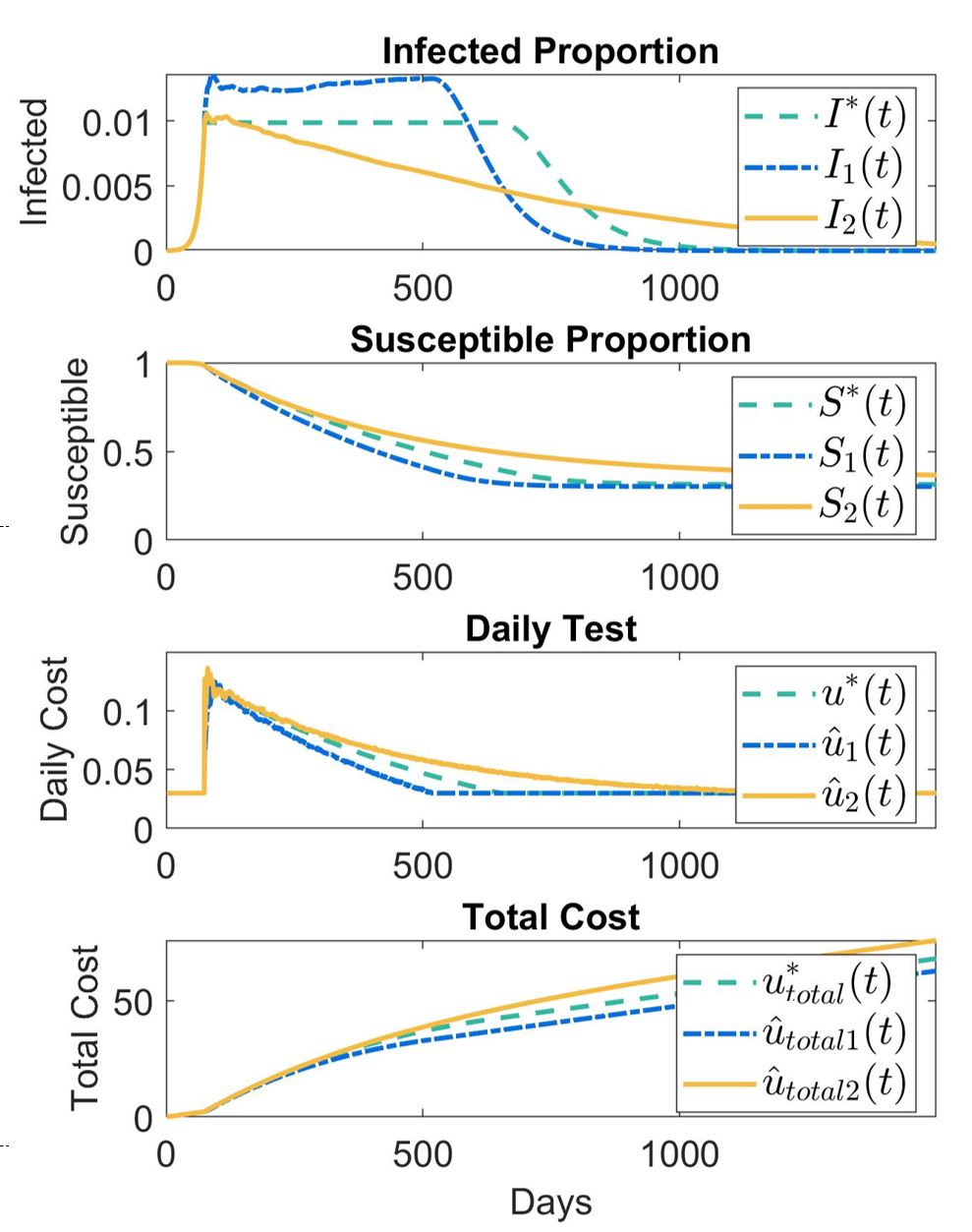

We compare the trajectories in Fig. 3. The simulation illustrates that the control system is nearly feasible by leveraging Strategy 2, as demonstrated by in Fig. 3. However, when leveraging the learned parameters directly (Strategy 1), the system becomes infeasible. As shown in Fig. 3, the infection state is still increasing after reaching . The cause of this phenomenon is that when the system starts to change the testing policy from to at the time step when , the highly underestimated transmission rate , shown in Fig. 4, leads to the underestimation of the seriousness of the epidemic, and the testing rate . Further, as illustrated in Fig. 3, during the epidemic outbreak, which will generate insufficient testing resources to maintain the infection level under the infection threshold . Recall from Lemma 3, the optimal control policy is the pointwise smallest testing strategy we can leverage to ensure the system is feasible. Hence, during the outbreak will lead to the system becoming infeasible. Regarding the second statement of Remark 1, the simulation shows that it takes longer for the system under Strategy 2 to reach the herd immunity, compared to the system under the optimal testing strategy. The daily testing generated through Strategy 2 is higher than the optimal daily testing, captured by . By comparing the simulated susceptible states, we see Strategy 2 generates fewer or equal total uninfected population at any given time step, i.e., , which implies that Strategy 2 will cause fewer people to be infected over the course of the outbreak, that is, for all .
V Conclusion
In this work, we study the impact of uncertainties introduced by parameter learning and state estimation in real-time optimal epidemic mitigation. We show the effectiveness of the proposed testing strategy when overestimating the seriousness of the epidemic under the condition that the ranges of the parameters and states are known. Compared to the optimal testing strategy, the proposed strategy can flatten the curve effectively with more cost in terms of testing and time. However, we have shown analytically that the proposed strategy generates fewer or equal cumulative infected individuals at any given time step up to the optimal herd immunity point and it appears, via simulations, to be true for all time. In the current work, we assume the ranges of both the states and parameters are known. Future work will propose strategies to learn the parameters and embed the parameter learning techniques into the proposed testing and isolation framework.
References
- [1] C. Tsay, F. Lejarza, M. A. Stadtherr, and M. Baldea, “Modeling, state estimation, and optimal control for the US COVID-19 outbreak,” Scientific Reports, vol. 10, no. 1, pp. 1–12, 2020.
- [2] T. A. Perkins and G. España, “Optimal control of the COVID-19 pandemic with non-pharmaceutical interventions,” Bulletin of Mathematical Biology, vol. 82, no. 9, pp. 1–24, 2020.
- [3] D. Acemoglu, A. Fallah, A. Giometto, D. Huttenlocher, A. Ozdaglar, F. Parise, and S. Pattathil, “Optimal adaptive testing for epidemic control: Combining molecular and serology tests,” arXiv preprint arXiv:2101.00773, 2021.
- [4] D. H. Morris, F. W. Rossine, J. B. Plotkin, and S. A. Levin, “Optimal, near-optimal, and robust epidemic control,” Communications Physics, vol. 4, no. 1, pp. 1–8, 2021.
- [5] J. Köhler, L. Schwenkel, A. Koch, J. Berberich, P. Pauli, and F. Allgöwer, “Robust and optimal predictive control of the COVID-19 outbreak,” Annual Reviews in Control, 2020.
- [6] R. Carli, G. Cavone, N. Epicoco, P. Scarabaggio, and M. Dotoli, “Model predictive control to mitigate the COVID-19 outbreak in a multi-region scenario,” Annual Reviews in Control, vol. 50, pp. 373–393, 2020.
- [7] L. Zino and M. Cao, “Analysis, prediction, and control of epidemics: A survey from scalar to dynamic network models,” IEEE Circuits and Systems Magazine, vol. 21, no. 4, pp. 4–23, 2021.
- [8] B. She, S. Sundaram, and P. E. Paré, “A learning-based model predictive control framework for real-time SIR epidemic mitigation,” in Proceedings of the American Control Conference (ACC 2022), 2022, pp. 2565 –2570.
- [9] H. Khadilkar, T. Ganu, and D. P. Seetharam, “Optimising lockdown policies for epidemic control using reinforcement learning,” Transactions of the Indian National Academy of Engineering, vol. 5, no. 2, pp. 129–132, 2020.
- [10] P. Scarabaggio, R. Carli, G. Cavone, N. Epicoco, and M. Dotoli, “Nonpharmaceutical stochastic optimal control strategies to mitigate the COVID-19 spread,” IEEE Transactions on Automation Science and Engineering, 2021.
- [11] H. Bastani, K. Drakopoulos, V. Gupta, I. Vlachogiannis, C. Hadjicristodoulou, P. Lagiou, G. Magiorkinis, D. Paraskevis, and S. Tsiodras, “Efficient and targeted COVID-19 border testing via reinforcement learning,” Nature, vol. 599, no. 7883, pp. 108–113, 2021.
- [12] M. Bloem, T. Alpcan, and T. Başar, “Optimal and robust epidemic response for multiple networks,” Control Engineering Practice, vol. 17, no. 5, pp. 525–533, 2009.
- [13] C. Nowzari, V. M. Preciado, and G. J. Pappas, “Analysis and control of epidemics: A survey of spreading processes on complex networks,” IEEE Control Systems Magazine, vol. 36, no. 1, pp. 26–46, 2016.
- [14] P. Di Giamberardino and D. Iacoviello, “Optimal control of SIR epidemic model with state dependent switching cost index,” Biomedical Signal Processing and Control, vol. 31, pp. 377–380, 2017.
- [15] O. Sharomi and T. Malik, “Optimal control in epidemiology,” Annals of Operations Research, vol. 251, no. 1-2, pp. 55–71, 2017.
- [16] P. Di Giamberardino and D. Iacoviello, “Optimal resource allocation to reduce an epidemic spread and its complication,” Information, vol. 10, no. 6, p. 213, 2019.
- [17] J. Liu, P. E. Paré, A. Nedić, C. Y. Tang, C. L. Beck, and T. Başar, “Analysis and control of a continuous-time bi-virus model,” IEEE Transactions on Automatic Control, vol. 64, no. 12, pp. 4891–4906, 2019.
- [18] C. E. Dangerfield, M. Vyska, and C. A. Gilligan, “Resource allocation for epidemic control across multiple sub-populations,” Bulletin of Mathematical Biology, vol. 81, no. 6, pp. 1731–1759, 2019.
- [19] V. M. Preciado, M. Zargham, C. Enyioha, A. Jadbabaie, and G. Pappas, “Optimal resource allocation for network protection: A geometric programming approach,” IEEE Transactions on Control of Network Systems, vol. 1, no. 1, pp. 99–108, 2014.
- [20] S. Han, V. M. Preciado, C. Nowzari, and G. J. Pappas, “Data-driven network resource allocation for controlling spreading processes,” IEEE Transactions on Network Science and Engineering, vol. 2, no. 4, pp. 127–138, 2015.
- [21] G. Chowell, “Fitting dynamic models to epidemic outbreaks with quantified uncertainty: A primer for parameter uncertainty, identifiability, and forecasts,” Infectious Disease Modelling, vol. 2, no. 3, pp. 379–398, 2017.
- [22] R. E. Baker, J.-M. Pena, J. Jayamohan, and A. Jérusalem, “Mechanistic models versus machine learning, a fight worth fighting for the biological community?” Biology Letters, vol. 14, no. 5, p. 20170660, 2018.
- [23] C. O. Wilke and C. T. Bergstrom, “Predicting an epidemic trajectory is difficult,” Proceedings of the National Academy of Sciences, vol. 117, no. 46, pp. 28 549–28 551, 2020.
- [24] F. Casella, “Can the COVID-19 epidemic be controlled on the basis of daily test reports?” IEEE Control System Letters, vol. 5, no. 3, pp. 1079–1084, 2020.
- [25] S. M. Grundel, S. Heyder, T. Hotz, T. K. S. Ritschel, P. Sauerteig, and K. Worthmann, “How to coordinate vaccination and social distancing to mitigate SARS-CoV-2 outbreaks,” SIAM Journal on Applied Dynamical Systems, vol. 20, no. 2, pp. 1135–1157, 2021.
- [26] IDA+A, “Ongoing COVID-19 results for testing administered by the Protect Purdue Health Center,” 2020, https://protect.purdue.edu/dashboard/.
- [27] W. O. Kermack and A. G. McKendrick, “A contribution to the mathematical theory of epidemics,” Proceedings of the Royal Society A, vol. 115, no. 772, pp. 700–721, 1927.
- [28] N. R. Draper and H. Smith, Applied Regression Analysis. John Wiley & Sons, 1998, vol. 326.