跳到论文正文
W Papers独立论文阅读器 arXiv:2209.01453 论文正文 计算阅读时间 · 0%
引用这篇论文根据当前论文元数据生成,正式投稿前建议核对。


License: CC BY-NC-ND 4.0
arXiv:2209.01453v1 [econ.TH] 03 Sep 2022

Learning by Consuming: Optimal Pricing with Endogenous Information ProvisionThanks: We are grateful for helpful discussions with Tilman Börgers, Ilwoo Hwang, Silvana Krasteva, R. Vijay Krishna, Rohit Lamba, Jingfeng Lu, Sergei Severinov, Vasiliki Skreta, Roland Strausz, Siyang Xiong, Jidong Zhou, as well as audiences at TAMU, UC Riverside, Wuhan University, Sun Yat-sen University, 2022 Decentralization Conference, 2022 North American Summer Meeting of the Econometric Society, 2022 Conference on Mechanism and Institution Design, and 21st SAET conference. He and Liu acknowledge financial support from the Research Grants Council of Hong Kong (14503318) and the National Natural Science Foundation of China (72192805 and 72073115), respectively.

Huiyi Guo Thanks: Huiyi Guo: Department of Economics, Texas A&M University, 4228 TAMU, College Station, TX 77843, United States of America. Email: huiyiguo@tamu.edu.    Wei He Thanks: Wei He: Department of Economics, The Chinese University of Hong Kong, Hong Kong, China. Email: hewei@cuhk.edu.hk.    Bin Liu Thanks: Bin Liu: School of Management and Economics and Shenzhen Finance Institute, The Chinese University of Hong Kong, Shenzhen (CUHK-Shenzhen), China 518172. Email: binliu@cuhk.edu.cn.
August 11, 2026
Abstract

We study the revenue-maximizing mechanism when a buyer’s value evolves endogenously because of learning-by-consuming. A seller sells one unit of a divisible good, while the buyer relies on his private, rough valuation to choose his first-stage consumption level. Consuming more leads to a more precise valuation estimate, after which the buyer determines the second-stage consumption level. The optimum is a menu of try-and-decide contracts, consisting of a first-stage price-quantity pair and a second-stage per-unit price for the remaining quantity. In equilibrium, a higher first-stage valuation buyer pays more for higher first-stage consumption and enjoys a lower second-stage per-unit price. Methodologically, we deal with the difficulty that due to the failure of single-crossing condition, monotonicity in allocation plus the envelope condition is insufficient for incentive compatibility. Our results help to understand contracts about sequential consumption with the learning feature; e.g., leasing contracts for experience goods and trial sessions for certain courses.

JEL Classification Numbers: D44, D82, D86

Keywords: Adverse selection, Dynamic mechanism design, Endogenous type distribution, Information provision, Rotation order, Experience good.

1 Introduction

Situations are abundant in which a consumer is uncertain about how well the good’s characteristics fit him at the outset, but by consuming (a portion of) the good, he could learn additional information to refine the value estimation. With such a more precise value estimate, the consumer then decides how many further units of the good to consume. Such kind of learning by consuming is widely observed in practice.

For example, car dealers in the U.S. usually provide a menu of contracts to potential consumers. Some consumers may choose to enter leasing contracts, which give them both the right to drive the car during the lease term and a lease-end option to buy out the car. The cost of the leasing contract and the buyout price depend on the length of the lease term, which usually ranges from two to four years. These consumers can learn their matching values with the car in the lease term, before deciding whether to buy out the car or not. Consumers who are more uncertain are often more willing to learn matching values by entering the leasing contracts. Other consumers may choose to buy the car outright instead. This usually happens when a consumer is sufficiently optimistic about the matching value, and hence wishes to secure a lower payment for the long-term ownership of the car.

As another example, when purchasing certain courses with fixed terms --- a one-month package of fitness classes from a gym, a two-month playgroup for pre-school toddlers, or a summer sports course for children --- the consumer often prefers to experience a few sessions first. After paying a fee and attending a few included sessions which can be viewed as trial sessions, the consumer refines his valuation and decides whether to register for additional (or the remaining) sessions or not. As in the car-leasing example, in practice, the seller often sets a price for the included sessions and another price for additional sessions, and typically both prices depend on the number/length of included sessions. It is commonly observed that the seller offers different pricing packages to the consumer, who then decides which package to choose.11 1 For example, Orangetheory Fitness, a popular fitness chain with more than a million members in the U.S., offers three monthly membership packages for consumers. These options differ with each other mainly in terms of the number of included sessions and fee structures.

There are two important features in the examples above. First, the seller can choose to first sell a portion of the good to the consumer, through which the consumer better understands how well the good fits him and then decides the subsequent consumption. Second, since the consumer’s learning is achieved through consuming, there is a tension between information acquisition and future consumption. Naturally, consuming more in the beginning would lead to a more precise value estimate, so that he could make a better decision in the future. However, at the same time, it also means that the size of the remaining portion of the good decreases. For instance, while entering a contract with a long lease term induces sufficient learning, it may make the buy-out option unattractive as the car will be getting old; experiencing more trial sessions helps the consumer better learn the valuation but decreases the number of sessions that can be sold beyond the trial.

How should the seller incorporate such kind of learning by consuming into her selling mechanism? To address this question, we study a two-stage model, in which a risk-neutral seller sells one unit of a divisible good to a risk-neutral buyer. The buyer’s valuation depends on how well the good fits him, which is uncertain to him at stage one. Yet, at stage one, he has a prior -- rough private valuation of the good. Relying on this rough valuation, he decides how many units to experience. Experiencing the good provides him with additional private information regarding the good’s characteristics. Consuming more leads to more precise additional information.22 2 The precision of the additional information through consumption is defined in the sense of rotation order, see Section 2 for details. With the updated private valuation, the buyer further determines his second-stage consumption level.

In our problem, the first-stage allocation (i.e., consumption)33 3 We use “allocation” and “consumption” interchangeably. plays two roles. First, it is the device for information acquisition, since it provides the buyer with additional information, which will be more precise with a higher first-stage allocation. Meanwhile, it also defines an intertemporal problem: It “secures” some consumption in the early period, regardless of whether the newly acquired information is good or bad, and also determines the maximum amount of consumption in the later stage. Clearly, a revenue-maximizing seller should incorporate both roles of the first-stage allocation into her pricing strategy.

We fully characterize the revenue-maximizing mechanism and find that the optimum can be implemented by a menu of try-and-decide contracts, consisting of a first-stage price-quantity pair and a second-stage per-unit price for the remaining quantity. When the buyer selects some try-and-decide contract, he needs to pay the corresponding first-stage price specified by the contract chosen. By doing this, the buyer not only gets to experience the corresponding first-stage portion (i.e., quantity) of the good, but also obtains the option to buy the remaining portion at the prescribed second-stage per-unit price. In the optimal contract, a larger first-stage consumption level (quantity) is paired with a higher first-stage price but a lower per-unit second-stage price for the remaining portion of the good. Moreover, if the buyer ends up buying the entire good across two stages, a higher first-stage consumption leads to a lower total payment. In equilibrium, a higher first-stage valuation buyer pays more to consume more in the first stage, in exchange for a lower per-unit price for the remaining portion.

The intuition is as follows. For a high first-stage valuation buyer, he is more confident that his updated valuation of the good is sufficiently high, so that he will likely buy the entire portion of the good. Thus, he is willing to pay to consume more in the first stage to enjoy a lower price for the additional consumption in the second stage, and also a lower total price for the entire portion of the good. However, this is quite risky for a low first-stage valuation buyer. If he does so, despite the second-stage per-unit price being lower, he has to pay to consume more in the first stage to enjoy this second-stage benefit. Yet, since his first-stage valuation is low, he really wants to experience the good just a bit to improve his decision in the second stage, rather than “blindly” having a high first-stage consumption level, which can lead to a low expected payoff given the low first-stage valuation.

The format of our optimal try-and-decide contracts resembles practical contracts. For instance, in the car-leasing example, the leasing price can be viewed as the first-stage price, while the length of the lease term and the buyout price can be regarded as the first-stage quantity and second-stage price. In the other course registration example, the trial sessions and the remaining sessions can be viewed as the consumption at the two stages, respectively. In this sense, we provide a rationale for the common phenomena of sequential consumption with learning in reality.

On the technical side, we would like to point out that when solving the optimal mechanism, establishing the global incentive compatibility (IC) condition is quite involved in our setting. In canonical sequential screening problems, e.g., Courty and Li 2000 and Eső and Szentes 2007a, building on local IC, the monotonicity of an allocation rule leads to global IC, even if it may not be the optimal allocation rule. By imposing certain regularity conditions, one can check that the optimal allocation rule in the relaxed problem, which only uses local IC, is indeed monotone. As a result, such an allocation rule also satisfies global IC, so that it is indeed the optimum. However, this standard approach does not apply in our setting. In fact, we provide an example where the first-stage allocation rule is monotone, but this allocation rule cannot be part of a global IC mechanism. To establish global IC of our mechanism, we have to explicitly make use of the optimality of the first-stage allocation rule. The difficulty we encounter can be better explained by focusing on the first-stage problem, where the sequential screening problem can be understood as a corresponding static screening problem; see Krähmer and Strausz 2017 for further discussions. In the corresponding static problem, a standard condition in the literature, often called the single-crossing condition (alternatively, the constant sign condition, or the Spence--Mirrlees condition), is missing. The lack of such kind of a condition prevents us from establishing global IC only from the monotonicity of the first-stage allocation rule.44 4 Krähmer and Strausz 2017 show that the condition of first-order stochastic dominance (FOSD) in the canonical sequential screening problem is equivalent to the usual single-crossing condition in a certain static screening problem. As is well known, without the single-crossing condition, solving the optimal mechanism is generally believed to be challenging even in static screening problems; see, for example, Araujo and Moreira 2010 and Schottmüller 2015. In our setting, the standard approach fails because of the violation of the single-crossing condition. This approach may also fail when the optimal solution to the standard relaxed problem is non-monotone; see Krähmer and Strausz 2015, Battaglini and Lamba 2019, Lu and Wang 2021, and Li and Shi 2022 for the analysis of optimal mechanisms in this case.

Our paper joins the growing literature on dynamic mechanism design.55 5 This is now an extensive literature; please refer to Bergemann and Välimäki 2019 for an excellent survey. The canonical literature typically assumes that the agent has two (or more) stages of private information, where the distribution of the second-stage private information is exogenously determined by the first-stage private information. In particular, it is often assumed that a higher first-stage type corresponds to a better distribution of the second-stage type in the sense of FOSD. See, for example, Courty and Li 2000, Eső and Szentes 2007a, Krähmer and Strausz 2015; Krähmer and Strausz 2017, and more recently Li and Shi 2022, as well as Battaglini 2005 and Garrett and Pavan 2012 for infinite stages. However, in the current work, the distribution of the second-stage valuation (type) depends on the first-stage consumption, which is endogenously chosen by the buyer. Due to rotation ordering,66 6 Studies that also use this information order includes, for example, Johnson and Myatt 2006, Hoffmann and Inderst 2011, and Shi 2012. such endogenously generated second-stage information is no longer ranked in terms of FOSD, which is a feature that does not exist in many canonical papers.77 7 In Liu and Lu 2018, the second-stage type’s distribution is also endogenous (determined by moral hazard), but it is ranked by FOSD.

Within the dynamic mechanism design literature, there is a strand that involves information acquisition and provision. Among these papers, the channel of information acquisition is typically independent of the product sold by the principal. One approach to model information acquisition in the literature assumes that there is an outside source of information acquisition. For example, in Eső and Szentes 2007a; Eső and Szentes 2007b, Li and Shi 2017, and Guo et al. 2022, the channel of information provision is abstract — the principal directly controls how much information to release to the agent. In Hoffmann and Inderst 2011, the principal produces two independent goods: a product itself and an additional information provision service. It is through the consumption of the information provision service that a consumer learns more about his valuation of the product. Another approach models information acquisition as a moral hazard problem or an entry problem. For example, in Krähmer and Strausz 2011, the agent can take a hidden action to gather information; in Lu et al. 2021, the agent can incur an entry cost to fully observe the ex post value. Some studies, for example, Armstrong and Zhou 2016 and Lu and Wang 2021, model the information acquisition as searches. In this paper, the buyer’s first-stage consumption plays a dual role: The buyer not only enjoys a payoff but also acquires additional information from the first-stage consumption. Such information acquisition from the allocation (i.e., consumption) itself differentiates the current work from the above-mentioned papers.

This paper also features an intertemporal problem: The first-stage allocation not only endogenously shapes the distribution of the second-stage valuation but also changes the feasibility constraint of the second-stage allocation. Pavan et al. 2014 accommodate this feature before the current work, but they focus on providing a general approach to tackle dynamic mechanism design problems. On the other hand, we explicitly characterize the optimum in a consumer-learning environment.

The rest of the paper is organized as follows. Section 2 sets up the model. We analyze the solution of a relaxed problem in Section 3 and the optimal mechanism in Section 4. Sections 5 and 6 discuss the results and conclude. The appendix collects some technical proofs.

2 The Model

A risk-neutral monopolist sells one unit of a divisible good to a risk-neutral buyer in two stages. The buyer’s true valuation VV of the good depends on how well the good fits him. At stage one, the buyer is uncertain about VV, but he observes a “rough” valuation of the good, v1v_{1}. Relying on this rough valuation, the buyer purchases q1∈[0,1]q_{1}\in[0,1] units of the good. The true valuation VV is jointly determined by v1v_{1} and the additional information v~2\tilde{v}_{2}, which is independent of v1v_{1}.88 8 The assumption that v1v_{1} and v~2\tilde{v}_{2} are independent means that the ex ante information asymmetry does not depend on the precision of the second-stage information, which helps us provide a clean characterization of the optimal mechanism. On the other hand, when considering the more general setting that v1v_{1} and v~2\tilde{v}_{2} are correlated, one has to impose additional restrictions on the information structure; see, for example, Courty and Li 2000 and Eső and Szentes 2007a. We focus on the current setting, as working with the more general structure will make the analysis much more complicated and the new insights less transparent. We assume that E⁡[v~2]=0E[\tilde{v}_{2}]=0 and V=v1+v~2V=v_{1}+\tilde{v}_{2}.99 9 Such an additive form is not an assumption, because one can define the difference between the true valuation and the rough valuation as the additional information. Consuming/experiencing q1q_{1} units of the good provides the buyer with additional information to learn about v~2\tilde{v}_{2}. With a more precise assessment of the good, at stage two, the buyer decides how many further units q2∈[0,1−q1]q_{2}\in[0,1-q_{1}] to buy. The buyer’s outside option is normalized to be 00.

From the seller’s perspective, v1v_{1} is a random draw from a cumulative distribution function (CDF) G⁡(⋅)G(\cdot), which admits a strictly positive continuous density function gg over the support [0,1][0,1].1010 10 It is without loss to assume that the support is [0,1][0,1]. The buyer learns additional information about v~2\tilde{v}_{2} through consumption: After buying q1q_{1} units of the good, the buyer forms a posterior estimate v2v_{2} of v~2\tilde{v}_{2}. From an ex ante perspective, v2v_{2} follows the CDF F(⋅|q1)F(\cdot|q_{1}). The realization of v2v_{2} is again the buyer’s private information. The seller’s goal is to design a contract that maximizes her revenue.

Intuitively, consuming more at stage one helps the buyer acquire more precise information at stage two. The precision of the additional information v2v_{2} through consumption is captured by the rotation order (Johnson and Myatt 2006; Hoffmann and Inderst 2011, cf.). Specifically, for any q1∈(0,1]q_{1}\in(0,1] and v2∈(−∞,+∞)v_{2}\in(-\infty,+\infty), F⁡(v2|q1)F(v_{2}|q_{1}) is continuously differentiable in q1q_{1} such that

∂F⁡(v2|q1)∂q1​{>0, when ​v2<0;=0, when ​v2=0;<0, when ​v2>0.\frac{\partial F(v_{2}|q_{1})}{\partial q_{1}}\begin{cases}>0,&\text{ when }v_{2}<0;\\ =0,&\text{ when }v_{2}=0;\\ <0,&\text{ when }v_{2}>0.\end{cases}

When q1=0q_{1}=0, F(⋅|q1)F(\cdot|q_{1}) degenerates to a mass at E⁡[v~2]=0E[\tilde{v}_{2}]=0, capturing no additional information gained if there is no consumption. For convenience, suppose that when q1>0q_{1}>0, F⁡(v2|q1)F(v_{2}|q_{1}) is twice continuously differentiable in v2v_{2} and the corresponding density function f⁡(v2|q1)>0f(v_{2}|q_{1})>0. We also assume that for any v2≠0v_{2}\neq 0, limq1→0+​F​(v2|q1)=F⁡(v2|0)\underset{q_{1}\rightarrow 0+}{\lim}F(v_{2}|q_{1})=F(v_{2}|0).

To illustrate the setting, consider the following “truth-or-noise” example, which has been widely used in the literature; see, for example, Lewis and Sappington 1994 and Johnson and Myatt 2006.

Example 1 (Truth-or-noise).

After consuming q1q_{1} units, the buyer observes a signal ss of v~2\tilde{v}_{2}. The signal is true (i.e., s=v~2s=\tilde{v}_{2}) with probability q1q_{1}, and is completely noisy (i.e., ss is an independent random draw from the same CDF as v~2\tilde{v}_{2}) with probability 1−q11-q_{1}. Denote the CDF of v~2\tilde{v}_{2} by H⁡(⋅)H(\cdot), which is twice continuously differentiable over the support (−∞,+∞)(-\infty,+\infty). Then, when observing the signal ss, the buyer’s posterior estimate of v~2\tilde{v}_{2} is

v2=E[v~2|s,q1]=q1s+(1−q1)E[v~2]=q1s.v_{2}=E[\tilde{v}_{2}|s,q_{1}]=q_{1}s+(1-q_{1})E[\tilde{v}_{2}]=q_{1}s.

Thus, ex ante, v2v_{2} follows the CDF F⁡(v2|q1)=H⁡(v2q1)F(v_{2}|q_{1})=H(\frac{v_{2}}{q_{1}}), which satisfies all the assumptions mentioned above.

After consuming q1q_{1} units, imagine that the buyer adopts a simple threshold plan v2v_{2}. That is, he will buy the rest 1−q11-q_{1} units at stage two only when the additional information acquired is sufficiently good — i.e., when the additional information is higher than the threshold v2v_{2}. Thus, the buyer’s expected consumption in the second stage is (1−q1)​(1−F⁡(v2|q1))(1-q_{1})(1-F(v_{2}|q_{1})), and the expected total consumption across two stages is

C⁡(v2,q1)=q1+(1−q1)​(1−F⁡(v2|q1))=1−(1−q1)​F​(v2|q1).C(v_{2},q_{1})=q_{1}+(1-q_{1})(1-F(v_{2}|q_{1}))=1-(1-q_{1})F(v_{2}|q_{1}). (1)

When q1>0q_{1}>0, it is clear that a higher threshold v2v_{2} — i.e., requiring better information — leads to a drop in CC, as the partial derivative with respect to v2v_{2},

∂C⁡(v2,q1)∂v2=−(1−q1)​f​(v2|q1)<0.\frac{\partial C(v_{2},q_{1})}{\partial v_{2}}=-(1-q_{1})f(v_{2}|q_{1})<0.

However, the effect of a higher first-stage consumption q1q_{1} on CC is ambiguous. The “marginal rate of substitution” is

M⁡(v2,q1)=∂C⁡(v2,q1)∂q1∂C⁡(v2,q1)∂v2=−11−q1​F⁡(v2|q1)f⁡(v2|q1)+∂F⁡(v2|q1)∂q1f⁡(v2|q1)M(v_{2},q_{1})=\frac{\frac{\partial C(v_{2},q_{1})}{\partial q_{1}}}{\frac{\partial C(v_{2},q_{1})}{\partial v_{2}}}=-\frac{1}{1-q_{1}}\frac{F(v_{2}|q_{1})}{f(v_{2}|q_{1})}+\frac{\frac{\partial F(v_{2}|q_{1})}{\partial q_{1}}}{f(v_{2}|q_{1})}

for any (v2,q1)∈ℝ×(0,1)(v_{2},q_{1})\in\mathbb{R}\times(0,1).

We make the following assumption regarding M⁡(v2,q1)M(v_{2},q_{1}).

Assumption 1.

For any fixed q1∈(0,1)q_{1}\in(0,1) and v2<v2′v_{2}<v_{2}^{\prime},

M⁡(v2,q1)≤0⟹M⁡(v2′,q1)<0.M(v_{2},q_{1})\leq 0\quad\Longrightarrow\quad M(v_{2}^{\prime},q_{1})<0.
Remark 1.

Assumption 1 is a natural assumption regarding the substitution between the first-stage consumption and the additional information. It says that: If at a particular level of first-stage consumption q1q_{1} and a certain requirement of additional information v2v_{2}, the buyer is willing to sacrifice his first-stage consumption in exchange for a lower requirement of information (i.e., a lower v2v_{2}), then he will still be willing to do so when the requirement of information is more stringent than v2v_{2} (i.e., higher than v2v_{2}).

Note that Assumption 1 holds when F⁡(v2|q1)/f⁡(v2|q1)F(v_{2}|q_{1})/f(v_{2}|q_{1}) is increasing in v2v_{2} and ∂F⁡(v2|q1)∂q1/f⁡(v2|q1)\frac{\partial F(v_{2}|q_{1})}{\partial q_{1}}/f(v_{2}|q_{1}) is decreasing in v2v_{2}. The former condition is a standard hazard rate assumption. The latter one is the same as Assumption 3 in Shi 2012, which can be interpreted as supermodularity. In the truth-or-noise example above, the latter assumption is automatically satisfied, while the former assumption is satisfied when H⁡(x)/h⁡(x)H(x)/h(x) is increasing in xx.

Finally, we make the following standard hazard rate assumption about GG.

Assumption 2.

We assume that 1−G⁡(v1)g⁡(v1)\frac{1-G(v_{1})}{g(v_{1})} is strictly decreasing in v1v_{1}.

We shall focus on truthful direct mechanisms {q1​(r1),q2​(r1,r2),t⁡(r1,r2)}r1∈[0,1],r2∈ℝ\{q_{1}(r_{1}),q_{2}(r_{1},r_{2}),t(r_{1},r_{2})\}_{r_{1}\in[0,1],r_{2}\in\mathbb{R}}, which is without loss of generality; see Myerson 1986. In the first stage, when the buyer reports r1r_{1}, the seller allocates q1​(r1)q_{1}(r_{1}) units of the good to him. In the second stage, v2v_{2} is realized according to F(⋅|q1(r1))F(\cdot|q_{1}(r_{1})). Given the buyer’s second-stage report r2r_{2}, the seller allocates q2​(r1,r2)q_{2}(r_{1},r_{2}) units of the good to the buyer and demands a payment t⁡(r1,r2)t(r_{1},r_{2}).

2.1 The buyer’s problem

Suppose that the buyer truthfully reported v1v_{1} at stage one, but he reports r2r_{2} despite that the true second-stage type is v2v_{2}. Let π~​(v1,r2,v2)\tilde{\pi}(v_{1},r_{2},v_{2}) be his expected payoff at stage two:

π~​(v1,r2,v2)=(v1+v2)​q2​(v1,r2)−t⁡(v1,r2).\tilde{\pi}(v_{1},r_{2},v_{2})=(v_{1}+v_{2})q_{2}(v_{1},r_{2})-t(v_{1},r_{2}).

Envelope theorem yields

d⁡π~​(v1,v2,v2)d⁡v2=∂π~​(v1,r2,v2)∂v2|r2=v2=q2​(v1,v2).\frac{\rmd\tilde{\pi}(v_{1},v_{2},v_{2})}{\rmd v_{2}}=\frac{\partial\tilde{\pi}(v_{1},r_{2},v_{2})}{\partial v_{2}}|_{r_{2}=v_{2}}=q_{2}(v_{1},v_{2}).

Denote ψ⁡(v1)=v1−1−G⁡(v1)g⁡(v1)\psi(v_{1})=v_{1}-\frac{1-G(v_{1})}{g(v_{1})}, which is strictly increasing by Assumption 2. The following result is standard (Eső and Szentes 2007a, see, e.g.,), and its proof is omitted.

Lemma 1.
  1. (i)

    Suppose that the buyer reports the first-stage type v1v_{1} truthfully. The second-stage IC constraint is satisfied if and only if the following two conditions hold:

    1. (a)

      For any v1v_{1} and v2v_{2},1111 11 When v2<−ψ⁡(v1)v_{2}<-\psi(v_{1}), ∫−ψ⁡(v1)v2q2(v1,s)ds=−∫v2−ψ⁡(v1)q2(v1,s)ds\int_{-\psi(v_{1})}^{v_{2}}q_{2}(v_{1},s)\rmd s=-\int_{v_{2}}^{-\psi(v_{1})}q_{2}(v_{1},s)\rmd s.

      π~​(v1,v2,v2)=π~​(v1,−ψ⁡(v1),−ψ⁡(v1))+∫−ψ⁡(v1)v2q2​(v1,s)​d⁡s.\tilde{\pi}(v_{1},v_{2},v_{2})=\tilde{\pi}(v_{1},-\psi(v_{1}),-\psi(v_{1}))+\int_{-\psi(v_{1})}^{v_{2}}q_{2}(v_{1},s)\rmd s. (2)
    2. (b)

      The second-stage allocation q2​(v1,v2)q_{2}(v_{1},v_{2}) is increasing in v2v_{2} for any v1v_{1}.

  2. (ii)

    On the other hand, suppose that the buyer’s first-stage type is v1v_{1} but he reported r1r_{1} in the first stage. Then, when he observes v2v_{2} in the second stage, he will report r2=r2​(v1,r1,v2)r_{2}=r_{2}(v_{1},r_{1},v_{2}) such that

    r1+r2​(v1,r1,v2)=v1+v2.r_{1}+r_{2}(v_{1},r_{1},v_{2})=v_{1}+v_{2}.

Based on Lemma 1, the expected payoff of the buyer with first-stage type v1v_{1} and report r1r_{1} can be expressed as

U⁡(v1,r1)\displaystyle U(v_{1},r_{1}) =\displaystyle= q1​(r1)​∫−∞+∞(v1+v2)​F​(d⁡v2|q1​(r1))\displaystyle q_{1}(r_{1})\int_{-\infty}^{+\infty}(v_{1}+v_{2})F(\rmd v_{2}|q_{1}(r_{1}))
+∫−∞+∞[(v1+v2)​q2​(r1,r2​(v1,r1,v2))−t⁡(r1,r2​(v1,r1,v2))]F(dv2|q1(r1)).\displaystyle+\int_{-\infty}^{+\infty}\left[\begin{array}[]{c}(v_{1}+v_{2})q_{2}(r_{1},r_{2}(v_{1},r_{1},v_{2}))\\ -t(r_{1},r_{2}(v_{1},r_{1},v_{2}))\end{array}\right]F(\rmd v_{2}|q_{1}(r_{1})).

The first-stage IC constraint requires that for any v1v_{1} and r1r_{1},

U⁡(v1,v1)≥U⁡(v1,r1).U(v_{1},v_{1})\geq U(v_{1},r_{1}).

The following result provides a necessary condition for the first-stage IC constraint (all the proofs are relegated to the Appendix).

Lemma 2.

The first-stage IC constraint implies that for any v1v_{1}

U⁡(v1,v1)=U⁡(0,0)+∫0v1[q1​(s)+∫−∞+∞q2​(s,v2)​F​(d⁡v2|q1​(s))]​d⁡s.U(v_{1},v_{1})=U(0,0)+\int_{0}^{v_{1}}\left[q_{1}(s)+\int_{-\infty}^{+\infty}q_{2}(s,v_{2})F(\rmd v_{2}|q_{1}(s))\right]\rmd s.

2.2 The seller’s problem

The seller’s expected revenue is the difference between the social welfare and the buyer’s ex ante expected payoff. By Lemma 2, it can be written as

R\displaystyle R =\displaystyle= ∫01{v1​q1​(v1)+∫−∞+∞(v1+v2)​q2​(v1,v2)​F​(d⁡v2|q1​(v1))}​g​(v1)​d⁡v1\displaystyle\int_{0}^{1}\left\{v_{1}q_{1}(v_{1})+\int_{-\infty}^{+\infty}(v_{1}+v_{2})q_{2}(v_{1},v_{2})F(\rmd v_{2}|q_{1}(v_{1}))\right\}g(v_{1})\rmd v_{1}
−∫01U(v1,v1)g(v1)dv1\displaystyle-\int_{0}^{1}U(v_{1},v_{1})g(v_{1})\rmd v_{1}
=\displaystyle= ∫01[ψ⁡(v1)​q1​(v1)+∫−∞+∞[ψ(v1)+v2]q2(v1,v2)F(dv2|q1(v1))]​g​(v1)​d⁡v1−U⁡(0,0).\displaystyle\int_{0}^{1}\left[\begin{array}[]{c}\psi(v_{1})q_{1}(v_{1})\\ +\int_{-\infty}^{+\infty}[\psi(v_{1})+v_{2}]q_{2}(v_{1},v_{2})F(\rmd v_{2}|q_{1}(v_{1}))\end{array}\right]g(v_{1})\rmd v_{1}-U(0,0).

Now we are ready to state the seller’s problem as follows.

Problem (O):max(q1,q2,t)R\mbox{Problem (O)}:\qquad\max_{(q_{1},q_{2},t)}R\qquad\qquad\qquad\qquad\qquad

subject to

constraint (2) and q2(v1,v2) is increasing in v2 for any v1;\text{constraint (\ref{e2'}) and }q_{2}(v_{1},v_{2})\text{ is increasing in }v_{2}\text{ for any }v_{1}; (5)
U⁡(v1,v1)≥U⁡(v1,r1)​, for any ​v1,r1;U(v_{1},v_{1})\geq U(v_{1},r_{1})\text{, for any }v_{1},r_{1}; (6)
0≤q1​(v1)≤1​ and ​0≤q2​(v1,v2)≤1−q1​(v1)​, for any ​v1,v2.0\leq q_{1}(v_{1})\leq 1\text{ and }0\leq q_{2}(v_{1},v_{2})\leq 1-q_{1}(v_{1})\text{, for any }v_{1},v_{2}. (7)

Here, (5) is the equivalent condition for the second-stage IC constraint, (6) is the first-stage IC constraint, and (7) is the feasibility constraint imposed on allocations.

Clearly, at the optimum, U⁡(0,0)=0U(0,0)=0, and thus the seller’s ex ante revenue becomes

R=∫01[ψ⁡(v1)​q1​(v1)+∫−∞+∞[ψ(v1)+v2]q2(v1,v2)F(dv2|q1(v1))]​g​(v1)​d⁡v1.R=\int_{0}^{1}\left[\begin{array}[]{c}\psi(v_{1})q_{1}(v_{1})\\ +\int_{-\infty}^{+\infty}[\psi(v_{1})+v_{2}]q_{2}(v_{1},v_{2})F(\rmd v_{2}|q_{1}(v_{1}))\end{array}\right]g(v_{1})\rmd v_{1}.

We further drop constraints (5) to (6) and omit the choice variable tt to form a relaxed problem, Problem (O-R):

max(q1,q2)⁡R\max_{(q_{1},q_{2})}R
 subject to constraint (7).\mbox{ subject to constraint (\ref{fesibility})}.

If the solution to Problem (O-R) also satisfies (5) and (6), then such a solution also solves Problem (O). As such, we will first solve Problem (O-R), and then verify that its solution satisfies all the constraints in the original problem.

3 The solution to Problem (O-R)

In Problem (O-R), for each fixed first-stage allocation rule q1q_{1}, the following second-stage allocation rule q2q_{2} obviously maximizes the objective function RR:

q2​(v1,v2)={1−q1​(v1), if ​ψ​(v1)+v2≥0;0, otherwise.q_{2}(v_{1},v_{2})=\begin{cases}1-q_{1}(v_{1}),&\text{ if }\psi(v_{1})+v_{2}\geq 0;\\ 0,&\text{ otherwise.}\end{cases}

Thus, we have1212 12 The detailed derivation can be found in the Appendix.

R\displaystyle R =\displaystyle= ∫01[ψ⁡(v1)​q1​(v1)+∫−ψ⁡(v1)+∞[ψ⁡(v1)+v2]​(1−q1​(v1))​F​(d⁡v2|q1​(v1))]​g​(v1)​d⁡v1\displaystyle\int_{0}^{1}\left[\psi(v_{1})q_{1}(v_{1})+\int_{-\psi(v_{1})}^{+\infty}[\psi(v_{1})+v_{2}](1-q_{1}(v_{1}))F(\rmd v_{2}|q_{1}(v_{1}))\right]g(v_{1})\rmd v_{1} (8)
=\displaystyle= ∫01[ψ⁡(v1)+(1−q1​(v1))​∫−∞−ψ⁡(v1)F⁡(v2|q1​(v1))​d​v2]​g​(v1)​d​v1.\displaystyle\int_{0}^{1}\left[\psi(v_{1})+(1-q_{1}(v_{1}))\int_{-\infty}^{-\psi(v_{1})}F(v_{2}|q_{1}(v_{1}))\rmd v_{2}\right]g(v_{1})\rmd v_{1}.

To facilitate the presentation, define the seller’s revenue from a type-v1v_{1} buyer with the first-stage consumption q1q_{1} as

Π⁡(q1,v1)=ψ⁡(v1)+(1−q1)​∫−∞−ψ⁡(v1)F⁡(v2|q1)​d⁡v2.\Pi(q_{1},v_{1})=\psi(v_{1})+(1-q_{1})\int_{-\infty}^{-\psi(v_{1})}F(v_{2}|q_{1})\rmd v_{2}. (9)

For each v1v_{1}, let q1∗​(v1)q_{1}^{\ast}(v_{1}) be the maximizer of Π⁡(q1,v1)\Pi(q_{1},v_{1}) in q1∈[0,1]q_{1}\in[0,1]. Finally, define

v1∗=ψ−1​(0)​ and ​v~1=inf{v1∈[0,1]:q1∗​(v1)>0}.v_{1}^{\ast}=\psi^{-1}(0)\text{ and }\tilde{v}_{1}=\inf\{v_{1}\in[0,1]:q_{1}^{\ast}(v_{1})>0\}.

We have the following observation.

Lemma 3.

The following allocation rule pair {q1∗​(v1),q2∗​(v1,v2)}v1∈[0,1],v2∈ℝ\{q^{*}_{1}(v_{1}),q^{*}_{2}(v_{1},v_{2})\}_{v_{1}\in[0,1],v_{2}\in\mathbb{R}} solves Problem (O-R):

  1. (i)

    The first-stage allocation q1∗​(v1)q_{1}^{\ast}(v_{1}) is the maximizer of

    Π⁡(q1,v1)=ψ⁡(v1)+(1−q1)​∫−∞−ψ⁡(v1)F⁡(v2|q1)​d⁡v2\Pi(q_{1},v_{1})=\psi(v_{1})+(1-q_{1})\int_{-\infty}^{-\psi(v_{1})}F(v_{2}|q_{1})\rmd v_{2}

    in q1∈[0,1]q_{1}\in[0,1] for each v1v_{1}. In particular, there exists a cutoff v~1<v1∗\tilde{v}_{1}<v_{1}^{\ast} such that for all v1∈[0,v~1)v_{1}\in[0,\tilde{v}_{1}), q1∗​(v1)=0q_{1}^{\ast}(v_{1})=0. For all v1∈[v~1,1]v_{1}\in[\tilde{v}_{1},1], q1∗​(v1)∈[0,1)q_{1}^{\ast}(v_{1})\in[0,1) and can be characterized by the first-order condition:

    ∫−∞−ψ⁡(v1)[−F⁡(v2|q1∗​(v1))+(1−q1∗​(v1))​∂F⁡(v2|q1∗​(v1))∂q1]​d⁡v2=0.\int_{-\infty}^{-\psi(v_{1})}\left[-F(v_{2}|q_{1}^{\ast}(v_{1}))+(1-q_{1}^{\ast}(v_{1}))\frac{\partial F(v_{2}|q_{1}^{\ast}(v_{1}))}{\partial q_{1}}\right]\rmd v_{2}=0. (10)

    Moreover, for all v1∈(v~1,1]v_{1}\in(\tilde{v}_{1},1], q1∗​(v1)∈(0,1)q^{*}_{1}(v_{1})\in(0,1).

  2. (ii)

    The second-stage allocation rule q2∗q^{*}_{2} is

    q2∗​(v1,v2)={1−q1∗​(v1), if ​ψ​(v1)+v2≥0;0, otherwise.q^{*}_{2}(v_{1},v_{2})=\begin{cases}1-q^{*}_{1}(v_{1}),&\text{ if }\psi(v_{1})+v_{2}\geq 0;\\ 0,&\text{ otherwise.}\end{cases}

    In particular, when v1<v~1v_{1}<\tilde{v}_{1}, F(⋅|q1∗(v1))F(\cdot|q^{*}_{1}(v_{1})) degenerates to a mass at 00 and q2∗​(v1,0)=0q^{*}_{2}(v_{1},0)=0.

The above lemma implies that there is a first-stage cutoff type v~1\tilde{v}_{1}, below which both the first-stage allocation and the second-stage allocation are zero. Hence, there is no consumption at the bottom of the distribution GG. Moreover, this cutoff is strictly below v1∗v_{1}^{\ast}. This is because a low first-stage value v1v_{1} buyer would still be willing to experience the good a bit in the first stage, as he knows that his ex post value (i.e., v1+v2v_{1}+v_{2}) is still likely to be high enough. The seller then should take advantage of this by setting a positive allocation for such low first-stage types. However, when the first-stage type is so low (below v~1\tilde{v}_{1}) that the ex post value is quite unlikely to be sufficiently high, the buyer does not find it worthwhile to experience the good; so the seller, anticipating this, should set a zero first-stage allocation in this case.

The following result characterizes the monotonicity of the optimal first-stage allocation rule.

Lemma 4.

The first-stage allocation q1∗​(v1)q_{1}^{\ast}(v_{1}) is strictly increasing in v1∈[v~1,1]v_{1}\in[\tilde{v}_{1},1].

Remark 2.

It is worth pointing out that Π⁡(q1,v1)\Pi(q_{1},v_{1}) does not have the supermodularity or single-crossing property in (q1,v1)(q_{1},v_{1}). As a result, the standard approach of monotone comparative statics (Milgrom and Shannon 1994, e.g.,) is not readily applicable in our setting.

Remark 3.

To ease the notations and presentation, we do not take into account the possibility that for some v1v_{1}, the maximizer q1∗​(v1)q_{1}^{\ast}(v_{1}) may not be unique. This multiplicity issue can be addressed by imposing the following assumption analogous to Assumption 1:

  • •

    For any fixed v2≤0v_{2}\leq 0 and any q1,q1′∈(0,1)q_{1},q_{1}^{\prime}\in(0,1) with q1<q1′q_{1}<q_{1}^{\prime},

    M⁡(v2,q1)≤0⟹M⁡(v2,q1′)<0.M(v_{2},q_{1})\leq 0\qquad\Longrightarrow\qquad M(v_{2},q_{1}^{\prime})<0.

This assumption can be interpreted as a natural substitution condition, which says that: If at a particular level of first-stage consumption q1q_{1} and a certain requirement of additional information v2v_{2}, the buyer is willing to sacrifice his first-stage consumption in exchange for a lower requirement of information, then he will still be willing to do so when his first-stage consumption is higher than q1q_{1}. Under this condition, one can show that any selection of maximizers must be strictly increasing in v1v_{1} when v1≥v~1v_{1}\geq\tilde{v}_{1}. The proof of this claim is given in the Appendix.

4 The solution to Problem (O)

4.1 Optimal direct mechanism

Having characterized the solution to Problem (O-R) as in Lemma 3, we can use the envelope conditions in Lemmas 1 and 2 to construct a payment rule t∗t^{*}, the expression of which is provided in the following result.

Lemma 5.

The payment rule t∗t^{\ast} is specified as follows:

t∗​(v1,v2)={(1−q1∗​(v1))​p2∗​(v1)+p1∗​(v1), if ​ψ​(v1)+v2≥0,p1∗​(v1), otherwise,t^{\ast}(v_{1},v_{2})=\begin{cases}(1-q_{1}^{\ast}(v_{1}))p^{*}_{2}(v_{1})+p_{1}^{\ast}(v_{1}),&\mbox{ if }\psi(v_{1})+v_{2}\geq 0,\\ p_{1}^{\ast}(v_{1}),&\text{ otherwise},\end{cases}

where

p1∗​(v1)\displaystyle p_{1}^{\ast}(v_{1}) =(1−q1∗​(v1))​[∫−∞−ψ⁡(v1)F⁡(v2|q1∗​(v1))​d⁡v2−1−G⁡(v1)g⁡(v1)]\displaystyle=(1-q_{1}^{\ast}(v_{1}))\bigg[\int_{-\infty}^{-\psi(v_{1})}F(v_{2}|q_{1}^{\ast}(v_{1}))\rmd v_{2}-\frac{1-G(v_{1})}{g(v_{1})}\bigg]
+∫0v1(1−q1∗(x))F(−ψ(x)|q1∗(x))dx\displaystyle\quad+\int_{0}^{v_{1}}(1-q_{1}^{\ast}(x))F(-\psi(x)|q_{1}^{\ast}(x))\rmd x

and

p2∗​(v1)=1−G⁡(v1)g⁡(v1).p_{2}^{\ast}(v_{1})=\frac{1-G(v_{1})}{g(v_{1})}.

Thus, we obtain a candidate mechanism {q1∗​(v1),q2∗​(v1,v2),t∗​(v1,v2)}v1∈[0,1],v2∈ℝ\{q_{1}^{\ast}(v_{1}),q_{2}^{\ast}(v_{1},v_{2}),t^{\ast}(v_{1},v_{2})\}_{v_{1}\in[0,1],v_{2}\in\mathbb{R}} for Problem (O). If we can show that this candidate mechanism satisfies all constraints in Problem (O), then it must solve Problem (O). Clearly, one only needs to verify constraints (5) and (6) — i.e., the first- and second-stage IC constraints.

To this end, we begin by considering a menu of try-and-decide option contracts {p1∗​(v1),q1∗​(v1);p2∗​(v1)}v1∈[0,1]\{p^{*}_{1}(v_{1}),q^{*}_{1}(v_{1});p^{*}_{2}(v_{1})\}_{v_{1}\in[0,1]}, where functions p1∗p^{*}_{1}, q1∗q^{*}_{1}, and p2∗p^{*}_{2} are defined in Lemmas 3 and 5. The buyer needs to select a contract from the menu. If for some r1∈[0,1]r_{1}\in[0,1], option contract {p1∗​(r1),q1∗​(r1);p2∗​(r1)}\{p^{*}_{1}(r_{1}),q^{*}_{1}(r_{1});p^{*}_{2}(r_{1})\} is selected, then p1∗​(r1)p^{*}_{1}(r_{1}) is the advance payment for a buyer to enter this contract. By paying this advance payment, the buyer not only consumes q1∗​(r1)q^{*}_{1}(r_{1}) units of the good, but also reserves the right to buy the remaining 1−q1∗​(r1)1-q^{*}_{1}(r_{1}) units at the per-unit strike price p2∗​(r1)p^{*}_{2}(r_{1}).

In the Appendix, we show that this menu of contracts implements the above-mentioned direct mechanism. Hence, our direct mechanism satisfies constraints (5) and (6), and thus is a solution to Problem (O), which is the following result.

Proposition 1.

The direct mechanism {q1∗​(v1),q2∗​(v1,v2),t∗​(v1,v2)}v1∈[0,1],v2∈ℝ\{q_{1}^{\ast}(v_{1}),q_{2}^{\ast}(v_{1},v_{2}),t^{\ast}(v_{1},v_{2})\}_{v_{1}\in[0,1],v_{2}\in\mathbb{R}} can be implemented by a menu of try-and-decide option contracts {p1∗​(v1),q1∗​(v1);p2∗​(v1)}v1∈[0,1]\{p_{1}^{\ast}(v_{1}),q_{1}^{\ast}(v_{1});p_{2}^{\ast}(v_{1})\}_{v_{1}\in[0,1]}. Hence, this direct mechanism solves Problem (O).

What is crucial in the proof of the above proposition is to establish global IC. The argument to establish IC in our problem is non-standard. In many canonical sequential screening problems in the literature, e.g., Courty and Li 2000 and Eső and Szentes 2007a, as long as the allocation rule satisfies certain monotonicity condition in private types, regardless of whether it is the solution of the relaxed problem or not, the allocation rule can be used to construct a direct mechanism satisfying global IC. However, this approach does not work for our problem. Intuitively, the complication arises because the first-stage allocation plays a dual role in our problem — a higher first-stage consumption is associated with a higher precision of information, but reduces the potential second-stage consumption. We sketch the key step of our argument in Section 4.2 and discuss further in Section 5.

4.2 Sketch of the proof

To establish Proposition 1, the two global IC constraints in Problem (O) require that: Facing the menu of contracts {p1∗​(v1),q1∗​(v1);p2∗​(v1)}v1∈[0,1]\{p_{1}^{\ast}(v_{1}),q_{1}^{\ast}(v_{1});p_{2}^{\ast}(v_{1})\}_{v_{1}\in[0,1]}, for each v1∈[0,1]v_{1}\in[0,1], (i) a type-v1v_{1} buyer who is under contract {p1∗​(v1),q1∗​(v1);p2∗​(v1)}\{p_{1}^{\ast}(v_{1}),q_{1}^{\ast}(v_{1});p_{2}^{\ast}(v_{1})\} will buy the remaining 1−q1∗​(v1)1-q_{1}^{\ast}(v_{1}) units if and only if v1+v2≥p2∗​(v1)v_{1}+v_{2}\geq p_{2}^{\ast}(v_{1}), and (ii) for any r1∈[0,1]r_{1}\in[0,1], a type-v1v_{1} buyer has no strict incentive to choose contract {p1∗​(r1),q1∗​(r1);p2∗​(r1)}\{p_{1}^{\ast}(r_{1}),q_{1}^{\ast}(r_{1});p_{2}^{\ast}(r_{1})\} over {p1∗​(v1),q1∗​(v1);p2∗​(v1)}\{p_{1}^{\ast}(v_{1}),q_{1}^{\ast}(v_{1});p_{2}^{\ast}(v_{1})\}, regardless of his second-stage strategy after choosing {p1∗​(r1),q1∗​(r1);p2∗​(r1)}\{p_{1}^{\ast}(r_{1}),q_{1}^{\ast}(r_{1});p_{2}^{\ast}(r_{1})\}. Parts (i) and (ii) correspond to the second- and first-stage IC constraints of the direct mechanism, respectively. It is easy to see that (i) is trivial. Hence, we focus on (ii).

Under contract {p1∗​(r1),q1∗​(r1);p2∗​(r1)}\{p_{1}^{\ast}(r_{1}),q_{1}^{\ast}(r_{1});p_{2}^{\ast}(r_{1})\}, the optimal second-stage strategy for a type-v1v_{1} buyer who learns v2v_{2} is to buy the remaining portion if and only if v2≥p2∗​(r1)−v1v_{2}\geq p^{*}_{2}(r_{1})-v_{1}. Under the above contract and the optimal second-stage strategy, the type-v1v_{1} buyer’s interim payoff is U⁡(v1,r1)=w⁡(q1∗​(r1),p2∗​(r1),v1)−p1∗​(r1)U(v_{1},r_{1})=w(q^{*}_{1}(r_{1}),p^{*}_{2}(r_{1}),v_{1})-p^{*}_{1}(r_{1}), where for all q1∈[0,1]q_{1}\in[0,1], p2≥0p_{2}\geq 0, and v1∈[0,1]v_{1}\in[0,1],

w⁡(q1,p2,v1)≡q1​v1+∫p2−v1+∞(v1+v2−p2)​(1−q1)​F​(d⁡v2|q1).w(q_{1},p_{2},v_{1})\equiv q_{1}v_{1}+\int_{p_{2}-v_{1}}^{+\infty}(v_{1}+v_{2}-p_{2})(1-q_{1})F(\rmd v_{2}|q_{1}).

It is shown in the Appendix that the difference of interim payoffs between selecting {p1∗​(v1),q1∗​(v1);p2∗​(v1)}\{p^{*}_{1}(v_{1}),q^{*}_{1}(v_{1});p^{*}_{2}(v_{1})\} and {p1∗​(r1),q1∗​(r1);p2∗​(r1)}\{p^{*}_{1}(r_{1}),q^{*}_{1}(r_{1});p^{*}_{2}(r_{1})\}, Δ⁡(v1,r1)=U⁡(v1,v1)−U⁡(v1,r1)\Delta(v_{1},r_{1})=U(v_{1},v_{1})-U(v_{1},r_{1}), is1313 13 In this paper, w3w_{3} means partial derivative with respect to the third variable; likewise, w31w_{31} means the second-order partial derivative with respect to the first and the third variables. Other partial derivatives’ notations are analogous.

∫r1v1∫xv1[w31​(q1∗​(x),p2∗​(x),s)​q1∗′​(x)+w32​(q1∗​(x),p2∗​(x),s)​p2∗′​(x)]​d⁡s​d⁡x.\displaystyle\int^{v_{1}}_{r_{1}}\int^{v_{1}}_{x}\left[\begin{array}[]{c}w_{31}(q^{*}_{1}(x),p^{*}_{2}(x),s){q_{1}^{*}}^{\prime}(x)+w_{32}(q^{*}_{1}(x),p^{*}_{2}(x),s){p_{2}^{*}}^{\prime}(x)\end{array}\right]\rmd s\rmd x.

Clearly, the first-stage IC constraint holds if and only if Δ⁡(v1,r1)≥0\Delta(v_{1},r_{1})\geq 0. To this end, it can be easily shown that w32​(q1,p2,v1)≤0w_{32}(q_{1},p_{2},v_{1})\leq 0 for all q1∈[0,1]q_{1}\in[0,1], p2≥0p_{2}\geq 0, and v1∈[0,1]v_{1}\in[0,1]. We have established in Lemma 5 that p2∗​(v1)=1−G⁡(v1)g⁡(v1)p^{*}_{2}(v_{1})=\frac{1-G(v_{1})}{g(v_{1})} and thus p2∗′​(⋅)<0{p_{2}^{*}}^{\prime}(\cdot)<0 by Assumption 2. Hence, the second term in the integrand of the double integral (4.2), w32​(q1∗​(x),p2∗​(x),s)​p2∗′​(x)≥0w_{32}(q^{*}_{1}(x),p^{*}_{2}(x),s){p_{2}^{*}}^{\prime}(x)\geq 0. Therefore, it suffices to show that the first term in the integrand is nonnegative.

By Lemmas 3 and 4, q1∗′​(⋅)≥0{q_{1}^{*}}^{\prime}(\cdot)\geq 0. However, the sign of

w31​(q1,p2,v1)=F⁡(p2−v1|q1)−(1−q1)​∂F⁡(p2−v1|q1)∂q1w_{31}(q_{1},p_{2},v_{1})=F(p_{2}-v_{1}|q_{1})-(1-q_{1})\frac{\partial F(p_{2}-v_{1}|q_{1})}{\partial q_{1}}

is ambiguous. To see this, notice that due to rotation order, when p2>v1p_{2}>v_{1}, w31>0w_{31}>0; but when p2<v1p_{2}<v_{1}, w31w_{31} can be positive or negative. The ambiguity of the sign of w31w_{31} implies that the sign of w31​(q1∗​(x),p2∗​(x),s)​q1∗′​(x)w_{31}(q^{*}_{1}(x),p^{*}_{2}(x),s){q_{1}^{*}}^{\prime}(x) is ambiguous in general when ss is between xx and v1v_{1} in (4.2). Putting these observations together, the sign of the integrand in double integral (4.2) is ambiguous.

We remark that our analysis so far has only used the observation that q1∗′​(⋅)≥0{q_{1}^{*}}^{\prime}(\cdot)\geq 0. Hence, the ambiguity of the sign of the integrand is not only an issue of our optimal q1∗​(⋅)q_{1}^{*}(\cdot), but also a problem for more general first-stage allocation rules.

After some transformation, we will obtain that

∫r1v1∫xv1w31​(q1∗​(x),p2∗​(x),s)​q1∗′​(x)​d​s​d​x=∫r1v1q1∗′​(x)​∫−ψ⁡(x)x−v1−ψ⁡(x)ξ⁡(y,q1∗​(x))​d​y​d​x,\int^{v_{1}}_{r_{1}}\int^{v_{1}}_{x}w_{31}(q^{*}_{1}(x),p^{*}_{2}(x),s){q_{1}^{*}}^{\prime}(x)\rmd s\rmd x=\int^{v_{1}}_{r_{1}}{q_{1}^{*}}^{\prime}(x)\int^{x-v_{1}-\psi(x)}_{-\psi(x)}\xi(y,q^{*}_{1}(x))\rmd y\rmd x, (12)

where ξ⁡(y,q1∗​(x))≡−∂C⁡(y,q1∗​(x))∂q1∗​(x)\xi(y,q^{*}_{1}(x))\equiv-\frac{\partial C(y,q^{*}_{1}(x))}{\partial q^{*}_{1}(x)}.1414 14 Recall that the function C⁡(⋅,⋅)C(\cdot,\cdot) is defined in (1). By the optimality of q1∗​(⋅)q^{*}_{1}(\cdot) (i.e., the first-order condition (10) which implies that ∫−∞−ψ⁡(x)ξ⁡(y,q1∗​(x))​d⁡y=0\int_{-\infty}^{-\psi(x)}\xi(y,q^{*}_{1}(x))\rmd y=0) as well as Assumption 1, we can show that for v1≥r1v_{1}\geq r_{1} (resp. v1≤r1v_{1}\leq r_{1}),

∫−ψ⁡(x)x−v1−ψ⁡(x)ξ⁡(y,q1∗​(x))​d⁡y≥0\int^{x-v_{1}-\psi(x)}_{-\psi(x)}\xi(y,q^{*}_{1}(x))\rmd y\geq 0

(resp. ≤0\leq 0) for xx between v1v_{1} and r1r_{1}. Hence, the double integral (12) is nonnegative. It is trivial that

∫r1v1∫xv1w32​(q1∗​(x),p2∗​(x),s)​p2∗′​(x)​d⁡s​d⁡x≥0.\int^{v_{1}}_{r_{1}}\int^{v_{1}}_{x}w_{32}(q^{*}_{1}(x),p^{*}_{2}(x),s){p_{2}^{*}}^{\prime}(x)\rmd s\rmd x\geq 0.

Combining the two inequalities above, one can conclude that Δ⁡(v1,r1)≥0\Delta(v_{1},r_{1})\geq 0.

4.3 Implementation

The following lemma summarizes several useful properties of the payment rule, and we will discuss them after Proposition 2.

Lemma 6.
  1. (i)

    For v1<v~1v_{1}<\tilde{v}_{1}, p1∗​(v1)=0p_{1}^{\ast}(v_{1})=0 and t∗​(v1,0)=0t^{*}(v_{1},0)=0.

  2. (ii)

    The first-stage payment p1∗​(v1)p_{1}^{\ast}(v_{1}) is strictly increasing in v1∈[v~1,1]v_{1}\in[\tilde{v}_{1},1] and equal to q1∗​(v~1)​1−G⁡(v~1)g⁡(v~1)≥0q^{*}_{1}(\tilde{v}_{1})\frac{1-G(\tilde{v}_{1})}{g(\tilde{v}_{1})}\geq 0 for v1=v~1v_{1}=\tilde{v}_{1}.

  3. (iii)

    The second-stage payment p2∗​(v1)p_{2}^{\ast}(v_{1}) is strictly decreasing in v1∈[0,1]v_{1}\in[0,1] and equal to zero when v1=1v_{1}=1.

  4. (iv)

    The function p1∗​(v1)+(1−q1∗​(v1))​p2∗​(v1)p_{1}^{\ast}(v_{1})+(1-q_{1}^{\ast}(v_{1}))p_{2}^{\ast}(v_{1}) is strictly decreasing in v1∈[0,1]v_{1}\in[0,1].

  5. (v)

    The function p1∗​(v1)+(1−q1∗​(v1))​p2∗​(v1)​(1−F⁡(−ψ⁡(v1)|q1∗​(v1)))p_{1}^{\ast}(v_{1})+(1-q_{1}^{\ast}(v_{1}))p_{2}^{\ast}(v_{1})(1-F(-\psi(v_{1})|q^{*}_{1}(v_{1}))) is strictly increasing in v1∈[v~1,1]v_{1}\in[\tilde{v}_{1},1] and equal to zero elsewhere.

Remark 4 (No participation at the bottom).

According to Lemmas 3 and 6 (i), when v1<v~1v_{1}<\tilde{v}_{1}, there is zero consumption in both stages and the total payment is zero. As such, the buyer with the first-stage type lower than v~1\tilde{v}_{1} is completely shut down — he does not participate.

According to Remark 4, it is immediate that the “reduced” menu of try-and-decide option contracts {p1∗​(v1),q1∗​(v1);p2∗​(v1)}v1∈[v~1,1]\{p_{1}^{\ast}(v_{1}),q_{1}^{\ast}(v_{1});p_{2}^{\ast}(v_{1})\}_{v_{1}\in[\tilde{v}_{1},1]} implements the solution of Problem (O), since a buyer with first-stage type v1<v~1v_{1}<\tilde{v}_{1} simply does not participate. Hence, we have the following result.

Proposition 2.

The solution of Problem (O) can be implemented by a menu of try-and-decide option contracts {p1∗​(v1),q1∗​(v1);p2∗​(v1)}v1∈[v~1,1]\{p_{1}^{\ast}(v_{1}),q_{1}^{\ast}(v_{1});p_{2}^{\ast}(v_{1})\}_{v_{1}\in[\tilde{v}_{1},1]}.

According to Lemmas 4 and 6, the first-stage payment p1∗​(v1)p_{1}^{\ast}(v_{1}) and consumption q1∗​(v1)q_{1}^{\ast}(v_{1}) are strictly increasing when v1≥v~1v_{1}\geq\tilde{v}_{1}. However, the per-unit strike price p2∗​(v1)p_{2}^{\ast}(v_{1}) is strictly decreasing, and the total payment conditional on buying the entire portion of the good — i.e., p1∗​(v1)+(1−q1∗​(v1))​p2∗​(v1)p_{1}^{\ast}(v_{1})+(1-q^{*}_{1}(v_{1}))p_{2}^{\ast}(v_{1}) — is strictly decreasing in v1v_{1}. This implies that in equilibrium, a buyer with a higher first-stage type will choose a contract with a higher advance payment and higher first-stage consumption, in exchange for a lower per-unit strike price for additional consumption in the second stage and a lower cost for purchasing the entire unit of the good.

The intuition is clear. For a high v1v_{1}-type buyer, he is more confident that his ex post valuation of the good, v1+v2v_{1}+v_{2}, is sufficiently high so that he will likely end up buying the entire good. The buyer is thus incentivized to choose a contract that “secures” a large first-stage consumption and first-stage payment so that he can enjoy a lower per-unit strike price in stage two and a lower cost for purchasing the entire unit. However, this will be quite risky for a low v1v_{1}-type. If he does so, in spite of a lower per-unit second-stage price, he has to pay to consume more in the first stage. Yet, since his first-stage type is low, he really wants to experience the good a bit to make a better decision in the second stage, rather than “blindly” having a high first-stage consumption level, which can lead to a rather low expected payoff given his low first-stage type.

This intuition echoes phenomena seen in practice. For example, consumers who are optimistic about their matching quality with a car tend to buy the car outright, because buying the car outright is usually cheaper than leasing it with the intention to buy out the car at lease end. However, those who are not as optimistic may choose to lease the car first before making a buyout decision. This practice can be expensive, but gives consumers an opportunity to experience the car before committing to it for a longer duration.

Lemma 6 (v) implies that Π⁡(q1∗​(v1),v1)\Pi(q^{*}_{1}(v_{1}),v_{1}) is strictly increasing in v1v_{1} for v1∈[v~1,1]v_{1}\in[\tilde{v}_{1},1]. Namely, the seller can expect to extract more surplus from a higher first-stage type.

4.4 An illustrative example

In this section, we provide an illustrative example, which demonstrates the optimal mechanism that is identified in Proposition 1. In addition, we shall also illustrate that the monotonicity of the first-stage allocation rule does not imply global IC. To be precise, we explicitly construct an increasing first-stage allocation rule q^1\hat{q}_{1}, and show that it cannot be part of an incentive-compatible mechanism.

Recall the truth-or-noise model in Example 1. Let GG be the uniform distribution on [0,1][0,1] with the constant density g≡1g\equiv 1, and HH be the normal distribution N⁡(0,1)N(0,1) with mean 00 and variance 11 (i.e., the density is h⁡(v2)=12​π​e−v222h(v_{2})=\frac{1}{\sqrt{2\pi}}e^{-\frac{v_{2}^{2}}{2}}). Then ψ⁡(v1)=2​v1−1\psi(v_{1})=2v_{1}-1,

F⁡(v2|q1)=H⁡(v2q1)=∫−∞v2q112​π​e−s22​d⁡s, and f⁡(v2|q1)=1q1​2​π​e−v222​q12.F(v_{2}|q_{1})=H(\frac{v_{2}}{q_{1}})=\int_{-\infty}^{\frac{v_{2}}{q_{1}}}\frac{1}{\sqrt{2\pi}}e^{-\frac{s^{2}}{2}}\rmd s,\quad\mbox{ and }\quad f(v_{2}|q_{1})=\frac{1}{q_{1}\sqrt{2\pi}}e^{-\frac{v_{2}^{2}}{2q^{2}_{1}}}.

In the Appendix, we verify that FF satisfies the rotation order, and Assumptions 1 and 2 hold.

As shown in Proposition 1, the optimal first-stage allocation rule q1∗q_{1}^{*} must maximize

(1−q1)​∫−∞−ψ⁡(v1)F⁡(v2|q1)​d⁡v2.(1-q_{1})\int_{-\infty}^{-\psi(v_{1})}F(v_{2}|q_{1})\rmd v_{2}.

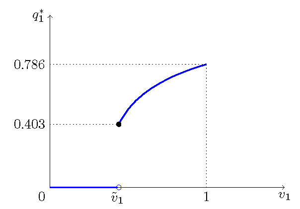
Figure 2 numerically illustrates the optimal allocation rule.1515 15 In this example, we plot the figures by simulation. In this example, v~1≈0.43<0.5=v1∗\tilde{v}_{1}\approx 0.43<0.5=v_{1}^{*}. In Figure 2, we plot Π⁡(q1,v1)\Pi(q_{1},v_{1}) when v1=0.41v_{1}=0.41, 0.430.43, and 0.450.45. As can be seen, q1∗​(v1)q_{1}^{*}(v_{1}) is unique and higher than q1∗​(v~1)≈0.403q_{1}^{*}(\tilde{v}_{1})\approx 0.403 when v1>v~1≈0.43v_{1}>\tilde{v}_{1}\approx 0.43, is either 00 or almost 0.4030.403 when v1=v~1v_{1}=\tilde{v}_{1}, and is 00 when v1<v~1v_{1}<\tilde{v}_{1}. This pattern explains the jump of q1∗q_{1}^{*} at v~1\tilde{v}_{1} in Figure 2.

Refer to caption
Figure 1: q1∗q_{1}^{*}
Figure 2: Π⁡(q1,v1)\Pi(q_{1},v_{1})

Below, we construct another allocation rule (q^1CLOSE(\hat{q}_{1}, OPENq^2)\hat{q}_{2}):

q^1​(v1)={ψ2​(v1),v1≥12,0,otherwise;q^2​(v1,v2)={1−q^1​(v1),ψ⁡(v1)+v2≥0,0, otherwise.\hat{q}_{1}(v_{1})=\begin{cases}\psi^{2}(v_{1}),&v_{1}\geq\frac{1}{2},\\ 0,&\mbox{otherwise};\end{cases}\qquad\hat{q}_{2}(v_{1},v_{2})=\begin{cases}1-\hat{q}_{1}(v_{1}),&\psi(v_{1})+v_{2}\geq 0,\\ 0,&\mbox{ otherwise}.\end{cases}

It is clear that q^1\hat{q}_{1} is increasing. In the Appendix, we show that (q^1CLOSE(\hat{q}_{1}, OPENq^2)\hat{q}_{2}) cannot be the allocation rule in an incentive-compatible mechanism.

5 Discussions

5.1 Monotonicity does not imply global IC

In many canonical sequential screening problems in the literature (Courty and Li 2000; Eső and Szentes 2007a, cf.), as long as the allocation rule satisfies certain monotonicity condition, regardless of whether it is the solution of the relaxed problem, the allocation rule can be used to construct a mechanism satisfying global IC. As such, the standard treatment in the literature focuses on identifying sufficient conditions under which the solution of the relaxed problem is monotone. However, this approach does not work in the current paper and we will discuss our approach by connecting it with the literature.

By nicely linking a canonical sequential screening problem to a static screening problem, Krähmer and Strausz 2017 show that the first-order stochastic dominance (FOSD) ranking of first-stage types in a canonical sequential screening problem as in Courty and Li 2000 corresponds to the single-crossing condition1616 16 The single-crossing condition is also refereed to as the Spence-Mirrlees condition or the constant sign condition in the literature. Note that this condition should not be confused with the one required by our Assumption 1. To minimize confusion, we use the term single-crossing condition to refer to the standard condition imposed by canonical screening problems exclusively. in the corresponding static screening problem; and conversely, a sequential screening problem without FOSD corresponds to a static screening problem without the single-crossing condition. With FOSD, the above-mentioned standard treatment in sequential screening problems — i.e., finding sufficient conditions under which the optimal allocation rule in a certain relaxed problem is monotone — works for establishing global IC. This is similar to the well-known result that in static screening problems, the single-crossing condition ensures that local IC plus monotonicity of the allocation rule implies global IC.

However, the counterpart of the single-crossing condition does not hold in our corresponding static screening problem, as types are not ranked by FOSD here. More specifically, in the corresponding static screening problem, the condition requires that w31w_{31} has a constant sign in the respective integration region in our optimal solution, but as we have discussed in Section 4.2, w31w_{31} does not satisfy this property.1717 17 The lack of single-crossing condition issue has been discussed by Araujo and Moreira 2010 and Schottmüller 2015 in their respective static screening environments. Due to the lack of the single-crossing condition, rather than just establishing the monotonicity of the allocation rule as in canonical sequential screening problems, we need to deal with global IC in a non-standard way; indeed, the monotonicity of allocation rule does not imply global IC, as seen in the example in Section 4.4. In particular, as is illustrated in Sections 4.2 and 4.4, the optimality of the first-stage allocation rule, i.e., the fact that the first-stage allocation rule solves the relaxed problem, is explicitly used in establishing global IC, and this contrasts with many canonical sequential screening problems.

We remark that the expression of w31w_{31} is complicated. In particular, the cutoff point at which w31w_{31} changes sign depends on v1v_{1}, p2p_{2}, and q1q_{1} simultaneously. This is due to the dual role played by the first-stage allocation. First, the first-stage allocation is a device of information acquisition. Second, it defines an intertemporal problem: It affects the feasibility constraint of the second-stage allocation, as the second-stage allocation cannot exceed the remaining portion of the good. In problems where the first-stage allocation only affects information acquisition (Hoffmann and Inderst 2011, cf.), the counterpart of w31w_{31} has a more clear-cut structure — the point at which their w31w_{31} changes sign depends on v1v_{1} and p2p_{2} only. The dual role of our first-stage allocation leads to new observations as we will discuss in Sections 5.2 and 5.3.

5.2 Monotonicity of the first-stage allocation rule

Notice that at the optimum, a higher first-stage type always consumes more, and thus he acquires more information. This is a bit counter-intuitive. After all, a sufficiently high type does not need to actively acquire additional information, because his current information (first-stage type) is already sufficiently good; similarly, a sufficiently low type also does not want to incur a cost to acquire information, because his current information is already so bad that costly information acquisition is not beneficial. Thus, intuitively, only “middle” types have a strong incentive to acquire information. In fact, this is indeed the case in the continuous information acquisition model of Hoffmann and Inderst 2011 and the discrete information acquisition model of Krähmer and Strausz 2011. In particular, Hoffmann and Inderst 2011 study a similar problem as our paper. They show that the level of information acquisition is of hump shape: The level first increases and then decreases in the first-stage type.

The crucial difference is that in our paper, the first-stage consumption plays a dual role for the buyer. On the one hand, it is a device for acquiring more information that shapes the distribution of additional information as in these papers; on the other hand, it also directly changes the buyer’s payoff by determining the division between the first- and second-stage consumption. The latter role is absent in these papers.

5.3 Distortion

Finally, we compare the consumption levels in both stages with their counterparts in the first-best scenario, in which the buyer’s first- and second-stage types are public. Denote the buyer’s first- and second-stage types as v1v_{1} and v2v_{2}, respectively. Let q1F​B​(v1)q_{1}^{FB}(v_{1}) and q2F​B​(v1,v2)q_{2}^{FB}(v_{1},v_{2}) be his socially efficient first- and second-stage consumption, respectively. The expected social surplus from a buyer with first-stage type v1v_{1} is

v1​q1F​B​(v1)+∫−∞+∞(v1+v2)​q2F​B​(v1,v2)​F​(d⁡v2|q1FB​(v1)).v_{1}q_{1}^{FB}(v_{1})+\int_{-\infty}^{+\infty}(v_{1}+v_{2})q_{2}^{FB}(v_{1},v_{2})F(\rmd v_{2}|q_{1}^{FB}(v_{1})).

Suppose q1F​Bq_{1}^{FB} is given. Then, the first-best q2F​Bq_{2}^{FB} is

q2F​B​(v1,v2)={1−q1F​B​(v1), if ​v1+v2≥0;0, otherwise.q_{2}^{FB}(v_{1},v_{2})=\begin{cases}1-q^{FB}_{1}(v_{1}),&\text{ if }v_{1}+v_{2}\geq 0;\\ 0,&\text{ otherwise.}\end{cases}

Thus, the above expression of social surplus can be written as1818 18 The derivation is almost the same as that for the integral in (8); one just needs to replace ψ⁡(v1)\psi(v_{1}) and q1​(v1)q_{1}(v_{1}) there with v1v_{1} and q1F​B​(v1)q_{1}^{FB}(v_{1}), respectively.

v1​q1F​B​(v1)+∫−v1+∞(v1+v2)​(1−q1F​B​(v1,v2))​F​(d⁡v2|q1FB​(v1))\displaystyle v_{1}q_{1}^{FB}(v_{1})+\int_{-v_{1}}^{+\infty}(v_{1}+v_{2})(1-q_{1}^{FB}(v_{1},v_{2}))F(\rmd v_{2}|q_{1}^{FB}(v_{1}))
=\displaystyle= v1+(1−q1F​B​(v1))​∫−∞−v1F⁡(v2|q1F​B​(v1))​d⁡v2.\displaystyle v_{1}+(1-q_{1}^{FB}(v_{1}))\int_{-\infty}^{-v_{1}}F(v_{2}|q_{1}^{FB}(v_{1}))\rmd v_{2}.

Therefore, q1F​B​(v1)q_{1}^{FB}(v_{1}) maximizes the function

Π~​(q1,v1)=v1+(1−q1)​∫−∞−v1F⁡(v2|q1)​d⁡v2.\tilde{\Pi}(q_{1},v_{1})=v_{1}+(1-q_{1})\int_{-\infty}^{-v_{1}}F(v_{2}|q_{1})\rmd v_{2}.

Comparing with (9), one can see that q1F​B​(ψ⁡(v1))=q1∗​(v1)q_{1}^{FB}(\psi(v_{1}))=q_{1}^{\ast}(v_{1}) for all v1∈[v1∗,1]v_{1}\in[v^{*}_{1},1]. This leads to q1F​B​(v1)=q1∗​(ψ−1​(v1))q_{1}^{FB}(v_{1})=q_{1}^{\ast}(\psi^{-1}(v_{1})) for all v1∈[0,1]v_{1}\in[0,1]. By Lemma 4, the fact that ψ\psi is strictly increasing, and the fact that ψ−1​(0)=v1∗>v~1\psi^{-1}(0)=v^{*}_{1}>\tilde{v}_{1}, q1F​Bq_{1}^{FB} is strictly increasing. Also, recall that v1≥ψ⁡(v1)v_{1}\geq\psi(v_{1}) with strict inequality when v1∈[0,1)v_{1}\in[0,1), we have q1F​B​(v1)≥q1F​B​(ψ⁡(v1))=q1∗​(v1)q_{1}^{FB}(v_{1})\geq q_{1}^{FB}(\psi(v_{1}))=q_{1}^{\ast}(v_{1}) with strict inequality when v1∈[0,1)v_{1}\in[0,1). We summarize these observations below.

Proposition 3.
  1. (i)

    q1F​B​(v1)=q1∗​(ψ−1​(v1))q_{1}^{FB}(v_{1})=q_{1}^{\ast}(\psi^{-1}(v_{1})) for all v1∈[0,1]v_{1}\in[0,1];

  2. (ii)

    q1F​B​(v1)q_{1}^{FB}(v_{1}) is strictly increasing when v1∈[0,1]v_{1}\in[0,1];

  3. (iii)

    q1F​B​(v1)≥q1∗​(v1)q_{1}^{FB}(v_{1})\geq q_{1}^{\ast}(v_{1}), with strict inequality when v1∈[0,1)v_{1}\in[0,1).

The above proposition implies that in general, there is an under-provision of information when asymmetric information arises compared to the first best. This again differs from Hoffmann and Inderst 2011 and Krähmer and Strausz 2011, in which there can be an over- and under-provision of information, depending on the first-stage type.

Now let us focus on the case that v1∈[0,1)v_{1}\in[0,1) to compare the optimal and the first-best second-stage allocations. For v2≥−ψ⁡(v1)v_{2}\geq-\psi(v_{1}), q2F​B​(v1,v2)<q2∗​(v1,v2)q^{FB}_{2}(v_{1},v_{2})<q^{*}_{2}(v_{1},v_{2}) and q1F​B​(v1)+q2F​B​(v1,v2)=q1∗​(v1)+q2∗​(v1,v2)=1q^{FB}_{1}(v_{1})+q^{FB}_{2}(v_{1},v_{2})=q^{*}_{1}(v_{1})+q^{*}_{2}(v_{1},v_{2})=1; for v2∈[−v1,−ψ(v1))v_{2}\in[-v_{1},-\psi(v_{1})), q2F​B​(v1,v2)>q2∗​(v1,v2)=0q^{FB}_{2}(v_{1},v_{2})>q^{*}_{2}(v_{1},v_{2})=0 and q1F​B​(v1)+q2F​B​(v1,v2)=1>q1∗​(v1)+q2∗​(v1,v2)q^{FB}_{1}(v_{1})+q^{FB}_{2}(v_{1},v_{2})=1>q^{*}_{1}(v_{1})+q^{*}_{2}(v_{1},v_{2}); for v2<−v1v_{2}<-v_{1}, q2F​B​(v1,v2)=q2∗​(v1,v2)=0q^{FB}_{2}(v_{1},v_{2})=q^{*}_{2}(v_{1},v_{2})=0 and q1F​B​(v1)+q2F​B​(v1,v2)>q1∗​(v1)+q2∗​(v1,v2)q^{FB}_{1}(v_{1})+q^{FB}_{2}(v_{1},v_{2})>q^{*}_{1}(v_{1})+q^{*}_{2}(v_{1},v_{2}). This means that although the second-stage consumption can be upward or downward distorted, the total consumption can only be downward distorted.

6 Concluding Remarks

In this paper, we study the two-stage revenue-maximizing mechanism when the buyer acquires additional information by first-stage consumption. The buyer’s decision of first-stage consumption depends on his private, prior valuation of the good. A higher first-stage consumption level leads to a more precise value estimate of the good but reduces the available amount of consumption left for the second stage. The key feature of our model is that the first-stage consumption plays a dual rule: The buyer not only enjoys a payoff but also acquires additional information from the first-stage consumption.

We fully characterize the optimum and find that it can be implemented by a menu of try-and-decide option contracts, consisting of a first-stage price-quantity pair and a second-stage per-unit price for the remaining quantity. A larger first-stage quantity is paired with a higher first-stage price but a lower second-stage per-unit price. In equilibrium, a higher first-stage valuation buyer pays more to have higher first-stage consumption and enjoys a lower second-stage price.

Since the second-stage type’s distribution is not ranked by first-order stochastic dominance, we face the difficulty of the failure of the single-crossing condition when establishing global IC. The monotonicity in the first-stage consumption plus local IC is not sufficient for global IC. As such, we cannot apply the usual approach as in many dynamic mechanism design papers, which assume FOSD, to establish global IC.

In our current analysis, we assumed that the second-stage type’s distribution only depends on the first-stage consumption. A more general environment is when it depends on both the first-stage consumption level and the first-stage type. This is a highly meaningful but challenging direction to explore. We leave it for future work.

References

  • Araujo and Moreira (2010) Araujo, A. and H. Moreira (2010). Adverse selection problems without the Spence–Mirrlees condition. Journal of Economic Theory 145(3), 1113–1141.
  • Armstrong and Zhou (2016) Armstrong, M. and J. Zhou (2016). Search deterrence. The Review of Economic Studies 83(1), 26–57.
  • Battaglini (2005) Battaglini, M. (2005). Long-term contracting with Markovian consumers. American Economic Review 95(3), 637–658.
  • Battaglini and Lamba (2019) Battaglini, M. and R. Lamba (2019). Optimal dynamic contracting: The first-order approach and beyond. Theoretical Economics 14(4), 1435–1482.
  • Bergemann and Välimäki (2019) Bergemann, D. and J. Välimäki (2019). Dynamic mechanism design: An introduction. Journal of Economic Literature 57(2), 235–74.
  • Courty and Li (2000) Courty, P. and H. Li (2000). Sequential screening. The Review of Economic Studies 67(4), 697–717.
  • Eső and Szentes (2007a) Eső, P. and B. Szentes (2007a). Optimal information disclosure in auctions and the handicap auction. The Review of Economic Studies 74(3), 705–731.
  • Eső and Szentes (2007b) Eső, P. and B. Szentes (2007b). The price of advice. The RAND Journal of Economics 38(4), 863–880.
  • Garrett and Pavan (2012) Garrett, D. F. and A. Pavan (2012). Managerial turnover in a changing world. Journal of Political Economy 120(5), 879–925.
  • Guo et al. (2022) Guo, Y., H. Li, and X. Shi (2022). Optimal discriminatory disclosure. Working paper.
  • Hoffmann and Inderst (2011) Hoffmann, F. and R. Inderst (2011). Pre-sale information. Journal of Economic Theory 146(6), 2333–2355.
  • Johnson and Myatt (2006) Johnson, J. P. and D. P. Myatt (2006). On the simple economics of advertising, marketing, and product design. American Economic Review 96(3), 756–784.
  • Krähmer and Strausz (2011) Krähmer, D. and R. Strausz (2011). Optimal procurement contracts with pre-project planning. The Review of Economic Studies 78(3), 1015–1041.
  • Krähmer and Strausz (2015) Krähmer, D. and R. Strausz (2015). Ex post information rents in sequential screening. Games and Economic Behavior 90, 257–273.
  • Krähmer and Strausz (2017) Krähmer, D. and R. Strausz (2017). Sequential versus static screening: An equivalence result. Games and Economic Behavior 106, 317–328.
  • Lewis and Sappington (1994) Lewis, T. R. and D. E. Sappington (1994). Supplying information to facilitate price discrimination. International Economic Review, 309–327.
  • Li and Shi (2017) Li, H. and X. Shi (2017). Discriminatory information disclosure. American Economic Review 107(11), 3363–85.
  • Li and Shi (2022) Li, H. and X. Shi (2022). Stochastic sequential screening. Working paper.
  • Liu and Lu (2018) Liu, B. and J. Lu (2018). Pairing provision price and default remedy: optimal two-stage procurement with private R&D efficiency. The RAND Journal of Economics 49(3), 619–655.
  • Lu and Wang (2021) Lu, J. and Z. Wang (2021). Optimal selling mechanisms with buyer price search. Journal of Economic Theory 196, 105307.
  • Lu et al. (2021) Lu, J., L. Ye, and X. Feng (2021). Orchestrating information acquisition. American Economic Journal: Microeconomics 13(4), 420–65.
  • Milgrom and Segal (2002) Milgrom, P. and I. Segal (2002). Envelope theorems for arbitrary choice sets. Econometrica 70(2), 583–601.
  • Milgrom and Shannon (1994) Milgrom, P. and C. Shannon (1994). Monotone comparative statics. Econometrica, 157–180.
  • Myerson (1986) Myerson, R. B. (1986). Multistage games with communication. Econometrica, 323–358.
  • Pavan et al. (2014) Pavan, A., I. Segal, and J. Toikka (2014). Dynamic mechanism design: A Myersonian approach. Econometrica 82(2), 601–653.
  • Schottmüller (2015) Schottmüller, C. (2015). Adverse selection without single crossing: Monotone solutions. Journal of Economic Theory 158, 127–164.
  • Shi (2012) Shi, X. (2012). Optimal auctions with information acquisition. Games and Economic Behavior 74(2), 666–686.

Appendix A Appendix

A.1 Proof of Lemma 2

By Lemma 1, the expected payoff of the buyer with first-stage type v1v_{1} and report r1r_{1} can be expressed as

U⁡(v1,r1)=\displaystyle U(v_{1},r_{1})= q1​(r1)​∫−∞+∞(v1+v2)​F​(d⁡v2|q1​(r1))\displaystyle q_{1}(r_{1})\int_{-\infty}^{+\infty}(v_{1}+v_{2})F(\rmd v_{2}|q_{1}(r_{1}))
+∫−∞+∞[(v1+v2)​q2​(r1,r2​(v1,r1,v2))−t⁡(r1,r2​(v1,r1,v2))]F(dv2|q1(r1)).\displaystyle+\int_{-\infty}^{+\infty}\left[\begin{array}[]{c}(v_{1}+v_{2})q_{2}(r_{1},r_{2}(v_{1},r_{1},v_{2}))\\ -t(r_{1},r_{2}(v_{1},r_{1},v_{2}))\end{array}\right]F(\rmd v_{2}|q_{1}(r_{1})).
=\displaystyle= q1​(r1)​v1+∫−∞+∞[(v1+v2)​q2​(r1,r2​(v1,r1,v2))−t⁡(r1,r2​(v1,r1,v2))]​F​(d⁡v2|q1​(r1)),\displaystyle q_{1}(r_{1})v_{1}+\int_{-\infty}^{+\infty}\left[\begin{array}[]{c}(v_{1}+v_{2})q_{2}(r_{1},r_{2}(v_{1},r_{1},v_{2}))\\ -t(r_{1},r_{2}(v_{1},r_{1},v_{2}))\end{array}\right]F(\rmd v_{2}|q_{1}(r_{1})),

where the second equality uses the fact that E⁡[v2]=0E[v_{2}]=0. Taking the partial derivative with respect to v1v_{1} leads to1919 19 The (almost everywhere) differentiability of q2q_{2} and tt in r2r_{2} follows from the second-stage IC constraint.

∂U⁡(v1,r1)∂v1=q1​(r1)+∫−∞+∞{q2​(r1,r2​(v1,r1,v2))+∂r2​(v1,r1,v2)∂v1​[(v1+v2)​∂q2​(r1,r2​(v1,r1,v2))∂r2−∂t⁡(r1,r2​(v1,r1,v2))∂r2]}​F​(d⁡v2|q1​(r1)).\frac{\partial U(v_{1},r_{1})}{\partial v_{1}}=q_{1}(r_{1})+\int_{-\infty}^{+\infty}\left\{\begin{array}[]{c}q_{2}(r_{1},r_{2}(v_{1},r_{1},v_{2}))\\ +\frac{\partial r_{2}(v_{1},r_{1},v_{2})}{\partial v_{1}}\left[\begin{array}[]{c}(v_{1}+v_{2})\frac{\partial q_{2}(r_{1},r_{2}(v_{1},r_{1},v_{2}))}{\partial r_{2}}\\ -\frac{\partial t(r_{1},r_{2}(v_{1},r_{1},v_{2}))}{\partial r_{2}}\end{array}\right]\end{array}\right\}F(\rmd v_{2}|q_{1}(r_{1})).

Sincer2​(v1,r1,v2)\ r_{2}(v_{1},r_{1},v_{2}) is the optimal report following a lie in the first stage — i.e., it maximizes the second-stage expected payoff after a lie — it must satisfy the first-order condition, so

(v1+v2)​∂q2​(r1,r2​(v1,r1,v2))∂r2−∂t⁡(r1,r2​(v1,r1,v2))∂r2=0.(v_{1}+v_{2})\frac{\partial q_{2}(r_{1},r_{2}(v_{1},r_{1},v_{2}))}{\partial r_{2}}-\frac{\partial t(r_{1},r_{2}(v_{1},r_{1},v_{2}))}{\partial r_{2}}=0.

Therefore,

∂U⁡(v1,r1)∂v1=q1​(r1)+∫−∞+∞q2​(r1,r2​(v1,r1,v2))​F​(d⁡v2|q1​(r1)).\frac{\partial U(v_{1},r_{1})}{\partial v_{1}}=q_{1}(r_{1})+\int_{-\infty}^{+\infty}q_{2}(r_{1},r_{2}(v_{1},r_{1},v_{2}))F(\rmd v_{2}|q_{1}(r_{1})).

Note that r2​(v1,r1,v2)=v2r_{2}(v_{1},r_{1},v_{2})=v_{2} when r1=v1r_{1}=v_{1} (i.e., a truthful report in the first stage). The envelope theorem (Milgrom and Segal 2002, cf.) implies that

U⁡(v1,v1)=U⁡(0,0)+∫0v1[q1​(s)+∫−∞+∞q2​(s,v2)​F​(d⁡v2|q1​(s))]​d⁡s.U(v_{1},v_{1})=U(0,0)+\int_{0}^{v_{1}}\left[q_{1}(s)+\int_{-\infty}^{+\infty}q_{2}(s,v_{2})F(\rmd v_{2}|q_{1}(s))\right]\rmd s.

This completes the proof. □\square

A.2 Derivation of Equation (8)

Before proving Equation (8), we first prove the following preparatory lemma.

Lemma 7.

For any a∈(−∞,+∞)a\in(-\infty,+\infty) and q1>0q_{1}>0,

∫−∞av2​F​(d⁡v2|q1)=aF⁡(a|q1)−∫−∞aF⁡(v2|q1)​d⁡v2.\int_{-\infty}^{a}v_{2}F(\rmd v_{2}|q_{1})=aF(a|q_{1})-\int_{-\infty}^{a}F(v_{2}|q_{1})\rmd v_{2}.
Proof.

We first claim that as b→−∞b\to-\infty, b​F​(b|q1)→0bF(b|q_{1})\to 0. Suppose that the claim is not true. Then there exists some ϵ>0\epsilon>0 and a negative sequence {bk}\{b_{k}\} that converges to −∞-\infty such that |bk|​F​(bk|q1)>ϵ|b_{k}|F(b_{k}|q_{1})>\epsilon for any kk. Since the integral ∫−∞+∞v2​F​(d⁡v2|q1)\int_{-\infty}^{+\infty}v_{2}F(\rmd v_{2}|q_{1}) is well defined, there exists some sufficiently large KK such that for any k≥Kk\geq K, ∫−∞bk|v2|​F​(d⁡v2|q1)<ϵ\int_{-\infty}^{b_{k}}|v_{2}|F(\rmd v_{2}|q_{1})<\epsilon. It implies that

|bk|​F​(bk|q1)=∫−∞bk|bk|​F​(d⁡v2|q1)≤∫−∞bk|v2|​F​(d⁡v2|q1)<ϵ,|b_{k}|F(b_{k}|q_{1})=\int_{-\infty}^{b_{k}}|b_{k}|F(\rmd v_{2}|q_{1})\leq\int_{-\infty}^{b_{k}}|v_{2}|F(\rmd v_{2}|q_{1})<\epsilon,

which is a contradiction.

For any b<min⁡{a,0}b<\min\{a,0\}, due to integral by parts,

∫bav2​F​(d⁡v2|q1)=aF⁡(a|q1)−bF⁡(b|q1)−∫baF⁡(v2|q1)​d⁡v2.\int_{b}^{a}v_{2}F(\rmd v_{2}|q_{1})=aF(a|q_{1})-bF(b|q_{1})-\int_{b}^{a}F(v_{2}|q_{1})\rmd v_{2}.

It implies that

∫baF⁡(v2|q1)​d⁡v2=aF⁡(a|q1)−bF⁡(b|q1)−∫bav2​F​(d⁡v2|q1).\int_{b}^{a}F(v_{2}|q_{1})\rmd v_{2}=aF(a|q_{1})-bF(b|q_{1})-\int_{b}^{a}v_{2}F(\rmd v_{2}|q_{1}).

It is obvious that ∫baF⁡(v2|q1)​d⁡v2\int_{b}^{a}F(v_{2}|q_{1})\rmd v_{2} is decreasing in bb. In addition, it is bounded as b​F​(b|q1)→0bF(b|q_{1})\to 0 and ∫bav2​F​(d⁡v2|q1)→∫−∞av2​F​(d⁡v2|q1)\int_{b}^{a}v_{2}F(\rmd v_{2}|q_{1})\to\int_{-\infty}^{a}v_{2}F(\rmd v_{2}|q_{1}) when b→−∞b\to-\infty. Thus, the limit limb→−∞∫baF⁡(v2|q1)​d⁡v2\lim_{b\to-\infty}\int_{b}^{a}F(v_{2}|q_{1})\rmd v_{2} exists, which is ∫−∞aF⁡(v2|q1)​d⁡v2\int_{-\infty}^{a}F(v_{2}|q_{1})\rmd v_{2}. This completes the proof. ∎

Now we derive Equation (8).

q1​(v1)​ψ​(v1)+(1−q1​(v1))​∫−ψ⁡(v1)+∞[ψ⁡(v1)+v2]​F​(d⁡v2|q1​(v1))\displaystyle q_{1}(v_{1})\psi(v_{1})+(1-q_{1}(v_{1}))\int_{-\psi(v_{1})}^{+\infty}[\psi(v_{1})+v_{2}]F(\rmd v_{2}|q_{1}(v_{1}))
=\displaystyle= q1​(v1)​ψ​(v1)+(1−q1​(v1))​[ψ⁡(v1)​[1−F⁡(−ψ⁡(v1)|q1​(v1))]+∫−ψ⁡(v1)+∞v2​F​(d⁡v2|q1​(v1))]\displaystyle q_{1}(v_{1})\psi(v_{1})+(1-q_{1}(v_{1}))\left[\psi(v_{1})[1-F(-\psi(v_{1})|q_{1}(v_{1}))]+\int_{-\psi(v_{1})}^{+\infty}v_{2}F(\rmd v_{2}|q_{1}(v_{1}))\right]
=\displaystyle= ψ⁡(v1)−(1−q1​(v1))​[ψ⁡(v1)​F​(−ψ⁡(v1)|q1​(v1))+∫−∞−ψ⁡(v1)v2​F​(d⁡v2|q1​(v1))]\displaystyle\psi(v_{1})-(1-q_{1}(v_{1}))\left[\psi(v_{1})F(-\psi(v_{1})|q_{1}(v_{1}))+\int_{-\infty}^{-\psi(v_{1})}v_{2}F(\rmd v_{2}|q_{1}(v_{1}))\right]
=\displaystyle= ψ⁡(v1)−(1−q1​(v1))​[ψ⁡(v1)​F​(−ψ⁡(v1)|q1​(v1))+(−ψ⁡(v1)​F​(−ψ⁡(v1)|q1​(v1))−∫−∞−ψ⁡(v1)F⁡(v2|q1​(v1))​d⁡v2)]\displaystyle\psi(v_{1})-(1-q_{1}(v_{1}))\left[\begin{array}[]{c}\psi(v_{1})F(-\psi(v_{1})|q_{1}(v_{1}))\\ +\left(-\psi(v_{1})F(-\psi(v_{1})|q_{1}(v_{1}))-\int_{-\infty}^{-\psi(v_{1})}F(v_{2}|q_{1}(v_{1}))\rmd v_{2}\right)\end{array}\right]
=\displaystyle= ψ⁡(v1)+(1−q1​(v1))​∫−∞−ψ⁡(v1)F⁡(v2|q1​(v1))​d⁡v2,\displaystyle\psi(v_{1})+(1-q_{1}(v_{1}))\int_{-\infty}^{-\psi(v_{1})}F(v_{2}|q_{1}(v_{1}))\rmd v_{2},

where the second equality uses the fact that

∫−ψ⁡(v1)+∞v2​F​(d⁡v2|q1​(v1))+∫−∞−ψ⁡(v1)v2​F​(d⁡v2|q1​(v1))=0,\int_{-\psi(v_{1})}^{+\infty}v_{2}F(\rmd v_{2}|q_{1}(v_{1}))+\int_{-\infty}^{-\psi(v_{1})}v_{2}F(\rmd v_{2}|q_{1}(v_{1}))=0,

and the third equality holds because of Lemma 7. □\qquad\qquad\square

A.3 Proof of Lemma 3

We first establish (i). Since the optimal q1∗​(⋅)q^{*}_{1}(\cdot) maximizes (9), the solution either satisfies the first-order condition or is the corner solution.

When q1>0q_{1}>0,

∂Π⁡(q1,v1)∂q1=−∫−∞−ψ⁡(v1)F(v2|q1)dv2+(1−q1)∫−∞−ψ⁡(v1)∂F⁡(v2|q1)∂q1dv2.\frac{\partial\Pi(q_{1},v_{1})}{\partial q_{1}}=-\int_{-\infty}^{-\psi(v_{1})}F(v_{2}|q_{1})\rmd v_{2}+(1-q_{1})\int_{-\infty}^{-\psi(v_{1})}\frac{\partial F(v_{2}|q_{1})}{\partial q_{1}}\rmd v_{2}.

We first show that q1=1q_{1}=1 cannot be optimal. In fact,

∂Π⁡(q1,v1)∂q1|q1=1=−∫−∞−ψ⁡(v1)F(v2|1)dv2<0,\frac{\partial\Pi(q_{1},v_{1})}{\partial q_{1}}|_{q_{1}=1}=-\int_{-\infty}^{-\psi(v_{1})}F(v_{2}|1)\rmd v_{2}<0,

which makes q1=1q_{1}=1 suboptimal.

On the other hand, if q1=0q_{1}=0 is optimal, it must be the case that ψ⁡(v1)<0\psi(v_{1})<0 — i.e., v1<v1∗v_{1}<v_{1}^{\ast}. In fact, when ψ⁡(v1)≥0\psi(v_{1})\geq 0 and q1=0q_{1}=0, the seller’s revenue is

Π⁡(0,v1)=ψ⁡(v1)+∫−∞−ψ⁡(v1)F⁡(v2|0)​d⁡v2=ψ⁡(v1)​,\Pi(0,v_{1})=\psi(v_{1})+\int_{-\infty}^{-\psi(v_{1})}F(v_{2}|0)\rmd v_{2}=\psi(v_{1})\text{,}

which is strictly dominated by, for example, choosing q1=12q_{1}=\frac{1}{2}:

Π⁡(12,v1)=ψ⁡(v1)+12​∫−∞−ψ⁡(v1)F⁡(v2|12)​d⁡v2>ψ⁡(v1).\Pi(\frac{1}{2},v_{1})=\psi(v_{1})+\frac{1}{2}\int_{-\infty}^{-\psi(v_{1})}F(v_{2}|\frac{1}{2})\rmd v_{2}>\psi(v_{1}).

This means that the value v~1≡inf{v1∈[0,1]:q1∗​(v1)>0}<v1∗\tilde{v}_{1}\equiv\inf\{v_{1}\in[0,1]:q_{1}^{\ast}(v_{1})>0\}<v^{*}_{1}.

Finally, we show that if q1∗​(v1)=0q_{1}^{\ast}(v_{1})=0 for some v1v_{1}, then q1∗​(v1′)=0q_{1}^{\ast}(v_{1}^{\prime})=0 for any v1′<v1v_{1}^{\prime}<v_{1}. We have shown that if q1∗​(v1)=0q_{1}^{\ast}(v_{1})=0, then v1<v1∗v_{1}<v_{1}^{\ast}, and thus

Π⁡(0,v1)=ψ⁡(v1)+∫−∞−ψ⁡(v1)F⁡(v2|0)​d⁡v2=ψ⁡(v1)−ψ⁡(v1)=0.\Pi(0,v_{1})=\psi(v_{1})+\int_{-\infty}^{-\psi(v_{1})}F(v_{2}|0)\rmd v_{2}=\psi(v_{1})-\psi(v_{1})=0.

In addition, q1∗​(v1)=0q_{1}^{\ast}(v_{1})=0 implies that Π⁡(q1,v1)≤Π⁡(0,v1)=0\Pi(q_{1},v_{1})\leq\Pi(0,v_{1})=0 for all q1∈(0,1)q_{1}\in(0,1). When v1′<v1v_{1}^{\prime}<v_{1}, ψ⁡(v1′)<ψ⁡(v1)<0\psi(v_{1}^{\prime})<\psi(v_{1})<0, and thus for any q1∈(0,1)q_{1}\in(0,1), we have

Π⁡(q1,v1′)\displaystyle\Pi(q_{1},v_{1}^{\prime}) =\displaystyle= ψ⁡(v1′)+(1−q1)​∫−∞−ψ⁡(v1′)F⁡(v2|q1)​d⁡v2\displaystyle\psi(v_{1}^{\prime})+(1-q_{1})\int_{-\infty}^{-\psi(v_{1}^{\prime})}F(v_{2}|q_{1})\rmd v_{2}
=\displaystyle= ψ⁡(v1′)+(1−q1)​[∫−∞−ψ⁡(v1)F⁡(v2|q1)​d​v2+∫−ψ⁡(v1)−ψ⁡(v1′)F⁡(v2|q1)⏟<1​d​v2]\displaystyle\psi(v_{1}^{\prime})+(1-q_{1})\left[\int_{-\infty}^{-\psi(v_{1})}F(v_{2}|q_{1})\rmd v_{2}+\int_{-\psi(v_{1})}^{-\psi(v_{1}^{\prime})}\underset{<1}{\underbrace{F(v_{2}|q_{1})}}\rmd v_{2}\right]
<\displaystyle< ψ⁡(v1′)+(1−q1)​[∫−∞−ψ⁡(v1)F⁡(v2|q1)​d⁡v2+ψ⁡(v1)−ψ⁡(v1′)]\displaystyle\psi(v_{1}^{\prime})+(1-q_{1})\left[\int_{-\infty}^{-\psi(v_{1})}F(v_{2}|q_{1})\rmd v_{2}+\psi(v_{1})-\psi(v_{1}^{\prime})\right]
<\displaystyle< ψ⁡(v1′)+(1−q1)​∫−∞−ψ⁡(v1)F⁡(v2|q1)​d⁡v2+ψ⁡(v1)−ψ⁡(v1′)\displaystyle\psi(v_{1}^{\prime})+(1-q_{1})\int_{-\infty}^{-\psi(v_{1})}F(v_{2}|q_{1})\rmd v_{2}+\psi(v_{1})-\psi(v_{1}^{\prime})
=\displaystyle= Π⁡(q1,v1)≤Π⁡(0,v1)=0=Π⁡(0,v1′),\displaystyle\Pi(q_{1},v_{1})\leq\Pi(0,v_{1})=0=\Pi(0,v_{1}^{\prime}),

implying that q1∗​(v1′)=0q_{1}^{\ast}(v_{1}^{\prime})=0.

As a result, for v1<v~1v_{1}<\tilde{v}_{1}, q1∗​(v1)=0q^{*}_{1}(v_{1})=0; for v1≥v~1v_{1}\geq\tilde{v}_{1}, q1∗​(v1)∈[0,1)q^{*}_{1}(v_{1})\in[0,1) and satisfies the first-order condition stated in the lemma; for v1>v~1v_{1}>\tilde{v}_{1}, q1∗​(v1)∈(0,1)q^{*}_{1}(v_{1})\in(0,1).

To establish (ii), notice that for v1<v~1v_{1}<\tilde{v}_{1}, F(⋅|q1∗(v1))F(\cdot|q_{1}^{\ast}(v_{1})) reduces to a mass at v2=0v_{2}=0. In this case, v2=0≥−ψ⁡(v1)v_{2}=0\geq-\psi(v_{1}) is impossible, as −ψ⁡(v1)>−ψ⁡(v~1)>−ψ⁡(v1∗)=0-\psi(v_{1})>-\psi(\tilde{v}_{1})>-\psi(v^{*}_{1})=0. Therefore, q2∗​(v1,0)=0q_{2}^{\ast}(v_{1},0)=0. The remainder of (ii) has been established in the text. □\square

A.4 Proof of Lemma 4

Fix any v1>v~1v_{1}>\tilde{v}_{1}. The problem is to choose q1∈[0,1]q_{1}\in[0,1] to maximize

Π⁡(q1,v1)=ψ⁡(v1)+(1−q1)​∫−∞−ψ⁡(v1)F⁡(v2|q1)​d⁡v2.\Pi(q_{1},v_{1})=\psi(v_{1})+(1-q_{1})\int_{-\infty}^{-\psi(v_{1})}F(v_{2}|q_{1})\rmd v_{2}. (13)

Note that restricting the range of q1q_{1} to (0,1)(0,1) is without loss of generality, because (i) by the definition of v~1\tilde{v}_{1}, q1=0q_{1}=0 cannot be optimal; and (ii) by Lemma 3, q1=1q_{1}=1 is not optimal either.

Define a function ξ:ℝ×(0,1)→ℝ\xi:\mathbb{R}\times(0,1)\rightarrow\mathbb{R} as

ξ⁡(v2,q1)\displaystyle\xi(v_{2},q_{1}) =M⁡(v2,q1)⋅(1−q1)⋅f⁡(v2|q1)\displaystyle=M(v_{2},q_{1})\cdot(1-q_{1})\cdot f(v_{2}|q_{1})
=−F⁡(v2|q1)+(1−q1)​∂F⁡(v2|q1)∂q1.\displaystyle=-F(v_{2}|q_{1})+(1-q_{1})\frac{\partial F(v_{2}|q_{1})}{\partial q_{1}}. (14)

Since the maximizer q1∗​(v1)∈(0,1)q_{1}^{\ast}(v_{1})\in(0,1), it satisfies the first-order condition of (13) with respect to q1q_{1}:

∂Π⁡(q1,v1)∂q1|q1=q1∗​(v1)=∫−∞−ψ⁡(v1)ξ⁡(v2,q1∗​(v1))​d⁡v2=0​.\frac{\partial\Pi(q_{1},v_{1})}{\partial q_{1}}|_{q_{1}=q_{1}^{\ast}(v_{1})}=\int_{-\infty}^{-\psi(v_{1})}\xi(v_{2},q_{1}^{\ast}(v_{1}))\rmd v_{2}=0\text{.} (15)

By the second-order condition, ∂2Π⁡(q1,v1)∂q12|q1=q1∗​(v1)≤0\frac{\partial^{2}\Pi(q_{1},v_{1})}{\partial q_{1}^{2}}|_{q_{1}=q_{1}^{\ast}(v_{1})}\leq 0.

Note that

ξ⁡(−ψ⁡(v1),q1∗​(v1))<0,\xi(-\psi(v_{1}),q_{1}^{\ast}(v_{1}))<0, (16)

as otherwise ξ⁡(v2,q1∗​(v1))>0\xi(v_{2},q_{1}^{\ast}(v_{1}))>0 for any v2<−ψ⁡(v1)v_{2}<-\psi(v_{1}) by Assumption 1, which violates (15). It implies that

∂2Π⁡(q1,v1)∂q1​∂v1|q1=q1∗​(v1)=−ψ′​(v1)​ξ​(−ψ⁡(v1),q1∗​(v1))>0.\frac{\partial^{2}\Pi(q_{1},v_{1})}{\partial q_{1}\partial v_{1}}|_{q_{1}=q_{1}^{\ast}(v_{1})}=-\psi^{\prime}(v_{1})\xi(-\psi(v_{1}),q_{1}^{\ast}(v_{1}))>0. (17)

Now differentiating the first-order condition (15) with respect to v1v_{1} on both sides of the equation leads to

d⁡q1∗​(v1)d⁡v1⋅∂2Π⁡(q1,v1)∂q12|q1=q1∗​(v1)⏟≤0+∂2Π⁡(q1,v1)∂q1​∂v1|q1=q1∗​(v1)⏟>0=0,\frac{\rmd q_{1}^{\ast}(v_{1})}{\rmd v_{1}}\cdot\underset{\leq 0}{\underbrace{\frac{\partial^{2}\Pi(q_{1},v_{1})}{\partial q_{1}^{2}}|_{q_{1}=q_{1}^{\ast}(v_{1})}}}+\underset{>0}{\underbrace{\frac{\partial^{2}\Pi(q_{1},v_{1})}{\partial q_{1}\partial v_{1}}|_{q_{1}=q_{1}^{\ast}(v_{1})}}}=0,

which further implies that d⁡q1∗​(v1)d⁡v1>0\frac{\rmd q_{1}^{\ast}(v_{1})}{\rmd v_{1}}>0. □\square

A.5 Proof of the claim in Remark 3

Pick any v1,v1′∈[v~1,1]v_{1},v_{1}^{\prime}\in[\tilde{v}_{1},1] with v1<v1′v_{1}<v_{1}^{\prime}. Let q1∗q_{1}^{\ast} and q1∗⁣′q_{1}^{\ast\prime} be a maximizer of Π⁡(q1,v1)\Pi(q_{1},v_{1}) and Π⁡(q1,v1′)\Pi(q_{1},v_{1}^{\prime}), respectively. By Lemma 3, q1∗∈[0,1)q_{1}^{\ast}\in[0,1) (since v1v_{1} may be v~1\tilde{v}_{1}) and q1∗⁣′∈(0,1)q_{1}^{\ast\prime}\in(0,1). Our goal is to show that q1∗<q1∗⁣′q_{1}^{\ast}<q_{1}^{\ast\prime}. Hence, it is without loss to focus on the case that q1∗,q1∗⁣′∈(0,1)q_{1}^{\ast},q_{1}^{\ast\prime}\in(0,1).

Note that (17) still applies because it only uses Assumption 1. Hence,

ξ⁡(−ψ⁡(v1),q1∗)<0 and ξ⁡(−ψ⁡(v1′),q1∗⁣′)<0.\xi(-\psi(v_{1}),q_{1}^{\ast})<0\quad\text{ and }\quad\xi(-\psi(v_{1}^{\prime}),q_{1}^{\ast\prime})<0.

Suppose to the contrary that q1∗≥q1∗⁣′q_{1}^{\ast}\geq q_{1}^{\ast\prime}. We claim that

ξ⁡(−ψ⁡(s),q1)<0​ for any ​s∈[v1,v1′]​ and any ​q1∈[q1∗⁣′,q1∗].\xi(-\psi(s),q_{1})<0\text{ for any }s\in[v_{1},v_{1}^{\prime}]\text{ and any }q_{1}\in[q_{1}^{\ast\prime},q_{1}^{\ast}]. (18)

To see this, recall that F(⋅|⋅)F(\cdot|\cdot) satisfies the rotation order. If −ψ⁡(s)>0-\psi(s)>0, then ξ⁡(−ψ⁡(s),q1)<0\xi(-\psi(s),q_{1})<0 for any q1∈[q1∗⁣′,q1∗]q_{1}\in[q_{1}^{\ast\prime},q_{1}^{\ast}].

  • •

    If −ψ⁡(v1′)>0-\psi(v_{1}^{\prime})>0, then −ψ⁡(s)>0-\psi(s)>0 for any s∈[v1,v1′]s\in[v_{1},v_{1}^{\prime}], so (18) holds.

  • •

    Suppose that −ψ⁡(v1′)≤0-\psi(v_{1}^{\prime})\leq 0. Since ξ⁡(−ψ⁡(v1′),q1∗⁣′)<0\xi(-\psi(v_{1}^{\prime}),q_{1}^{\ast\prime})<0, the additional condition mentioned in Remark 3 implies that ξ⁡(−ψ⁡(v1′),q1)<0\xi(-\psi(v_{1}^{\prime}),q_{1})<0 for any q1∈[q1∗⁣′,q1∗]q_{1}\in[q_{1}^{\ast\prime},q_{1}^{\ast}]. Then due to Assumption 1 and the monotonicity of ψ\psi, ξ⁡(−ψ⁡(s),q1)<0\xi(-\psi(s),q_{1})<0 for any q1∈[q1∗⁣′,q1∗]q_{1}\in[q_{1}^{\ast\prime},q_{1}^{\ast}] and s∈[v1,v1′]s\in[v_{1},v_{1}^{\prime}]. This establishes (18).

Due to the definition of q1∗q_{1}^{\ast}, Π⁡(q1∗,v1)≥Π⁡(q1∗⁣′,v1)\Pi(q_{1}^{\ast},v_{1})\geq\Pi(q_{1}^{\ast\prime},v_{1}). If q1∗>q1∗⁣′q_{1}^{\ast}>q_{1}^{\ast\prime}, then

0\displaystyle 0 ≤\displaystyle\leq Π⁡(q1∗,v1)−Π⁡(q1∗⁣′,v1)=∫q1∗⁣′q1∗∂Π⁡(q1,v1)∂q1​d⁡q1\displaystyle\Pi(q_{1}^{\ast},v_{1})-\Pi(q_{1}^{\ast\prime},v_{1})=\int_{q_{1}^{\ast\prime}}^{q_{1}^{\ast}}\frac{\partial\Pi(q_{1},v_{1})}{\partial q_{1}}\rmd q_{1}
=\displaystyle= ∫q1∗⁣′q1∗(∫−∞−ψ⁡(v1)ξ⁡(v2,q1)​d⁡v2)​d⁡q1\displaystyle\int_{q_{1}^{\ast\prime}}^{q_{1}^{\ast}}\left(\int_{-\infty}^{-\psi(v_{1})}\xi(v_{2},q_{1})\rmd v_{2}\right)\rmd q_{1}
=\displaystyle= ∫q1∗⁣′q1∗(∫−∞−ψ⁡(v1′)ξ⁡(v2,q1)​d​v2+∫−ψ⁡(v1′)−ψ⁡(v1)ξ⁡(v2,q1)⏟<0​ by (18)​d​v2)​d​q1\displaystyle\int_{q_{1}^{\ast\prime}}^{q_{1}^{\ast}}\left(\int_{-\infty}^{-\psi(v_{1}^{\prime})}\xi(v_{2},q_{1})\rmd v_{2}+\int_{-\psi(v_{1}^{\prime})}^{-\psi(v_{1})}\underset{<0\text{ by (\ref{ape6})}}{\underbrace{\xi(v_{2},q_{1})}}\rmd v_{2}\right)\rmd q_{1}
<\displaystyle< ∫q1∗⁣′q1∗(∫−∞−ψ⁡(v1′)ξ⁡(v2,q1)​d⁡v2)​d⁡q1\displaystyle\int_{q_{1}^{\ast\prime}}^{q_{1}^{\ast}}\left(\int_{-\infty}^{-\psi(v_{1}^{\prime})}\xi(v_{2},q_{1})\rmd v_{2}\right)\rmd q_{1}
=\displaystyle= ∫q1∗⁣′q1∗∂Π⁡(q1,v1′)∂q1​d⁡q1=Π⁡(q1∗,v1′)−Π⁡(q1∗⁣′,v1′).\displaystyle\int_{q_{1}^{\ast\prime}}^{q_{1}^{\ast}}\frac{\partial\Pi(q_{1},v_{1}^{\prime})}{\partial q_{1}}\rmd q_{1}=\Pi(q_{1}^{\ast},v_{1}^{\prime})-\Pi(q_{1}^{\ast\prime},v_{1}^{\prime}).

However, Π⁡(q1∗,v1′)−Π⁡(q1∗⁣′,v1′)>0\Pi(q_{1}^{\ast},v_{1}^{\prime})-\Pi(q_{1}^{\ast\prime},v_{1}^{\prime})>0 contradicts the optimality of q1∗⁣′q_{1}^{\ast\prime}.

Finally, what is left to show is that q1∗=q1∗⁣′q_{1}^{\ast}=q_{1}^{\ast\prime} also leads to a contradiction. In fact, if q1∗=q1∗⁣′q_{1}^{\ast}=q_{1}^{\ast\prime}, the first-order condition (15) implies that

∫−∞−ψ⁡(v1)ξ⁡(v2,q1∗)​d​v2=0=∫−∞−ψ⁡(v1′)ξ⁡(v2,q1∗)​d​v2​.\int_{-\infty}^{-\psi(v_{1})}\xi(v_{2},q_{1}^{\ast})\rmd v_{2}=0=\int_{-\infty}^{-\psi(v_{1}^{\prime})}\xi(v_{2},q_{1}^{\ast})\rmd v_{2}\text{.}

However, (18) implies that ξ⁡(v2,q1∗)<0\xi(v_{2},q_{1}^{\ast})<0 for any v2∈[−ψ⁡(v1′),−ψ⁡(v1)]v_{2}\in[-\psi(v_{1}^{\prime}),-\psi(v_{1})]. Then,

0\displaystyle 0 =\displaystyle= ∫−∞−ψ⁡(v1)ξ⁡(v2,q1∗)​d​v2=∫−∞−ψ⁡(v1′)ξ⁡(v2,q1∗)​d⁡v2⏟=0+∫−ψ⁡(v1′)−ψ⁡(v1)ξ⁡(v2,q1∗)​d​v2\displaystyle\int_{-\infty}^{-\psi(v_{1})}\xi(v_{2},q_{1}^{\ast})\rmd v_{2}=\underset{=0}{\underbrace{\int_{-\infty}^{-\psi(v_{1}^{\prime})}\xi(v_{2},q_{1}^{\ast})\rmd v_{2}}}+\int_{-\psi(v_{1}^{\prime})}^{-\psi(v_{1})}\xi(v_{2},q_{1}^{\ast})\rmd v_{2}
=\displaystyle= ∫−ψ⁡(v1′)−ψ⁡(v1)ξ⁡(v2,q1∗)​d⁡v2<0,\displaystyle\int_{-\psi(v_{1}^{\prime})}^{-\psi(v_{1})}\xi(v_{2},q_{1}^{\ast})\rmd v_{2}<0,

which is a contradiction. This completes the proof of the claim in Remark 3. □\square

A.6 Proof of Lemma 5

We first construct the payment rule t∗t^{\ast}. By Lemmas 2 and 3 and U⁡(0,0)=0U(0,0)=0, for each v1∈[0,1]v_{1}\in[0,1], we have

U⁡(v1,v1)\displaystyle U(v_{1},v_{1}) =U⁡(0,0)+∫0v1[q1∗​(x)+∫−∞+∞q2∗​(x,v2)​F​(d⁡v2|q1∗​(x))]​d⁡x\displaystyle=U(0,0)+\int_{0}^{v_{1}}\left[q_{1}^{\ast}(x)+\int_{-\infty}^{+\infty}q_{2}^{\ast}(x,v_{2})F(\rmd v_{2}|q_{1}^{\ast}(x))\right]\rmd x
=∫0v1[q1∗​(x)+∫−ψ⁡(x)+∞(1−q1∗​(x))​F​(d⁡v2|q1∗​(x))]​d⁡x\displaystyle=\int_{0}^{v_{1}}\left[q_{1}^{\ast}(x)+\int_{-\psi(x)}^{+\infty}(1-q_{1}^{\ast}(x))F(\rmd v_{2}|q_{1}^{\ast}(x))\right]\rmd x
=∫0v1[q1∗​(x)+(1−q1∗​(x))​(1−F⁡(−ψ⁡(x)|q1∗​(x)))]​d⁡x\displaystyle=\int_{0}^{v_{1}}\bigg[q_{1}^{\ast}(x)+(1-q_{1}^{\ast}(x))\left(1-F(-\psi(x)|q_{1}^{\ast}(x))\right)\bigg]\rmd x
=∫0v1[1−(1−q1∗​(x))​F​(−ψ⁡(x)|q1∗​(x))]​d⁡x\displaystyle=\int_{0}^{v_{1}}\bigg[1-(1-q_{1}^{\ast}(x))F(-\psi(x)|q_{1}^{\ast}(x))\bigg]\rmd x
=v1−∫0v1(1−q1∗​(x))​F​(−ψ⁡(x)|q1∗​(x))​d⁡x.\displaystyle=v_{1}-\int_{0}^{v_{1}}\big(1-q_{1}^{\ast}(x)\big)F(-\psi(x)|q_{1}^{\ast}(x))\rmd x. (19)

On the other hand, from the envelope condition (2) in the second stage,

(v1+v2)​q2∗​(v1,v2)−t∗​(v1,v2)\displaystyle\quad(v_{1}+v_{2})q_{2}^{\ast}(v_{1},v_{2})-t^{\ast}(v_{1},v_{2}) =π~​(v1,v2,v2)\displaystyle=\tilde{\pi}(v_{1},v_{2},v_{2})
=π~​(v1,−ψ⁡(v1),−ψ⁡(v1))+∫−ψ⁡(v1)v2q2∗​(v1,s)​d⁡s.\displaystyle=\tilde{\pi}(v_{1},-\psi(v_{1}),-\psi(v_{1}))+\int_{-\psi(v_{1})}^{v_{2}}q_{2}^{\ast}(v_{1},s)\rmd s.

Thus,

t∗​(v1,v2)=(v1+v2)​q2∗​(v1,v2)−∫−ψ⁡(v1)v2q2∗​(v1,s)​d⁡s−π~​(v1,−ψ⁡(v1),−ψ⁡(v1)).t^{\ast}(v_{1},v_{2})=(v_{1}+v_{2})q_{2}^{\ast}(v_{1},v_{2})-\int_{-\psi(v_{1})}^{v_{2}}q_{2}^{\ast}(v_{1},s)\rmd s-\tilde{\pi}(v_{1},-\psi(v_{1}),-\psi(v_{1})).
  • •

    When v2<−ψ⁡(v1)v_{2}<-\psi(v_{1}), q2∗​(v1,v2)=0q_{2}^{\ast}(v_{1},v_{2})=0 and

    t∗​(v1,v2)\displaystyle t^{\ast}(v_{1},v_{2}) =−π~​(v1,−ψ⁡(v1),−ψ⁡(v1)).\displaystyle=-\tilde{\pi}(v_{1},-\psi(v_{1}),-\psi(v_{1})).
  • •

    When v2≥−ψ⁡(v1)v_{2}\geq-\psi(v_{1}) and v1≥v~1v_{1}\geq\tilde{v}_{1}, q2∗​(v1,v2)=1−q1∗​(v1)q_{2}^{\ast}(v_{1},v_{2})=1-q_{1}^{\ast}(v_{1}) and

    t∗​(v1,v2)\displaystyle t^{\ast}(v_{1},v_{2}) =(v1+v2)​(1−q1∗​(v1))−∫−ψ⁡(v1)v2(1−q1∗​(v1))​d⁡s−π~​(v1,−ψ⁡(v1),−ψ⁡(v1))\displaystyle=(v_{1}+v_{2})(1-q_{1}^{\ast}(v_{1}))-\int_{-\psi(v_{1})}^{v_{2}}(1-q_{1}^{\ast}(v_{1}))\rmd s-\tilde{\pi}(v_{1},-\psi(v_{1}),-\psi(v_{1}))
    =1−G⁡(v1)g⁡(v1)​(1−q1∗​(v1))−π~​(v1,−ψ⁡(v1),−ψ⁡(v1)).\displaystyle=\frac{1-G(v_{1})}{g(v_{1})}(1-q_{1}^{\ast}(v_{1}))-\tilde{\pi}(v_{1},-\psi(v_{1}),-\psi(v_{1})).
  • •

    When v1<v~1v_{1}<\tilde{v}_{1}, −ψ⁡(v1)>0-\psi(v_{1})>0, q1∗​(v1)=0q_{1}^{\ast}(v_{1})=0, and F(⋅|q1∗(v1)F(\cdot|q_{1}^{\ast}(v_{1})) reduces to a mass at 00, implying that v2≥−ψ⁡(v1)>0v_{2}\geq-\psi(v_{1})>0 is impossible. As a result, with probability one v2<−ψ⁡(v1)v_{2}<-\psi(v_{1}), which implies that

    q2∗​(v1,v2)=0andt∗​(v1,v2)=−π~​(v1,−ψ⁡(v1),−ψ⁡(v1)).q_{2}^{\ast}(v_{1},v_{2})=0\qquad\mbox{and}\qquad t^{\ast}(v_{1},v_{2})=-\tilde{\pi}(v_{1},-\psi(v_{1}),-\psi(v_{1})).

To construct the payment rule t∗t^{\ast}, it remains to pin down π~​(v1,−ψ⁡(v1),−ψ⁡(v1))\tilde{\pi}(v_{1},-\psi(v_{1}),-\psi(v_{1})). To this end, notice that by the definition of the first-stage expected payoff,

U⁡(v1,v1)\displaystyle U(v_{1},v_{1}) =\displaystyle= q1∗​(v1)​∫−∞+∞(v1+v2)​F​(d⁡v2|q1∗​(v1))+∫−∞+∞π~​(v1,v2,v2)​F​(d⁡v2|q1∗​(v1))\displaystyle q_{1}^{\ast}(v_{1})\int_{-\infty}^{+\infty}(v_{1}+v_{2})F(\rmd v_{2}|q_{1}^{\ast}(v_{1}))+\int_{-\infty}^{+\infty}\tilde{\pi}(v_{1},v_{2},v_{2})F(\rmd v_{2}|q_{1}^{\ast}(v_{1}))
=\displaystyle= q1∗​(v1)​v1+∫−∞+∞[(v1+v2)​q2∗​(v1,v2)−t∗​(v1,v2)]​F​(d⁡v2|q1∗​(v1))\displaystyle q_{1}^{\ast}(v_{1})v_{1}+\int_{-\infty}^{+\infty}\bigg[(v_{1}+v_{2})q_{2}^{\ast}(v_{1},v_{2})-t^{\ast}(v_{1},v_{2})\bigg]F(\rmd v_{2}|q_{1}^{\ast}(v_{1}))
=\displaystyle= q1∗​(v1)​v1+∫−ψ⁡(v1)+∞(1−q1∗​(v1))​[v1+v2−1−G⁡(v1)g⁡(v1)]​F​(d⁡v2|q1∗​(v1))\displaystyle q_{1}^{\ast}(v_{1})v_{1}+\int_{-\psi(v_{1})}^{+\infty}(1-q_{1}^{\ast}(v_{1}))\left[v_{1}+v_{2}-\frac{1-G(v_{1})}{g(v_{1})}\right]F(\rmd v_{2}|q_{1}^{\ast}(v_{1}))
+π~​(v1,−ψ⁡(v1),−ψ⁡(v1))\displaystyle+\tilde{\pi}(v_{1},-\psi(v_{1}),-\psi(v_{1}))
=\displaystyle= q1∗​(v1)​v1+∫−ψ⁡(v1)+∞(1−q1∗​(v1))​(ψ⁡(v1)+v2)​F​(d⁡v2|q1∗​(v1))\displaystyle q_{1}^{\ast}(v_{1})v_{1}+\int_{-\psi(v_{1})}^{+\infty}(1-q_{1}^{\ast}(v_{1}))\left(\psi(v_{1})+v_{2}\right)F(\rmd v_{2}|q_{1}^{\ast}(v_{1}))
+π~​(v1,−ψ⁡(v1),−ψ⁡(v1)).\displaystyle+\tilde{\pi}(v_{1},-\psi(v_{1}),-\psi(v_{1})).

Comparing with (19), we obtain

−π~​(v1,−ψ⁡(v1),−ψ⁡(v1))\displaystyle-\tilde{\pi}(v_{1},-\psi(v_{1}),-\psi(v_{1}))
=\displaystyle= q1∗​(v1)​v1+∫−ψ⁡(v1)+∞(1−q1∗​(v1))​[ψ⁡(v1)+v2]​F​(d⁡v2|q1∗​(v1))\displaystyle q_{1}^{\ast}(v_{1})v_{1}+\int_{-\psi(v_{1})}^{+\infty}(1-q_{1}^{\ast}(v_{1}))[\psi(v_{1})+v_{2}]F(\rmd v_{2}|q_{1}^{\ast}(v_{1}))
−[v1−∫0v1(1−q1∗​(x))​F​(−ψ⁡(x)|q1∗​(x))​d⁡x]\displaystyle-\left[v_{1}-\int_{0}^{v_{1}}(1-q_{1}^{\ast}(x))F(-\psi(x)|q_{1}^{\ast}(x))\rmd x\right]
=\displaystyle= ∫−ψ⁡(v1)+∞(1−q1∗​(v1))​[ψ⁡(v1)+v2]​F​(d⁡v2|q1∗​(v1))−v1​(1−q1∗​(v1))\displaystyle\int_{-\psi(v_{1})}^{+\infty}(1-q_{1}^{\ast}(v_{1}))[\psi(v_{1})+v_{2}]F(\rmd v_{2}|q_{1}^{\ast}(v_{1}))-v_{1}(1-q_{1}^{\ast}(v_{1}))
+∫0v1(1−q1∗(x))F(−ψ(x)|q1∗(x))dx\displaystyle+\int_{0}^{v_{1}}(1-q_{1}^{\ast}(x))F(-\psi(x)|q_{1}^{\ast}(x))\rmd x
=\displaystyle= (1−q1∗​(v1))​{[1−F⁡(−ψ⁡(v1)|q1∗​(v1))]​ψ​(v1)−v1+∫−ψ⁡(v1)+∞v2F(dv2|q1∗(v1))}\displaystyle(1-q_{1}^{\ast}(v_{1}))\left\{\begin{array}[]{c}[1-F(-\psi(v_{1})|q_{1}^{\ast}(v_{1}))]\psi(v_{1})-v_{1}\\ +\int_{-\psi(v_{1})}^{+\infty}v_{2}F(\rmd v_{2}|q_{1}^{\ast}(v_{1}))\end{array}\right\}
+∫0v1(1−q1∗(x))F(−ψ(x)|q1∗(x))dx\displaystyle+\int_{{0}}^{v_{1}}(1-q_{1}^{\ast}(x))F(-\psi(x)|q_{1}^{\ast}(x))\rmd x
=E⁡[v2]=0\displaystyle\overset{E[v_{2}]=0}{=} (1−q1∗​(v1))​{[1−F⁡(−ψ⁡(v1)|q1∗​(v1))]​ψ​(v1)−v1−∫−∞−ψ⁡(v1)v2F(dv2|q1∗(v1))}\displaystyle(1-q_{1}^{\ast}(v_{1}))\left\{\begin{array}[]{c}[1-F(-\psi(v_{1})|q_{1}^{\ast}(v_{1}))]\psi(v_{1})-v_{1}\\ -\int_{-\infty}^{-\psi(v_{1})}v_{2}F(\rmd v_{2}|q_{1}^{\ast}(v_{1}))\end{array}\right\}
+∫0v1(1−q1∗(x))F(−ψ(x)|q1∗(x))dx\displaystyle+\int_{{0}}^{v_{1}}(1-q_{1}^{\ast}(x))F(-\psi(x)|q_{1}^{\ast}(x))\rmd x
=L​e​m​m​a​7\displaystyle\overset{Lemma~\ref{lem-parts}}{=} (1−q1∗​(v1))​{[1−F⁡(−ψ⁡(v1)|q1∗​(v1))]​ψ​(v1)−v1+ψ⁡(v1)​F​(−ψ⁡(v1)|q1∗​(v1))+∫−∞−ψ⁡(v1)F⁡(v2|q1∗​(v1))​d⁡v2}\displaystyle(1-q_{1}^{\ast}(v_{1}))\left\{\begin{array}[]{c}[1-F(-\psi(v_{1})|q_{1}^{\ast}(v_{1}))]\psi(v_{1})-v_{1}\\ +\psi(v_{1})F(-\psi(v_{1})|q_{1}^{\ast}(v_{1}))+\int_{-\infty}^{-\psi(v_{1})}F(v_{2}|q_{1}^{\ast}(v_{1}))\rmd v_{2}\end{array}\right\}
+∫0v1(1−q1∗(x))F(−ψ(x)|q1∗(x))dx\displaystyle+\int_{0}^{v_{1}}(1-q_{1}^{\ast}(x))F(-\psi(x)|q_{1}^{\ast}(x))\rmd x
=\displaystyle= (1−q1∗​(v1))​[∫−∞−ψ⁡(v1)F⁡(v2|q1∗​(v1))​d⁡v2−1−G⁡(v1)g⁡(v1)]\displaystyle(1-q_{1}^{\ast}(v_{1}))\bigg[\int_{-\infty}^{-\psi(v_{1})}F(v_{2}|q_{1}^{\ast}(v_{1}))\rmd v_{2}-\frac{1-G(v_{1})}{g(v_{1})}\bigg]
+∫0v1(1−q1∗(x))F(−ψ(x)|q1∗(x))dx.\displaystyle+\int_{0}^{v_{1}}(1-q_{1}^{\ast}(x))F(-\psi(x)|q_{1}^{\ast}(x))\rmd x.

Thus,

t∗​(v1,v2)={(1−q1∗​(v1))​p2∗​(v1)+p1∗​(v1), if ​ψ​(v1)+v2≥0,p1∗​(v1), otherwise,t^{\ast}(v_{1},v_{2})=\begin{cases}(1-q_{1}^{\ast}(v_{1}))p^{*}_{2}(v_{1})+p_{1}^{\ast}(v_{1}),&\mbox{ if }\psi(v_{1})+v_{2}\geq 0,\\ p_{1}^{\ast}(v_{1}),&\text{ otherwise},\end{cases}

where

p1∗​(v1)\displaystyle p_{1}^{\ast}(v_{1}) =−π~​(v1,−ψ⁡(v1),−ψ⁡(v1))=(1−q1∗​(v1))​[∫−∞−ψ⁡(v1)F⁡(v2|q1∗​(v1))​d⁡v2−1−G⁡(v1)g⁡(v1)]\displaystyle=-\tilde{\pi}(v_{1},-\psi(v_{1}),-\psi(v_{1}))=(1-q_{1}^{\ast}(v_{1}))[\int_{-\infty}^{-\psi(v_{1})}F(v_{2}|q_{1}^{\ast}(v_{1}))\rmd v_{2}-\frac{1-G(v_{1})}{g(v_{1})}]
+∫0v1(1−q1∗(x))F(−ψ(x)|q1∗(x))dx\displaystyle\quad+\int_{0}^{v_{1}}(1-q_{1}^{\ast}(x))F(-\psi(x)|q_{1}^{\ast}(x))\rmd x

and p2∗​(v1)=1−G⁡(v1)g⁡(v1)p^{*}_{2}(v_{1})=\frac{1-G(v_{1})}{g(v_{1})}. □\square

A.7 Proof of Proposition 1

We need to show that the buyer has the incentive to follow the “recommendation” that for each v1∈[0,1]v_{1}\in[0,1], (i) if type-v1v_{1} buyer chooses the option contract {p1∗​(v1),q1∗​(v1);p2∗​(v1)}\{p^{*}_{1}(v_{1}),q^{*}_{1}(v_{1});p^{*}_{2}(v_{1})\}, he should buy the remaining 1−q1∗​(v1)1-q^{*}_{1}(v_{1}) portion in the second stage if and only if v1+v2≥p2∗​(v1)v_{1}+v_{2}\geq p^{*}_{2}(v_{1}); (ii) type-v1v_{1} buyer should find it optimal to choose the option contract {p1∗​(v1),q1∗​(v1);p2∗​(v1)}\{p^{*}_{1}(v_{1}),q^{*}_{1}(v_{1});p^{*}_{2}(v_{1})\}. The verification of (i) is trivial. Thus, we only need to establish (ii) in this proof.

As we have defined in the text,

w⁡(q1,p2,v1)=q1​v1+∫p2−v1+∞(v1+v2−p2)​(1−q1)​F​(d⁡v2|q1).w(q_{1},p_{2},v_{1})=q_{1}v_{1}+\int^{+\infty}_{p_{2}-v_{1}}(v_{1}+v_{2}-p_{2})(1-q_{1})F(\rmd v_{2}|q_{1}).

If type-v1v_{1} buyer chooses the contract {p1∗​(r1),q1∗​(r1);p2∗​(r1)}\{p^{*}_{1}(r_{1}),q^{*}_{1}(r_{1});p^{*}_{2}(r_{1})\} for some r1r_{1}, he will buy the remaining 1−q1∗​(r1)1-q_{1}^{\ast}(r_{1}) portion in the second stage if and only if v1+v2≥p2∗​(r1)v_{1}+v_{2}\geq p^{*}_{2}(r_{1}); that is, v2≥−v1+p2∗​(r1)v_{2}\geq-v_{1}+p^{*}_{2}(r_{1}). Hence, his expected utility when selecting {p1∗​(r1),q1∗​(r1);p2∗​(r1)}\{p^{*}_{1}(r_{1}),q^{*}_{1}(r_{1});p^{*}_{2}(r_{1})\} and following the optimal second-stage strategy is given by

U⁡(v1,r1)=w⁡(q1∗​(r1),p2∗​(r1),v1)−p1∗​(r1).U(v_{1},r_{1})=w(q^{*}_{1}(r_{1}),p^{*}_{2}(r_{1}),v_{1})-p^{*}_{1}(r_{1}).

Our goal is to show that Δ⁡(v1,r1)≡U⁡(v1,v1)−U⁡(v1,r1)≥0\Delta(v_{1},r_{1})\equiv U(v_{1},v_{1})-U(v_{1},r_{1})\geq 0, for any v1,r1∈[0,1]v_{1},r_{1}\in[0,1].

To this end, notice that

w3​(q1,p2,v1)=1−(1−q1)​F​(p2−v1|q1)≥0.w_{3}(q_{1},p_{2},v_{1})=1-(1-q_{1})F(p_{2}-v_{1}|q_{1})\geq 0. (20)

By the construction of option contracts, it is easy to verify that when the type-v1v_{1} buyer chooses the contract {p1∗​(v1),q1∗​(v1);p2∗​(v1)}\{p^{*}_{1}(v_{1}),q^{*}_{1}(v_{1});p^{*}_{2}(v_{1})\}, his expected utility U⁡(v1,v1)U(v_{1},v_{1}) can be expressed as the form in (19). Therefore, we have

d⁡U⁡(v1,v1)d⁡v1=1−(1−q1∗​(v1))​F​(−ψ⁡(v1)|q1∗​(v1))\displaystyle\frac{\rmd U(v_{1},v_{1})}{\rmd v_{1}}=1-(1-q^{*}_{1}(v_{1}))F(-\psi(v_{1})|q^{*}_{1}(v_{1})) =(20)​w3​(q1∗​(v1),p2∗​(v1),v1).\displaystyle\overset{(\ref{eq:mainprop4})}{=}w_{3}(q^{*}_{1}(v_{1}),p^{*}_{2}(v_{1}),v_{1}). (21)

For any v1v_{1} and r1∈[0,1]r_{1}\in[0,1], Δ⁡(v1,r1)≡U⁡(v1,v1)−U⁡(v1,r1)\Delta(v_{1},r_{1})\equiv U(v_{1},v_{1})-U(v_{1},r_{1}) is further equal to

U⁡(v1,v1)−U⁡(r1,r1)+U⁡(r1,r1)−U⁡(v1,r1)\displaystyle U(v_{1},v_{1})-U(r_{1},r_{1})+U(r_{1},r_{1})-U(v_{1},r_{1})
=\displaystyle= U⁡(v1,v1)−U⁡(r1,r1)+[w⁡(q1∗​(r1),p2∗​(r1),r1)−p1∗​(r1)]−[w⁡(q1∗​(r1),p2∗​(r1),v1)−p1∗​(r1)]\displaystyle U(v_{1},v_{1})-U(r_{1},r_{1})+[w(q^{*}_{1}(r_{1}),p^{*}_{2}(r_{1}),r_{1})-p^{*}_{1}(r_{1})]-[w(q^{*}_{1}(r_{1}),p^{*}_{2}(r_{1}),v_{1})-p^{*}_{1}(r_{1})]
=(21)\displaystyle\overset{(\ref{eq:mainprop1.5})}{=} ∫r1v1w3​(q1∗​(s),p2∗​(s),s)​d⁡s+w⁡(q1∗​(r1),p2∗​(r1),r1)−w⁡(q1∗​(r1),p2∗​(r1),v1)\displaystyle\int^{v_{1}}_{r_{1}}w_{3}(q^{*}_{1}(s),p^{*}_{2}(s),s)\rmd s+w(q^{*}_{1}(r_{1}),p^{*}_{2}(r_{1}),r_{1})-w(q^{*}_{1}(r_{1}),p^{*}_{2}(r_{1}),v_{1})
=\displaystyle= ∫r1v1[w3​(q1∗​(s),p2∗​(s),s)−w3​(q1∗​(r1),p2∗​(r1),s)]​d⁡s\displaystyle\int^{v_{1}}_{r_{1}}[w_{3}(q^{*}_{1}(s),p^{*}_{2}(s),s)-w_{3}(q^{*}_{1}(r_{1}),p^{*}_{2}(r_{1}),s)]\rmd s
=\displaystyle= ∫r1v1∫r1s[w31​(q1∗​(x),p2∗​(x),s)​q1∗′​(x)+w32​(q1∗​(x),p2∗​(x),s)​p2∗′​(x)]​d⁡x​d⁡s\displaystyle\int^{v_{1}}_{r_{1}}\int^{s}_{r_{1}}\left[w_{31}(q^{*}_{1}(x),p^{*}_{2}(x),s){q_{1}^{*}}^{\prime}(x)+w_{32}(q^{*}_{1}(x),p^{*}_{2}(x),s){p_{2}^{*}}^{\prime}(x)\right]\rmd x\rmd s
=\displaystyle= ∫r1v1∫xv1[w31​(q1∗​(x),p2∗​(x),s)​q1∗′​(x)+w32​(q1∗​(x),p2∗​(x),s)​p2∗′​(x)]​d⁡s​d⁡x,\displaystyle\int^{v_{1}}_{r_{1}}\int^{v_{1}}_{x}\left[w_{31}(q^{*}_{1}(x),p^{*}_{2}(x),s){q_{1}^{*}}^{\prime}(x)+w_{32}(q^{*}_{1}(x),p^{*}_{2}(x),s){p_{2}^{*}}^{\prime}(x)\right]\rmd s\rmd x,

where the third and the fourth equalities follow from the fundamental theorem of calculus and the last equality interchanges the order of integration.

Since p2∗′​(x)≤0{p_{2}^{*}}^{\prime}(x)\leq 0 and w32​(q1∗​(x),p2∗​(x),s)≤0w_{32}(q^{*}_{1}(x),p^{*}_{2}(x),s)\leq 0 for all xx, s∈[0,1]s\in[0,1], to establish Δ⁡(v1,r1)≥0\Delta(v_{1},r_{1})\geq 0, it suffices to show that

∫r1v1∫xv1w31​(q1∗​(x),p2∗​(x),s)​q1∗′​(x)​d⁡s​d⁡x≥0.\int^{v_{1}}_{r_{1}}\int^{v_{1}}_{x}w_{31}(q^{*}_{1}(x),p^{*}_{2}(x),s){q_{1}^{*}}^{\prime}(x)\rmd s\rmd x\geq 0.

Notice that

∫xv1w31​(q1∗​(x),p2∗​(x),s)​d⁡s\displaystyle\int^{v_{1}}_{x}w_{31}(q^{*}_{1}(x),p^{*}_{2}(x),s)\rmd s =(20)​∫xv1∂[1−(1−q1∗​(x))​F​(p2∗​(x)−s|q1∗​(x))]∂q1∗​(x)​d⁡s\displaystyle\overset{(\ref{eq:mainprop4})}{=}\int^{v_{1}}_{x}\frac{\partial[1-(1-q^{*}_{1}(x))F(p^{*}_{2}(x)-s|q^{*}_{1}(x))]}{\partial q^{*}_{1}(x)}\rmd s
=(A.4)−∫xv1ξ⁡(p2∗​(x)−s,q1∗​(x))​d⁡s\displaystyle\overset{(\ref{ape2'})}{=}-\int^{v_{1}}_{x}\xi(p^{*}_{2}(x)-s,q^{*}_{1}(x))\rmd s
=∫−ψ⁡(x)x−v1−ψ⁡(x)ξ⁡(y,q1∗​(x))​d⁡y,\displaystyle=\int^{x-v_{1}-\psi(x)}_{-\psi(x)}\xi(y,q^{*}_{1}(x))\rmd y,

where the last equality follows the definition of p2∗​(x)p^{*}_{2}(x) and the change of variable y=1−G⁡(x)g⁡(x)−s=x−s−ψ⁡(x)y=\frac{1-G(x)}{g(x)}-s=x-s-\psi(x). Hence, to show Δ⁡(v1,r1)≥0\Delta(v_{1},r_{1})\geq 0, it suffices to show

∫r1v1q1∗′​(x)​∫−ψ⁡(x)x−v1−ψ⁡(x)ξ⁡(y,q1∗​(x))​d⁡y​d⁡x≥0.\int^{v_{1}}_{r_{1}}{q_{1}^{*}}^{\prime}(x)\int^{x-v_{1}-\psi(x)}_{-\psi(x)}\xi(y,q^{*}_{1}(x))\rmd y\rmd x\geq 0. (22)

Now we discuss two cases and show that in both cases expression (22) holds; therefore Δ⁡(v1,r1)≥0\Delta(v_{1},r_{1})\geq 0.

Case 1: for r1≥v1r_{1}\geq v_{1} and x∈[v1,r1]x\in[v_{1},r_{1}], we must have −ψ⁡(x)≤x−v1−ψ⁡(x)-\psi(x)\leq x-v_{1}-\psi(x).

If xx is such that q1∗​(x)=0q_{1}^{\ast}(x)=0, it has been established that q1∗′​(x)=0{q_{1}^{*}}^{\prime}(x)=0. Thus,

q1∗′​(x)​∫−ψ⁡(x)x−v1−ψ⁡(x)ξ⁡(y,q1∗​(x))​d⁡y=0.{q_{1}^{*}}^{\prime}(x)\int^{x-v_{1}-\psi(x)}_{-\psi(x)}\xi(y,q_{1}^{\ast}(x))\rmd y=0.

If xx is such that q1∗​(x)>0q_{1}^{\ast}(x)>0, by (17), ξ⁡(−ψ⁡(x),q1∗​(x))<0\xi(-\psi(x),q_{1}^{\ast}(x))<0. Assumption 1 implies that ξ⁡(y,q1∗​(x))<0\xi(y,q_{1}^{\ast}(x))<0 for any y≥−ψ⁡(x)y\geq-\psi(x). Also, notice that q1∗′​(x)≥0{q_{1}^{*}}^{\prime}(x)\geq 0. Thus,

q1∗′​(x)​∫−ψ⁡(x)x−v1−ψ⁡(x)ξ⁡(y,q1∗​(x))​d⁡y≤0.{q_{1}^{*}}^{\prime}(x)\int^{x-v_{1}-\psi(x)}_{-\psi(x)}\xi(y,q_{1}^{\ast}(x))\rmd y\leq 0.

Since r1≥v1r_{1}\geq v_{1}, expression (22) holds.

Case 2: for r1≤v1r_{1}\leq v_{1} and x∈[r1,v1]x\in[r_{1},v_{1}], we have −ψ⁡(x)≥x−v1−ψ⁡(x)-\psi(x)\geq x-v_{1}-\psi(x).

If xx is such that q1∗​(x)=0q_{1}^{\ast}(x)=0, again,

q1∗′​(x)​∫−ψ⁡(x)x−v1−ψ⁡(x)ξ⁡(y,q1∗​(x))​d⁡y=0.{q_{1}^{*}}^{\prime}(x)\int^{x-v_{1}-\psi(x)}_{-\psi(x)}\xi(y,q_{1}^{\ast}(x))\rmd y=0.

If xx is such that q1∗​(x)>0q_{1}^{\ast}(x)>0 and ξ⁡(x−v1−ψ⁡(x),q1∗​(x))≤0\xi(x-v_{1}-\psi(x),q_{1}^{\ast}(x))\leq 0, then Assumption 1 implies that ξ⁡(y,q1∗​(x))≤0\xi(y,q_{1}^{\ast}(x))\leq 0 for any y≥x−v1−ψ⁡(x)y\geq x-v_{1}-\psi(x), which further implies that

q1∗′​(x)​∫−ψ⁡(x)x−v1−ψ⁡(x)ξ⁡(y,q1∗​(x))​d⁡y≥0.{q_{1}^{*}}^{\prime}(x)\int^{x-v_{1}-\psi(x)}_{-\psi(x)}\xi(y,q_{1}^{\ast}(x))\rmd y\geq 0.

If xx is such that q1∗​(x)>0q_{1}^{\ast}(x)>0 and ξ⁡(x−v1−ψ⁡(x),q1∗​(x))>0\xi(x-v_{1}-\psi(x),q_{1}^{\ast}(x))>0, then Assumption 1 implies that ξ⁡(y,q1∗​(x))≥0\xi(y,q_{1}^{\ast}(x))\geq 0 for any y≤x−v1−ψ⁡(x)y\leq x-v_{1}-\psi(x). Since q1∗​(x)>0q_{1}^{\ast}(x)>0, from (15), the optimality of q1∗​(x)q_{1}^{\ast}(x) requires ∫−∞−ψ⁡(x)ξ⁡(y,q1∗​(x))​d⁡y=0\int_{-\infty}^{-\psi(x)}\xi(y,q_{1}^{\ast}(x))\rmd y=0. It then follows that

0=∫−∞−ψ⁡(x)ξ⁡(y,q1∗​(x))​d​y=∫−∞x−v1−ψ⁡(x)ξ⁡(y,q1∗​(x))​d⁡y⏟≥0+∫x−v1−ψ⁡(x)−ψ⁡(x)ξ⁡(y,q1∗​(x))​d​y,0=\int_{-\infty}^{-\psi(x)}\xi(y,q_{1}^{\ast}(x))\rmd y=\underset{\geq 0}{\underbrace{\int_{-\infty}^{x-v_{1}-\psi(x)}\xi(y,q_{1}^{\ast}(x))\rmd y}}+\int_{x-v_{1}-\psi(x)}^{-\psi(x)}\xi(y,q_{1}^{\ast}(x))\rmd y,

which implies that ∫x−v1−ψ⁡(x)−ψ⁡(x)ξ⁡(y,q1∗​(x))​d⁡y≤0\int_{x-v_{1}-\psi(x)}^{-\psi(x)}\xi(y,q_{1}^{\ast}(x))\rmd y\leq 0, i.e.,

q1∗′​(x)​∫−ψ⁡(x)x−v1−ψ⁡(x)ξ⁡(y,q1∗​(x))​d⁡y≥0.{q_{1}^{*}}^{\prime}(x)\int^{x-v_{1}-\psi(x)}_{-\psi(x)}\xi(y,q_{1}^{\ast}(x))\rmd y\geq 0.

Expression (22) holds again, since r1≤v1r_{1}\leq v_{1}.

In both Cases 1 and 2, we conclude that Δ⁡(v1,r1)≥0\Delta(v_{1},r_{1})\geq 0. This completes the proof. □\square

A.8 Proof of Lemma 6

For (i), notice that for v1<v~1v_{1}<\tilde{v}_{1}, q1∗​(v1)=0q_{1}^{\ast}(v_{1})=0. In this case, F(⋅|0)F(\cdot|0) degenerates to a mass at 00 and with probability one ψ⁡(v1)+v2=ψ⁡(v1)<0\psi(v_{1})+v_{2}=\psi(v_{1})<0, where the inequality follows from Lemma 3. As a result,

p1∗​(v1)\displaystyle p_{1}^{\ast}(v_{1}) =\displaystyle= ∫−∞−ψ⁡(v1)F⁡(v2|0)​d​v2−1−G⁡(v1)g⁡(v1)+∫0v1F⁡(−ψ⁡(x)|0)​d​x\displaystyle\int_{-\infty}^{-\psi(v_{1})}F(v_{2}|0)\rmd v_{2}-\frac{1-G(v_{1})}{g(v_{1})}+\int_{0}^{v_{1}}F(-\psi(x)|0)\rmd x (23)
=\displaystyle= −ψ⁡(v1)−1−G⁡(v1)g⁡(v1)+v1\displaystyle-\psi(v_{1})-\frac{1-G(v_{1})}{g(v_{1})}+v_{1}
=\displaystyle= 0.\displaystyle 0.

By Lemma 3, there is no consumption in both stages when v1∈[0,v~1)v_{1}\in[0,\tilde{v}_{1}). Then by Lemma 5, when v1<v~1v_{1}<\tilde{v}_{1},

t∗​(v1,0)=p1∗​(v1)=0​.t^{\ast}(v_{1},0)=p_{1}^{\ast}(v_{1})=0\text{.}

For (ii), when v1∈[v~1,1]v_{1}\in[\tilde{v}_{1},1],

p1∗⁣′​(v1)=\displaystyle p_{1}^{\ast\prime}(v_{1})= −ψ′​(v1)​(1−q1∗​(v1))​F​(−ψ⁡(v1)|q1∗​(v1))\displaystyle-\psi^{\prime}(v_{1})(1-q_{1}^{\ast}(v_{1}))F(-\psi(v_{1})|q_{1}^{\ast}(v_{1}))
+q1∗⁣′​(v1)​∫−∞−ψ⁡(v1)∂(1−q1∗​(v1))​F​(v2|q1∗​(v1))∂q1∗​(v1)​d⁡v2⏟=0​ by (15)\displaystyle+q_{1}^{\ast\prime}(v_{1})\underset{=0\text{ by (\ref{ape3})}}{\underbrace{\int_{-\infty}^{-\psi(v_{1})}\frac{\partial(1-q_{1}^{\ast}(v_{1}))F(v_{2}|q_{1}^{\ast}(v_{1}))}{\partial q_{1}^{\ast}(v_{1})}\rmd v_{2}}}
−(1−q1∗​(v1))​(1−G⁡(v1)g⁡(v1))′+q1∗⁣′​(v1)​1−G⁡(v1)g⁡(v1)\displaystyle-(1-q_{1}^{\ast}(v_{1}))(\frac{1-G(v_{1})}{g(v_{1})})^{\prime}+q_{1}^{\ast\prime}(v_{1})\frac{1-G(v_{1})}{g(v_{1})}
+(1−q1∗​(v1))​F​(−ψ⁡(v1)|q1∗​(v1))\displaystyle+(1-q_{1}^{\ast}(v_{1}))F(-\psi(v_{1})|q_{1}^{\ast}(v_{1}))
=\displaystyle= q1∗⁣′​(v1)​1−G⁡(v1)g⁡(v1)−(1−q1∗​(v1))​(1−F⁡(−ψ⁡(v1)|q1∗​(v1)))​(1−G⁡(v1)g⁡(v1))′.\displaystyle q_{1}^{\ast\prime}(v_{1})\frac{1-G(v_{1})}{g(v_{1})}-(1-q_{1}^{\ast}(v_{1}))(1-F(-\psi(v_{1})|q_{1}^{\ast}(v_{1})))(\frac{1-G(v_{1})}{g(v_{1})})^{\prime}.

Recall that for v1∈[v~1,1]v_{1}\in[\tilde{v}_{1},1], q1∗⁣′​(v1)>0q_{1}^{\ast\prime}(v_{1})>0, 1−G⁡(v1)g⁡(v1)≥0\frac{1-G(v_{1})}{g(v_{1})}\geq 0 with strict inequality when v1∈[v~1,1)v_{1}\in[\tilde{v}_{1},1), and (1−G⁡(v1)g⁡(v1))′<0(\frac{1-G(v_{1})}{g(v_{1})})^{\prime}<0 (Assumption 2). It can be seen that p1∗⁣′​(v1)≥0p_{1}^{\ast\prime}(v_{1})\geq 0 with strict inequality when v1∈[v~1,1)v_{1}\in[\tilde{v}_{1},1). Hence, p1∗p_{1}^{\ast} is strictly increasing on [v~1,1][\tilde{v}_{1},1].

It is easy to see that Π⁡(0,v~1)=Π⁡(q1∗​(v~1),v~1)\Pi(0,\tilde{v}_{1})=\Pi(q^{*}_{1}(\tilde{v}_{1}),\tilde{v}_{1}). As a result,

∫−∞−ψ⁡(v~1)F⁡(x|0)​d​x=(1−q1∗​(v~1))​∫−∞−ψ⁡(v~1)F⁡(x|q1∗​(v~1))​d​x,\int^{-\psi(\tilde{v}_{1})}_{-\infty}F(x|0)\rmd x=(1-q^{*}_{1}(\tilde{v}_{1}))\int^{-\psi(\tilde{v}_{1})}_{-\infty}F(x|q^{*}_{1}(\tilde{v}_{1}))\rmd x,

which, jointly with Lemma 5, implies that

p1∗​(v~1)=\displaystyle p^{*}_{1}(\tilde{v}_{1})= ∫−∞−ψ⁡(v~1)F⁡(x|0)​d​x−(1−q1∗​(v~1))​1−G⁡(v~1)g⁡(v~1)+∫0v~1(1−q1∗​(x))​F​(−ψ⁡(x)|q1∗​(x))​d​x\displaystyle\int^{-\psi(\tilde{v}_{1})}_{-\infty}F(x|0)\rmd x-(1-q^{*}_{1}(\tilde{v}_{1}))\frac{1-G(\tilde{v}_{1})}{g(\tilde{v}_{1})}+\int_{0}^{\tilde{v}_{1}}(1-q_{1}^{\ast}(x))F(-\psi(x)|q_{1}^{\ast}(x))\rmd x
=\displaystyle= −ψ⁡(v~1)−(1−q1∗​(v~1))​1−G⁡(v~1)g⁡(v~1)+v~1=q1∗​(v~1)​1−G⁡(v~1)g⁡(v~1).\displaystyle-\psi(\tilde{v}_{1})-(1-q^{*}_{1}(\tilde{v}_{1}))\frac{1-G(\tilde{v}_{1})}{g(\tilde{v}_{1})}+\tilde{v}_{1}=q^{*}_{1}(\tilde{v}_{1})\frac{1-G(\tilde{v}_{1})}{g(\tilde{v}_{1})}.

For (iii), the result follows directly from Assumption 2.

For (iv), when v1<v~1v_{1}<\tilde{v}_{1}, q1∗​(v1)=0q_{1}^{\ast}(v_{1})=0,

p1∗​(v1)⏟=0​ by (23)+p2∗​(v1)​(1−q1∗​(v1))=p2∗​(v1)=1−G⁡(v1)g⁡(v1),\underset{=0\text{ by (\ref{0payment})}}{\underbrace{p_{1}^{\ast}(v_{1})}}+p_{2}^{\ast}(v_{1})(1-q_{1}^{\ast}(v_{1}))=p_{2}^{\ast}(v_{1})=\frac{1-G(v_{1})}{g(v_{1})},

which is strictly decreasing in v1v_{1}.

Plugging in the expressions of p1∗p^{*}_{1} and p2∗p^{*}_{2}, we have that

p1∗​(v1)+p2∗​(v1)​(1−q1∗​(v1))\displaystyle p_{1}^{\ast}(v_{1})+p_{2}^{\ast}(v_{1})(1-q_{1}^{\ast}(v_{1}))
=\displaystyle= (1−q1∗​(v1))​∫−∞−ψ⁡(v1)F⁡(v2|q1∗​(v1))​d​v2+∫0v1(1−q1∗​(x))​F​(−ψ⁡(x)|q1∗​(x))​d​x.\displaystyle(1-q_{1}^{\ast}(v_{1}))\int_{-\infty}^{-\psi(v_{1})}F(v_{2}|q_{1}^{\ast}(v_{1}))\rmd v_{2}+\int_{0}^{v_{1}}(1-q_{1}^{\ast}(x))F(-\psi(x)|q_{1}^{\ast}(x))\rmd x.

For v1≥v~1v_{1}\geq\tilde{v}_{1}, since (10) applies, the derivative of the above expression with respect to v1v_{1} is

(1−q1∗​(v1))​F​(−ψ⁡(v1)|q1∗​(v1))⋅(1−G⁡(v1)g⁡(v1))′<0.(1-q_{1}^{\ast}(v_{1}))F(-\psi(v_{1})|q_{1}^{\ast}(v_{1}))\cdot(\frac{1-G(v_{1})}{g(v_{1})})^{\prime}<0.

For (v), the expected payment of any type v1v_{1} is given by

p1∗​(v1)+p2∗​(v1)​(1−q1∗​(v1))​(1−F⁡(−ψ⁡(v1)|q1∗​(v1)))\displaystyle p_{1}^{\ast}(v_{1})+p_{2}^{\ast}(v_{1})(1-q_{1}^{\ast}(v_{1}))(1-F(-\psi(v_{1})|q^{*}_{1}(v_{1})))
=\displaystyle= p1∗​(v1)+p2∗​(v1)​(1−q1∗​(v1))−p2∗​(v1)​(1−q1∗​(v1))​F​(−ψ⁡(v1)|q1∗​(v1)).\displaystyle p_{1}^{\ast}(v_{1})+p_{2}^{\ast}(v_{1})(1-q_{1}^{\ast}(v_{1}))-p_{2}^{\ast}(v_{1})(1-q_{1}^{\ast}(v_{1}))F(-\psi(v_{1})|q^{*}_{1}(v_{1})).

For v1∈[0,v~1)v_{1}\in[0,\tilde{v}_{1}), p1∗​(v1)=0p^{*}_{1}(v_{1})=0 and F⁡(−ψ⁡(v1)|q1∗​(v1))=F⁡(−ψ⁡(v1)|0)=1F(-\psi(v_{1})|q^{*}_{1}(v_{1}))=F(-\psi(v_{1})|0)=1 (since v~1<v1∗\tilde{v}_{1}<v^{*}_{1}). Thus, the expected payment of v1∈[0,v~1)v_{1}\in[0,\tilde{v}_{1}) is equal to zero. For v1∈[v~1,1]v_{1}\in[\tilde{v}_{1},1], the derivative of the above expression with respect to v1v_{1} is

(1−q1∗​(v1))​F​(−ψ⁡(v1)|q1∗​(v1))⋅(1−G⁡(v1)g⁡(v1))′−(1−G⁡(v1)g⁡(v1)​(1−q1∗​(v1))​F​(−ψ⁡(v1)|q1∗​(v1)))′\displaystyle(1-q_{1}^{\ast}(v_{1}))F(-\psi(v_{1})|q_{1}^{\ast}(v_{1}))\cdot(\frac{1-G(v_{1})}{g(v_{1})})^{\prime}-\big(\frac{1-G(v_{1})}{g(v_{1})}(1-q_{1}^{\ast}(v_{1}))F(-\psi(v_{1})|q^{*}_{1}(v_{1}))\big)^{\prime}
=\displaystyle= −1−G⁡(v1)g⁡(v1)​((1−q1∗​(v1))​F​(−ψ⁡(v1)|q1∗​(v1)))′\displaystyle-\frac{1-G(v_{1})}{g(v_{1})}\big((1-q_{1}^{\ast}(v_{1}))F(-\psi(v_{1})|q^{*}_{1}(v_{1}))\big)^{\prime}
=\displaystyle= −1−G⁡(v1)g⁡(v1)​(−ψ′​(v1)⏟<0​(1−q1∗​(v1))​f​(−ψ⁡(v1)|q1∗​(v1))+ξ⁡(−ψ⁡(v1),q1∗​(v1))⏟​q1∗′​(v1)<0​ by (16))>0.\displaystyle-\frac{1-G(v_{1})}{g(v_{1})}\big(\underset{<0}{\underbrace{-\psi^{\prime}(v_{1})}}(1-q_{1}^{\ast}(v_{1}))f(-\psi(v_{1})|q^{*}_{1}(v_{1}))+\underset{<0\text{ by (\ref{eq:xi})}}{\underbrace{\xi(-\psi(v_{1}),q^{*}_{1}(v_{1}))}{q^{*}_{1}}^{\prime}(v_{1})}\big)>0.

The proof completes. □\square

A.9 Proof of the claim in Section 4.4

Rotation order. Note that

∂F⁡(v2|q1)∂q1=∂∫−∞v2q112​π​e−s22​d⁡s∂q1=−v2q12​12​π​e−v222​q12.\frac{\partial F(v_{2}|q_{1})}{\partial q_{1}}=\frac{\partial\int_{-\infty}^{\frac{v_{2}}{q_{1}}}\frac{1}{\sqrt{2\pi}}e^{-\frac{s^{2}}{2}}\rmd s}{\partial q_{1}}=-\frac{v_{2}}{q_{1}^{2}}\frac{1}{\sqrt{2\pi}}e^{-\frac{v_{2}^{2}}{2q_{1}^{2}}}.

It is clear that FF satisfies the rotation order, as

∂F⁡(v2|q1)∂q1​{>0, when ​v2<0;=0, when ​v2=0;<0, when ​v2>0.\frac{\partial F(v_{2}|q_{1})}{\partial q_{1}}\begin{cases}>0,&\text{ when }v_{2}<0;\\ =0,&\text{ when }v_{2}=0;\\ <0,&\text{ when }v_{2}>0.\end{cases}

Assumption 1. By Remark 1, it suffices to show that F⁡(v2|q1)/f⁡(v2|q1)F(v_{2}|q_{1})/f(v_{2}|q_{1}) is increasing in v2v_{2} and ∂F⁡(v2|q1)∂q1/f⁡(v2|q1)\frac{\partial F(v_{2}|q_{1})}{\partial q_{1}}/f(v_{2}|q_{1}) is decreasing in v2v_{2}. The latter is straightforward as

∂F⁡(v2|q1)∂q1/f⁡(v2|q1)=(−v2q12​12​π​e−v222​q12)/(1q1​2​π​e−v222​q12)=−v2q1.\frac{\partial F(v_{2}|q_{1})}{\partial q_{1}}/f(v_{2}|q_{1})=\left(-\frac{v_{2}}{q_{1}^{2}}\frac{1}{\sqrt{2\pi}}e^{-\frac{v_{2}^{2}}{2q_{1}^{2}}}\right)/\left(\frac{1}{q_{1}\sqrt{2\pi}}e^{-\frac{v_{2}^{2}}{2q^{2}_{1}}}\right)=-\frac{v_{2}}{q_{1}}.

To show that F⁡(v2|q1)/f⁡(v2|q1)F(v_{2}|q_{1})/f(v_{2}|q_{1}) is increasing in v2v_{2}, note that

F⁡(v2|q1)/f⁡(v2|q1)=(∫−∞v2q112​π​e−s22​d⁡s)/(1q1​2​π​e−v222​q12).F(v_{2}|q_{1})/f(v_{2}|q_{1})=\left(\int_{-\infty}^{\frac{v_{2}}{q_{1}}}\frac{1}{\sqrt{2\pi}}e^{-\frac{s^{2}}{2}}\rmd s\right)/\left(\frac{1}{q_{1}\sqrt{2\pi}}e^{-\frac{v_{2}^{2}}{2q^{2}_{1}}}\right).

By changing variables as x=v2q1x=\frac{v_{2}}{q_{1}}, one needs to show that φ⁡(x)=(∫−∞xe−s22​d⁡s)​ex22\varphi(x)=\left(\int_{-\infty}^{x}e^{-\frac{s^{2}}{2}}\rmd s\right)e^{\frac{x^{2}}{2}} is increasing in xx. We have that

φ′​(x)=1+(∫−∞xe−s22​d⁡s)​ex22​x=ex22​(e−x22+x​∫−∞xe−s22​d⁡s).\varphi^{\prime}(x)=1+\left(\int_{-\infty}^{x}e^{-\frac{s^{2}}{2}}\rmd s\right)e^{\frac{x^{2}}{2}}x=e^{\frac{x^{2}}{2}}\left(e^{-\frac{x^{2}}{2}}+x\int_{-\infty}^{x}e^{-\frac{s^{2}}{2}}\rmd s\right).

When x→−∞x\to-\infty, e−x22→0e^{-\frac{x^{2}}{2}}\to 0, and x​∫−∞xe−s22​d⁡s→0x\int_{-\infty}^{x}e^{-\frac{s^{2}}{2}}\rmd s\to 0 by L’Hôspital’s rule. In addition,

(e−x22+x​∫−∞xe−s22​d⁡s)′=∫−∞xe−s22​d⁡s>0.\left(e^{-\frac{x^{2}}{2}}+x\int_{-\infty}^{x}e^{-\frac{s^{2}}{2}}\rmd s\right)^{\prime}=\int_{-\infty}^{x}e^{-\frac{s^{2}}{2}}\rmd s>0.

Thus, φ′​(x)≥0\varphi^{\prime}(x)\geq 0 and φ⁡(x)\varphi(x) is increasing, which implies that Assumption 1 holds.

Assumption 2. It is clear that 1−G⁡(v1)g⁡(v1)=1−v1\frac{1-G(v_{1})}{g(v_{1})}=1-v_{1} is decreasing, implying that Assumption 2 holds.

Monotonicity ⇏\nRightarrow global IC. Finally, we show that (q^1CLOSE(\hat{q}_{1}, OPENq^2)\hat{q}_{2}) cannot be the allocation rule in an incentive-compatible mechanism. Suppose that the claim does not hold. Then there exists some t^\hat{t} such that (q^1CLOSE(\hat{q}_{1}, OPENq^2,t^)\hat{q}_{2},\hat{t}) is IC in both stages. We abuse the notation a bit by still using U⁡(v1,r1)U(v_{1},r_{1}) to denote the buyer’s utility with the first-stage type v1v_{1} and report r1r_{1}.

By Lemma 2, for v1≥12v_{1}\geq\frac{1}{2},

U⁡(v1,v1)\displaystyle U(v_{1},v_{1}) =∫0v1[q^1​(s)+∫−∞+∞q^2​(s,v2)​F​(d⁡v2|q^1​(s))]​d⁡s\displaystyle=\int_{0}^{v_{1}}\left[\hat{q}_{1}(s)+\int_{-\infty}^{+\infty}\hat{q}_{2}(s,v_{2})F(\rmd v_{2}|\hat{q}_{1}(s))\right]\rmd s
=∫0v1[q^1​(s)+∫−ψ⁡(s)+∞(1−q^1​(s))​F​(d⁡v2|q^1​(s))]​d⁡s\displaystyle=\int_{0}^{v_{1}}\left[\hat{q}_{1}(s)+\int_{-\psi(s)}^{+\infty}(1-\hat{q}_{1}(s))F(\rmd v_{2}|\hat{q}_{1}(s))\right]\rmd s
=∫0v1[q^1(s)+(1−q^1(s))(1−F(−ψ(s)|q^1(s))]ds\displaystyle=\int_{0}^{v_{1}}\bigg[\hat{q}_{1}(s)+(1-\hat{q}_{1}(s))(1-F(-\psi(s)|\hat{q}_{1}(s))\bigg]\rmd s
=∫0v1[1−H⁡(−1ψ⁡(s))​(1−ψ2​(s))]​d⁡s,\displaystyle=\int_{0}^{v_{1}}\bigg[1-H\left(-\frac{1}{\psi(s)}\right)(1-\psi^{2}(s))\bigg]\rmd s,

where the last equality holds since F⁡(v1|q1)=H⁡(v1q1)F(v_{1}|q_{1})=H(\frac{v_{1}}{q_{1}}). On the other hand,

U⁡(v1,v1)=q^1​(v1)​v1+∫−ψ⁡(v1)+∞(1−q^1​(v1))​(v1+v2)​F​(d⁡v2|q^1​(v1))−T^​(v1),U(v_{1},v_{1})=\hat{q}_{1}(v_{1})v_{1}+\int_{-\psi(v_{1})}^{+\infty}(1-\hat{q}_{1}(v_{1}))(v_{1}+v_{2})F(\rmd v_{2}|\hat{q}_{1}(v_{1}))-\hat{T}(v_{1}),

where

T^​(v1)=∫−∞+∞t^​(v1,v2)​F​(d⁡v2|q^1​(v1)).\hat{T}(v_{1})=\int_{-\infty}^{+\infty}\hat{t}(v_{1},v_{2})F(\rmd v_{2}|\hat{q}_{1}(v_{1})).

Then we have

U⁡(v1,r1)\displaystyle U(v_{1},r_{1}) =q^1​(r1)​v1+∫−ψ⁡(r1)+∞(1−q^1​(r1))​(v1+v2)​F​(d⁡v2|q^1​(r1))−T^​(r1)\displaystyle=\hat{q}_{1}(r_{1})v_{1}+\int_{-\psi(r_{1})}^{+\infty}(1-\hat{q}_{1}(r_{1}))(v_{1}+v_{2})F(\rmd v_{2}|\hat{q}_{1}(r_{1}))-\hat{T}(r_{1})
=q^1​(r1)​v1+∫−ψ⁡(r1)+∞(1−q^1​(r1))​(v1+v2)​F​(d⁡v2|q^1​(r1))\displaystyle=\hat{q}_{1}(r_{1})v_{1}+\int_{-\psi(r_{1})}^{+\infty}(1-\hat{q}_{1}(r_{1}))(v_{1}+v_{2})F(\rmd v_{2}|\hat{q}_{1}(r_{1}))
+U⁡(r1,r1)−q^1​(r1)​r1−∫−ψ⁡(r1)+∞(1−q^1​(r1))​(r1+v2)​F​(d⁡v2|q^1​(r1))\displaystyle\quad+U(r_{1},r_{1})-\hat{q}_{1}(r_{1})r_{1}-\int_{-\psi(r_{1})}^{+\infty}(1-\hat{q}_{1}(r_{1}))(r_{1}+v_{2})F(\rmd v_{2}|\hat{q}_{1}(r_{1}))
=U⁡(r1,r1)+q^1​(r1)​(v1−r1)+(1−q^1​(r1))​(v1−r1)​(1−H⁡(−1ψ⁡(r1)))\displaystyle=U(r_{1},r_{1})+\hat{q}_{1}(r_{1})(v_{1}-r_{1})+(1-\hat{q}_{1}(r_{1}))(v_{1}-r_{1})\left(1-H\left(-\frac{1}{\psi(r_{1})}\right)\right)
=U⁡(r1,r1)+(v1−r1)−(1−ψ2​(r1))​(v1−r1)​H​(−1ψ⁡(r1)).\displaystyle=U(r_{1},r_{1})+(v_{1}-r_{1})-(1-\psi^{2}(r_{1}))(v_{1}-r_{1})H\left(-\frac{1}{\psi(r_{1})}\right).

By simple algebra,

U(v1,v1)≥U(v1,r1)⟺U(v_{1},v_{1})\geq U(v_{1},r_{1})\qquad\Longleftrightarrow
∫r1v1H⁡(−1ψ⁡(s))​(1−ψ2​(s))​d⁡s≤(v1−r1)​H​(−1ψ⁡(r1))​(1−ψ2​(r1)),\int_{r_{1}}^{v_{1}}H\left(-\frac{1}{\psi(s)}\right)(1-\psi^{2}(s))\rmd s\leq(v_{1}-r_{1})H\left(-\frac{1}{\psi(r_{1})}\right)(1-\psi^{2}(r_{1})),

which may not be always true. We observe that H⁡(−1x)​(1−x2)≥0H(-\frac{1}{x})(1-x^{2})\geq 0 for x∈[0,1]x\in[0,1], converges to 00 when either x→0x\to 0 or x→1x\to 1. Thus, there must be an open set (a1,a2)⊆[0,1](a_{1},a_{2})\subseteq[0,1] such that H​(−1x)​(1−x2)H(-\frac{1}{x})(1-x^{2}) is strictly increasing on (a1,a2)(a_{1},a_{2}). Pick r1r_{1} and v1v_{1} such that a1<ψ⁡(r1)<ψ⁡(v1)<a2a_{1}<\psi(r_{1})<\psi(v_{1})<a_{2}. Then for any s∈(r1,v1]s\in(r_{1},v_{1}],

H⁡(−1ψ⁡(s))​(1−ψ2​(s))>H⁡(−1ψ⁡(r1))​(1−ψ2​(r1)),H\left(-\frac{1}{\psi(s)}\right)(1-\psi^{2}(s))>H\left(-\frac{1}{\psi(r_{1})}\right)(1-\psi^{2}(r_{1})),

which implies that U⁡(v1,v1)<U⁡(v1,r1)U(v_{1},v_{1})<U(v_{1},r_{1}). This is a contraction. □\square