Instrumental variable quantile regression under random right censoring

Let us consider a setting where the researcher is interested in the causal effect of some regressors $Z$ on a duration outcome $T$. We wish to recover the structural quantile of $T$ if the treatment were set to a particular value. This task is often complicated by two issues. The first one is endogeneity, that is the variable $Z$ and the unobserved heterogeneity $U$ are dependent. In this case, the causal effect of the treatment is not characterized by the conditional distribution of $T$ given $Z$. The second problem is right censoring. It happens, for instance, when the period of observation of the subjects in the dataset is limited. If the length of the follow-up does not depend on the subject’s characteristics, the censoring is called independent.

In this paper, we propose a new instrumental variable estimator which allows treating both issues. The endogeneity of the treatment is addressed through an instrumental variable $W$, independent of the error term $U$ of the model but sufficiently related to the treatment. We assume that censoring is random and independent. The structural quantile of $\log T$ is linear in the variables, which makes the model semiparametric. The causal effect at a given quantile $u$ is therefore characterized by a finite dimensional parameter vector $\beta_{0}(u)$. This model allows to handle several continuous or discrete variables and is standard in the literature on censored quantile regression (see below for related literature).

Specifically, we show that $\beta_{0}(u)$ is the solution to a continuum of integral equations. This result allows us to derive local and global identification results. Then, we propose a new minimum distance estimator solving an estimated version of the system of identification equations. We address censoring through a weighting scheme. The estimator is asymptotically normal under some conditions. We prove the validity of a bootstrap procedure for inference. Finite sample properties of the estimator are assessed through simulations. The procedure is illustrated through an application to the national Job Training Partnership Act (JTPA) study. An appealing feature of our approach is that the instrument and the covariates can be either discrete or continuous.

There is also a large literature on instrumental variable approaches with randomly right censored duration outcomes, where it is not assumed that the quantile of $\log T$ is linear in the regressors. We only cite here some works for reasons of brevity. Some articles study different semiparametric models, see e.g. Tchetgen Tchetgen et al. 2015 for an additive hazard model or Martinussen et al. 2019 and Wang et al. 2022 for the Cox model. On the other hand, Frandsen 2015, Sant’Anna 2016, Richardson et al. 2017, Blanco et al. 2020, Sant’Anna 2021, Beyhum et al. 2022 have developed nonparametric approaches with categorical treatment and instrument, whereas Centorrino and Florens 2021 proposed a nonparametric estimator when the variables are continuous and the model is additive.

Finally, this paper is most related to the literature on instrumental variable methods under right censoring assuming that the structural quantile of $\log T$ is linear in the regressors. First, there are papers, such as Blundell and Powell 2007, Hong and Tamer 2003, Chen and Wang 2020 and Wang and Chen 2021, assuming that the censoring time $C$ is constant. In contrast, the present article allows $C$ to be random. Such a distinction is particularly relevant in studies where the duration of follow-up depends on the date of entry in the study. Next, although censoring is random in Chernozhukov et al. 2015, they assumed that $C$ is always observed, which we do not. Their approach is based on a control function requiring a separate specification for the relation between the regressors and the instrument. We do not need these additional structural assumptions. Also, they assume that the endogenous regressor is continuous, while our approach allows both discrete and continuous cases. Khan and Tamer 2009 present an alternative estimator. Their method is designed to handle dependent censoring. It requires a restrictive support conditions (see condition IV2, page 110 in Khan and Tamer 2009), which may not hold when censoring is independent. We do not need such a support assumption. Moreover, Wei et al. 2021 studied the case where there are exogenous covariates, a single binary endogenous variable and a binary instrument. They imposed a monotonicity assumption (as in Angrist et al. 1996), which means that the value of the treatment is increasing in the instrument. They identified and estimated the quantile treatment effects over the population of compliers, that is the subjects whose treatment status changes with the instrument. Instead, the present paper allows for nonbinary endogenous regressors and instruments. Additionally, thanks to a rank invariance assumption as in Chernozhukov and Hansen 2005, we identify the quantile treatment effects on the whole population rather than only on the compliers.

Denote by $T$ the duration outcome variable with values in $\mathbb{R}_{+}$, by $Z$ a random vector of regressors with support $\mathcal{Z}\subset\mathbb{R}^{K}$. Let also $T(z)$ be the potential outcome of $T$ under treatment $z\in\mathcal{Z}$. By consistency, it holds that $T=T(Z)$. The random variable $U$ is the unobserved heterogeneity of the model. We normalize it to follow a uniform distribution on the interval $[0,1]$. We suppose that there exists quantile linear regression coefficients $\beta_{0}(\cdot):(0,1)\rightarrow\mathbb{R}^{K}$ such that the following relationship among the potential outcomes holds:

We also assume that the mapping $\beta_{0}(\cdot)$ is continuously differentiable everywhere with derivative denoted by $D\beta_{0}(\cdot)$ and for all $u\in(0,1)$ and $z\in\mathcal{Z}$, $z^{\top}D\beta_{0}(u)>0$. This ensures that $z^{\top}\beta_{0}(\cdot)$ is a well-behaved quantile function, in the sense that $u\in(0,1)\mapsto z^{\top}\beta_{0}(u)$ is strictly increasing. Under this last condition, for any value $u\in(0,1)$, the $u$-quantile of $\log T(z)$ is equal to $z^{\top}\beta_{0}(u)$, and $\beta_{0}(u)$ measures the causal effect of $Z$ on this structural $u$-quantile. Our goal is to identify and estimate $\beta_{0}(u)$, for some given $u\in(0,1)$. Note that we do not define $\beta_{0}(\cdot)$ on $\{0,1\}$. This choice avoids pathological behaviours happening at the boundaries and is innocuous since $P(U\in\{0,1\})=0$. Remark also that the approach proposed in this paper would still work if the quantile of $\log T(z)$ were linear only in a neighbourhood of the quantile $u$ of interest. We only assume linearity for all quantiles in $(0,1)$ in order to simplify the exposition.

The random vector $Z$ can contain both exogenous and endogenous variables. We possess an instrumental variable, denoted by $W$, with support $\mathcal{W}\subset\mathbb{R}^{L}$, that is independent of $U$. All the exogenous variables in $Z$ are included in $W$. The distributions of $Z$ and $W$ can be discrete or continuous. We also assume that the distribution of $U$ given $Z$ and $W$ is absolutely continuous. Note that, by the inverse function theorem and equation (2.1), this continuity condition guarantees that the distribution of $T$ given $Z$ and $W$ is absolutely continuous too.

In addition, the outcome variable $T$ is considered to be right censored by a random variable $C$ with values in $\mathbb{R}_{+}$. Define $Y=\min(T,C)$ and $\delta=\mathds{1}\{T\leq C\}$, where $\mathds{1}\{\cdot\}$ denotes the indicator function. The observables are $(Y,\delta,Z,W)$.

Note that our model (2.1) implies that

where $P(\epsilon(u)\leq 0|W)=u$. Indeed, defining $\epsilon(u)=\log T(z)-z^{\top}\beta_{0}(u)$, we have $P(\epsilon(u)\leq 0|W)=P(z^{\top}\beta_{0}(U)\leq z^{\top}\beta_{0}(u)|W)=P(U\leq u|W)=u$. Formulation (2.2) corresponds to the way the quantile regression model is often written in the literature, see e.g. Honore et al. 2002; Khan and Tamer 2009; Wang and Wang 2009.

We now summarize the conditions we imposed in this section, for the value $u\in(0,1)$ of interest.

Now, we consider the identification of the parameter of interest $\beta_{0}(u)$. Using equation (2.1) and the condition that $W\mathchoice{\mathrel{\hbox to0.0pt{$\displaystyle\perp$\hss}\mkern 2.0mu{\displaystyle\perp}}}{\mathrel{\hbox to0.0pt{$\textstyle\perp$\hss}\mkern 2.0mu{\textstyle\perp}}}{\mathrel{\hbox to0.0pt{$\scriptstyle\perp$\hss}\mkern 2.0mu{\scriptstyle\perp}}}{\mathrel{\hbox to0.0pt{$\scriptscriptstyle\perp$\hss}\mkern 2.0mu{\scriptscriptstyle\perp}}}U$, it is possible to show that $\beta_{0}(u)$ is the solution to a continuum of identification equations, presented in the next subsection. This argument will lead to the aimed identification results, for both the case of censored and uncensored outcomes.

In this section, we provide an estimation procedure for the parameter vector $\beta_{0}(u)$. We possess an i.i.d. sample of size $n$ of the observables $(Y,\delta,Z,W)$, denoted by $\{(Y_{i},\delta_{i},Z_{i},W_{i})\}_{i=1}^{n}$.
Under Assumption 3.3 and using equation (3.4), equation (3.1) is equivalent to

This continuum of conditional moment restrictions is equivalent to the following system of unconditional moment restrictions:

where by the event $\{W\leq w\}$, we mean $\cap_{\ell=1}^{L}\{W_{\ell}\leq w_{\ell}\}$. This new set of equations allows to design an estimation procedure which does not involve complex smoothing techniques. Let us define the following operator:

Consider now the following estimator $\hat{\mathcal{A}}_{u}(\beta,w)$ of $\mathcal{A}_{u}(\beta,w)$:

where $\hat{G}(t)$ is the Kaplan-Meier estimator of $G$, that is

with $N(t)=\sum_{i=1}^{n}\mathds{1}\{Y_{i}\leq t,\delta_{i}=0\}$, $dN(s)=N(s)-\lim_{s^{\prime}\xrightarrow{}s,s^{\prime}<s}N(s^{\prime})$ which denotes the jump of the process $N$ at the time $s$, and $Y(s)=\sum_{i=1}^{n}\mathds{1}(Y_{i}\geq s)$. Note that $\hat{\mathcal{A}}_{u}(\beta,w)$ is an average using only the uncensored observations which are made (approximately) representative of the full sample thanks to the weights $\{\delta_{i}/\hat{G}(Y_{i})\}_{i=1}^{n}$. Our estimator $\hat{\beta}(u)$ of $\beta_{0}(u)$ is

where $\mathcal{B}$ is a compact parameter set in $\mathbb{R}^{K}$. This is a minimum distance estimator which attempts to solve estimated versions of the identification equation (4.1) at the points $W_{1},\dots,W_{n}$. Minimum distance estimators have been studied in Econometrics, see for instance Brown and Wegkamp 2002; Poirier 2017; Torgovitsky 2017. Our estimator has three distinctive features with respect to these papers. It concerns our specific semiparametric instrumental variable model, it deals with censoring and it solves the equation at the empirical distribution of $W$ rather than at a prespecified distribution. The last property avoids to let the econometrician choose the points (and the weights of these points) at which the equations are solved. We may be able to construct an alternative estimator attaining the semiparametric efficiency bound using the approach of Poirier 2017. This estimator would however be more complicated and rely on features that are chosen by the econometrician.

Define the map $L:\mathcal{B}\xrightarrow{}\mathbb{R}$, where

and let $\bar{t}$ be the upper bound of the support of $T$. Consider also the following condition.

In Assumption 4.4 (g), $\|\cdot\|$ corresponds to the Euclidean norm. Assumptions 4.4 (a), (b) are standard in the literature on $M-$estimators (see Newey and McFadden 1994). Assumptions 4.4 (c), (d) and (f) are mild conditions which depend simultaneously on the regularity of the map $\beta\xrightarrow{}\exp(z^{\top}\beta)$ and on the distribution of $(U,Z,W)$. Note that Assumption 4.4 (g) holds when $\mathcal{Z}$ is compact but is more general. Assumption 4.4 (e) ensures that $\mathcal{A}_{u}(\beta,w)$ is identified at all $\beta\in\mathcal{B}$ (another role of this assumption is to avoid running into consistency problems of the Kaplan-Meier estimator on the tails). We have the following theorem.

In this section, we present the results of numerical experiments to analyze the performance of the proposed estimator in finite samples. The data generating process (DGP) is as follows. A random variable $U\sim U[0,1]$ determines the structural quantile. Then, $Z=(1,Z_{2},Z_{3})^{\top}$ is a $3\times 1$ random vector, where the component $Z_{2}$ of $Z$ is endogenous and the component $Z_{3}$ is exogenous i.e. $Z_{3}\mathchoice{\mathrel{\hbox to0.0pt{$\displaystyle\perp$\hss}\mkern 2.0mu{\displaystyle\perp}}}{\mathrel{\hbox to0.0pt{$\textstyle\perp$\hss}\mkern 2.0mu{\textstyle\perp}}}{\mathrel{\hbox to0.0pt{$\scriptstyle\perp$\hss}\mkern 2.0mu{\scriptstyle\perp}}}{\mathrel{\hbox to0.0pt{$\scriptscriptstyle\perp$\hss}\mkern 2.0mu{\scriptscriptstyle\perp}}}U$ but $Z_{2}\ \cancel{\mathchoice{\mathrel{\hbox to0.0pt{$\displaystyle\perp$\hss}\mkern 2.0mu{\displaystyle\perp}}}{\mathrel{\hbox to0.0pt{$\textstyle\perp$\hss}\mkern 2.0mu{\textstyle\perp}}}{\mathrel{\hbox to0.0pt{$\scriptstyle\perp$\hss}\mkern 2.0mu{\scriptstyle\perp}}}{\mathrel{\hbox to0.0pt{$\scriptscriptstyle\perp$\hss}\mkern 2.0mu{\scriptscriptstyle\perp}}}}\ U$. Moreover, $W=(1,W_{2},Z_{3})^{\top}$ is the instrumental variable. We consider three different designs for the distributions of $W_{2},Z_{2},Z_{3}$. They are specified in Table 1. In the first and third design, the endogenous component $Z_{2}$ has a discrete distribution, while in the second it is a continuous variable.

The parameter of interest is $\beta_{0}(u)=(u,u,u)^{\top}$, and the duration $T$ follows the model (2.1), so $T=\exp(Z^{\top}\beta_{0}(U))$. For each design, the random censoring time $C$ follows an exponential distribution with parameter $\lambda$ (i.e. its mean is $1/\lambda$). We consider $\lambda\in\{0.0068,0.176\}$ in the first design, $\lambda\in\{0.0173,0.065\}$ in the second design and $\lambda\in\{0.07,0.175\}$ in the third design. These values of $\lambda$ ensure that there are 20% or 40% of censored observations. Therefore, the support of $C$ is $\mathbb{R}_{+}$ and $\bar{u}=1$, where $\bar{u}$ is defined in (3.3).

We estimate $\beta_{0}(u)$ for quantiles $u\in\{0.3,0.5,0.7\}$ and sample sizes $n\in\{500,1000\}$. We use the algorithm of Nelder and Mead 1965 for the minimization of the objective function in (4.2). We search for the minimum in the compact set $\mathcal{B}=[0,1]^{3}$, and the algorithm starts from a random point taken in $\mathcal{B}$ (the initial value follows a uniform distribution on $\mathcal{B}$). The optimization algorithm starts at 100 random values. Each of these starting values leads to a local minimum. The final estimate $\hat{\beta}(u)$ corresponds to the local minimum yielding the lowest value of the objective function in (4.2). In Table 2, we report, for each component $\beta_{0,k}$, $(k=1,2,3)$ of $\beta_{0}$, the bias of the estimator, its root-mean-squared error (RMSE), and the coverage of $95\%$ confidence intervals constructed by bootstrap percentiles. These results are based on 500 replications. The RMSE is defined as the squared of the average over the simulations of the euclidean distance between the estimator and $\beta_{0}(u)$. We compute the coverage using the method proposed in Giacomini et al. 2013 to speed up the simulations. Lastly, we display the bias and RMSE of an estimator for the standard censored quantile regression ($\hat{\beta}_{CQR}$) for which the method of Wang and Wang 2009 is used. This CQR estimator ignores the endogeneity issue.

We see from the results that the bias of the proposed estimator is close to zero. Moreover, when the sample size increases, the bias and the coverage probability converge to their respective theoretical values of 0 and 0.95. The results improve when the proportion of censored observations is lower, and the RMSE tends to increase for higher quantiles. We also observe that the performance of the estimator is similar across the different designs. As expected, the standard censored quantile regression estimator of the endogenous regressor is biased.

In this section, we apply the proposed method to estimate the effect of publicly subsidized job training programs on unemployment durations. The data (U.S. Department of Labor 1993) is collected from a large-scale randomized experiment known as the National JTPA Study, designed to evaluate programs funded by the Job Training Partnership Act of 1982. Different authors have analysed this dataset, for instance Abadie et al. 2002 and Frandsen 2015.

The experiment started in 1987 and involved around 21,000 economically disadvantaged individuals, who were randomly assigned to a treatment group or a control group. The treated subjects were allowed to enrol in a JTPA-funded training program, while the individuals from the control group were not allowed to enrol for 18 months. Our application focuses on a subset of 802 individuals consisting of non-white single mothers unemployed at the time of randomization, who were surveyed in a follow-up interview taking place between 1 and 3 years following the random assignment.

About 75% of the subjects in the sample were assigned to the treatment group (524 subjects), and 35% to the control group (278 subjects). Among the subjects assigned to the treatment group, about 65% (339 out of 524) participated in a JTPA-funded program. Among the ones assigned to the control group, only 36 subjects (around 12%) enrolled in a JTPA-funded program (they enrolled more than 18 months after randomization, since they were forbidden from enrolling before).

The outcome variable $T$ is the duration (in days) between treatment assignment and finding employment. We are interested in the effect of two covariates on $T$. The regressors are $Z=(1,Z_{2},Z_{3})^{\top}$, where $Z_{2}$ is an indicator for participation in a JTPA-funded program ($Z_{2}=1$ if the subject participates, $Z_{2}=0$ otherwise) and $Z_{3}$ is the age of the subject. We call $Z_{2}$ the treatment and treat it as endogenous. The covariate age is treated as exogenous. The instrumental variable is $W=(1,W_{2},Z_{3})^{\top}$, where $W_{2}$ is an indicator for treatment group assignment. The validity of $W_{2}$ as an instrument for $Z_{2}$ can be justified by the facts that (i) the assignment is random, (ii) being assigned to treatment or control should have no impact on unemployment durations other than through participation in a JTPA-funded program, and (iii) being assigned to the treatment group and enrolling to the JTPA program are dependent.

The outcome variable is only observed for individuals who found a job before the follow-up survey, and it is censored for the other individuals. Hence, we observe $Y=\min(T,C)$ and $\delta=\mathds{1}\{T\leq C\}$, where $C$ is the duration between the randomization and the follow-up interview. This censoring time varies between individuals and is therefore random. The follow-up surveys are initiated by the officers in charge of data collection. They contact the subjects participating in the experiment according to a set of rules depending only on the date of entry in the experiment. Hence, the censoring time is primarily determined by the date of randomization. As a result, as long as this date is independent of subjects characteristics, censoring should be independent. Frandsen 2015 provides additional reasons why censoring is likely to be independent.

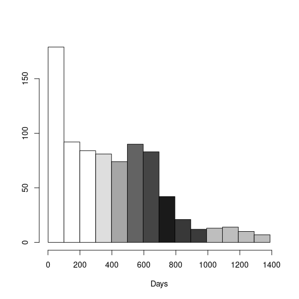
The average (over uncensored observations) unemployment duration of treatment group members is 20 days lower than that of their control group counterparts. The proportion of censored observations is around 32%. The mode of the unemployment duration (when it is observed) is 26 days and the median is 361 days. A large number of observations of duration is around 600 days. This corresponds to the time around which many follow-up interviews were held. Beyond this point, almost all observations are censored.

To compute the estimator $\hat{\beta}(u)$ while avoiding local minima, we initialize the optimization algorithm at 1,000 random initialization points. We then select the estimate which minimizes the objective function among the resulting vectors. This procedure is applied for each $u\in\{0.1,0.2,...,0.9\}$. We can use the results of the analysis to conduct an informal joint test of our assumptions. Indeed, recall that our identification conditions at $u$ include the fact that

(see Section 3.3). If our identification and estimation conditions were satisfied at $u$, then $\widehat{\beta}(u)$ would converge to $\beta(u)$ and therefore, by (6.1), we should expect to have

with high probability. Since (6.2) does not hold for the quantiles $u\in\{0.7,0.8,0.9\}$, we conclude that our conditions are not satisfied for these quantiles. In order to construct confidence intervals, we use the bootstrap approach discussed in Section 4.1.

We report the estimates and the 95% (percentile bootstrap) confidence intervals for $\beta_{2}$ and $\beta_{3}$ in Figure 1. The results indicate that the treatment has a significant and negative effect on $T$. In addition, there is some evidence that the treatment effect varies by quantile. We find a significant and negative effect of age on unemployment duration. In Section S3 of the supplementary material, we include a table reporting the exact values of the estimates and the bounds of the confidence intervals.

Financial support from the European Research Council (2016-2022, Horizon 2020 / ERC grant agreement No. 694409) is gratefully acknowledged.

References

- Abadie et al. (2002) Abadie, A., J. Angrist, and G. Imbens (2002). Instrumental variables estimates of the effect of subsidized training on the quantiles of trainee earnings. Econometrica 70, 91–117.
- Angrist et al. (1996) Angrist, J. D., G. W. Imbens, and D. B. Rubin (1996). Identification of causal effects using instrumental variables. Journal of the American Statistical Association 91, 444–455.
- Beyhum et al. (2022) Beyhum, J., J.-P. Florens, and I. Van Keilegom (2022). Nonparametric instrumental regression with right censored duration outcomes. Journal of Business & Economic Statistics 40, 1034–1045.
- Bickel and Freedman (1981) Bickel, P. J. and D. Freedman (1981). Asymptotic theory for the bootstrap. Annals of Statistics 9, 1196–1217.
- Blanco et al. (2020) Blanco, G., X. Chen, C. A. Flores, and A. Flores-Lagunes (2020). Bounds on average and quantile treatment effects on duration outcomes under censoring, selection, and noncompliance. Journal of Business & Economic Statistics 38, 901–920.
- Blundell and Powell (2007) Blundell, R. and J. L. Powell (2007). Censored regression quantiles with endogenous regressors. Journal of Econometrics 141, 65–83.
- Bose and Chatterjee (2018) Bose, A. and S. Chatterjee (2018). U-statistics, Mm-estimators and Resampling. Berlin: Springer.
- Brown and Wegkamp (2002) Brown, D. J. and M. H. Wegkamp (2002). Weighted minimum mean-square distance from independence estimation. Econometrica 70, 2035–2051.
- Buchinsky and Hahn (1998) Buchinsky, M. and J. Hahn (1998). An alternative estimator for the censored quantile regression model. Econometrica 66, 653–671.
- Centorrino and Florens (2021) Centorrino, S. and J.-P. Florens (2021). Nonparametric estimation of accelerated failure-time models with unobservable confounders and random censoring. Electronic Journal of Statistics 15, 5333 – 5379.
- Chen and Wang (2020) Chen, S. and Q. Wang (2020). Semiparametric estimation of a censored regression model with endogeneity. Journal of Econometrics 215, 239–256.
- Chernozhukov et al. (2015) Chernozhukov, V., I. Fernández-Val, and A. E. Kowalski (2015). Quantile regression with censoring and endogeneity. Journal of Econometrics 186, 201–221.
- Chernozhukov and Hansen (2005) Chernozhukov, V. and C. Hansen (2005). An IV model of quantile treatment effects. Econometrica 73, 245–261.
- Chernozhukov and Hong (2002) Chernozhukov, V. and H. Hong (2002). Three-step censored quantile regression and extramarital affairs. Journal of the American Statistical Association 97, 872–882.
- De Backer et al. (2019) De Backer, M., A. El Ghouch, and I. Van Keilegom (2019). An adapted loss function for censored quantile regression. Journal of the American Statistical Association 114, 1126–1137.
- De Backer et al. (2020) De Backer, M., A. El Ghouch, and I. Van Keilegom (2020). Linear censored quantile regression: A novel minimum-distance approach. Scandinavian Journal of Statistics 47, 1275–1306.
- Fève et al. (2018) Fève, F., J.-P. Florens, and I. Van Keilegom (2018). Estimation of conditional ranks and tests of exogeneity in nonparametric nonseparable models. Journal of Business & Economic Statistics 36, 334–345.
- Fitzenberger (1997) Fitzenberger, B. (1997). A guide to censored quantile regressions. Handbook of Statistics 15, 405–437.
- Frandsen (2015) Frandsen, B. R. (2015). Treatment effects with censoring and endogeneity. Journal of the American Statistical Association 110, 1745–1752.
- Giacomini et al. (2013) Giacomini, R., D. N. Politis, and H. White (2013). A warp-speed method for conducting Monte Carlo experiments involving bootstrap estimators. Econometric Theory 29, 567–589.
- Gill (1983) Gill, R. (1983). Large sample behaviour of the product-limit estimator on the whole line. Annals of Statistics, 49–58.
- Hong and Tamer (2003) Hong, H. and E. Tamer (2003). Inference in censored models with endogenous regressors. Econometrica 71, 905–932.
- Honore et al. (2002) Honore, B., S. Khan, and J. L. Powell (2002). Quantile regression under random censoring. Journal of Econometrics 109, 67–105.
- Khan and Powell (2001) Khan, S. and J. L. Powell (2001). Two-step estimation of semiparametric censored regression models. Journal of Econometrics 103, 73–110.
- Khan and Tamer (2009) Khan, S. and E. Tamer (2009). Inference on endogenously censored regression models using conditional moment inequalities. Journal of Econometrics 152, 104–119.
- Kosorok (2008) Kosorok, M. R. (2008). Introduction to empirical processes and semiparametric inference. Berlin: Springer.
- Lo and Singh (1986) Lo, S.-H. and K. Singh (1986). The product-limit estimator and the bootstrap: some asymptotic representations. Probability Theory and Related Fields 71, 455–465.
- Martinussen et al. (2019) Martinussen, T., D. Nørbo Sørensen, and S. Vansteelandt (2019). Instrumental variables estimation under a structural Cox model. Biostatistics 20, 65–79.
- Milnor and Weaver (1997) Milnor, J. and D. W. Weaver (1997). Topology from the differentiable viewpoint, Volume 21. Princeton: Princeton university press.
- Nelder and Mead (1965) Nelder, J. A. and R. Mead (1965). A simplex method for function minimization. The Computer Journal 7, 308–313.
- Newey and McFadden (1994) Newey, W. K. and D. McFadden (1994). Large sample estimation and hypothesis testing. Handbook of Econometrics 4, 2111–2245.
- Peng (2021) Peng, L. (2021). Quantile regression for survival data. Annual Review of Statistics and its Application 8, 413–437.
- Peng and Huang (2008) Peng, L. and Y. Huang (2008). Survival analysis with quantile regression models. Journal of the American Statistical Association 103, 637–649.
- Poirier (2017) Poirier, A. (2017). Efficient estimation in models with independence restrictions. Journal of Econometrics 196, 1–22.
- Portnoy (2003) Portnoy, S. (2003). Censored regression quantiles. Journal of the American Statistical Association 98, 1001–1012.
- Powell (1984) Powell, J. L. (1984). Least absolute deviations estimation for the censored regression model. Journal of Econometrics 25, 303–325.
- Powell (1986) Powell, J. L. (1986). Censored regression quantiles. Journal of Econometrics 32, 143–155.
- Richardson et al. (2017) Richardson, A., M. G. Hudgens, J. P. Fine, and M. A. Brookhart (2017). Nonparametric binary instrumental variable analysis of competing risks data. Biostatistics 18, 48–61.
- Sant’Anna (2016) Sant’Anna, P. H. (2016). Program evaluation with right-censored data. arXiv preprint arXiv:1604.02642.
- Sant’Anna (2021) Sant’Anna, P. H. (2021). Nonparametric tests for treatment effect heterogeneity with duration outcomes. Journal of Business & Economic Statistics 39, 816–832.
- Tchetgen Tchetgen et al. (2015) Tchetgen Tchetgen, E. J., S. Walter, S. Vansteelandt, T. Martinussen, and M. Glymour (2015). Instrumental variable estimation in a survival context. Epidemiology 26, 402.
- Torgovitsky (2017) Torgovitsky, A. (2017). Minimum distance from independence estimation of nonseparable instrumental variables models. Journal of Econometrics 199, 35–48.
- U.S. Department of Labor (1993) U.S. Department of Labor (1993). The National Job Training Partnership Act Study: Dataset. W.E. Upjohn Institute for Employment Research. http://hdl.handle.net/1902.1/IOJHHXOOLZ.
- Van der Vaart and Wellner (1996) Van der Vaart, A. W. and J. A. Wellner (1996). Weak Convergence and Empirical Processes. Springer Series in Statistics. New York: Springer-Verlag.
- Wang and Wang (2009) Wang, H. J. and L. Wang (2009). Locally weighted censored quantile regression. Journal of the American Statistical Association 104, 1117–1128.
- Wang et al. (2022) Wang, L., E. Tchetgen Tchetgen, T. Martinussen, and S. Vansteelandt (2022). Instrumental variable estimation of the causal hazard ratio (with discussion). Biometrics (forthcoming).
- Wang and Chen (2021) Wang, Q. and S. Chen (2021). Moment estimation for censored quantile regression. Econometric Reviews 40, 815–829.
- Wei et al. (2021) Wei, B., L. Peng, M.-J. Zhang, and J. P. Fine (2021). Estimation of causal quantile effects with a binary instrumental variable and censored data. Journal of the Royal Statistical Society: Series B (Statistical Methodology) 83, 559–578.
- Yang et al. (2018) Yang, X., N. N. Narisetty, and X. He (2018). A new approach to censored quantile regression estimation. Journal of Computational and Graphical Statistics 27, 417–425.
Appendix A Proof of identification results
A.1 Proof of Theorem 3.1
By (3.1), is a solution of
Now suppose is another solution. We obtain
Denote by the quantity Then, the last equality can be rewritten as
Now, by definition of , we have for all and . This implies that for all , it holds that , where is the differential of evaluated at . Therefore, using Fubini’s Theorem and the definition of given in Section 3.2.1, the last equation takes also the form
The strong completeness of by given implies that, almost everywhere,
and so and almost surely. Taking the expected value on both sides we obtain , since is full rank by hypothesis.
A.2 Proof of Theorem 3.2
The proof is inspired by that of Theorem 2 in Chernozhukov and Hansen 2005. Consider the two iso-probability curves and , defined as
Under Assumption 2.1, the curves and satisfy the differential equations
Therefore, the slopes at a given point point of the curves and are, respectively,