Triage of the Gaia DR3 astrometric orbits. I. A sample of binaries with probable compact companions2022Triage of the Gaia DR3 astrometric orbits. I. A sample of binaries with probable compact companions–References
Abstract\par
In preparation for the release of the astrometric orbits of Gaia, Shahaf et al. (2019) proposed a triage technique to identify astrometric binaries with compact companions based on their astrometric semi-major axis, parallax, and primary mass. The technique requires the knowledge of the appropriate mass-luminosity relation to rule out single or close-binary main-sequence companions. The recent publication of the Gaia DR3 astrometric orbits used a schematic version of this approach, identifying astrometric binaries that might have compact companions. In this communication, we return to the triage of the DR3 astrometric binaries with more careful analysis, estimating the probability for its astrometric secondary to be a compact object or a main-sequence close binary. We compile a sample of systems with highly-probable non-luminous massive companions, which is smaller but cleaner than the sample reported in Gaia DR3. The new sample includes candidates to be black-hole systems with compact-object masses larger than . The orbital-eccentricity–secondary-mass diagram of the other systems suggests a tentative separation between the white-dwarf and the neutron-star binaries. Most white-dwarf binaries are characterized by small eccentricities of about and masses of , while the neutron star binaries display typical eccentricities of and masses of .
Keywords: \par
astrometry – binaries: general – stars: white dwarfs – stars: neutron – stars: black holes1 \parIntroduction
The population of binaries with white-dwarf (WD), neutron-star (NS), or black-hole (BH) companions is of great interest. It sheds light on the properties of the binaries for which the more massive primary component completed its main-sequence (MS) phase and on the dramatic processes accompanying the transition into a compact object (heger03;\par Cerda-Duran &Elias-Rosa 2018, e.g.,). Astrometry is an important tool to study this population, as it is sensitive to binaries with orbital periods of the order of a few years, depending on the binary distance, which corresponds to orbital separations to which other techniques, spectroscopy or photometry, are less sensitive (Jorissen &Frankowski 2008, e.g.,). Furthermore, unlike spectroscopic binaries for which the orbital inclination is not known, the compact-object mass in astrometric binaries can be determined, and the three types of compact objects can, in principle, be distinguished (Halbwachs et al. 2022, e.g.,).
The Gaia astrometric space mission (Gaia Collaboration et al. 2016) provides a promising detection channel, as it is expected to detect an unprecedentedly large number of astrometric binaries. For example, theoretical studies predict that the Gaia mission carries the potential of discovering hundreds of binaries with non-interacting BHs in orbital periods years (breivik17;\par mashian17;\par yamaguchi21;\par janssens22;\par Chawla et al. 2022, e.g., ). NSs and WDs should be even more frequent (Fryer et al. 2012, e.g.,). Note, however, that the stringent selection criteria imposed on the DR3 sample of astrometric binaries (Halbwachs et al. 2022, see ), designed to reduce the contamination of the astrometric catalogue by spurious signals, probably excluded many of these systems, impairing the detection of the compact objects.
In preparation for the release of the astrometric orbits of Gaia, Shahaf et al. 2019 proposed a triage technique to identify astrometric binaries that have compact companions based on their derived semi-major axis, parallax, orbital period and the estimated primary mass. The technique requires the knowledge of the proper mass-luminosity relation (MLR) to rule out a single or a close-binary MS companion. Indeed, the DR3 binary release (36, hereafter NSS — Non-Single Stars) used a schematic version of this approach, with the MLR of Pecaut &Mamajek 2013, to identify astrometric binaries with compact companions (see also andrews19;\par Andrew et al. 2022, for a different approach).
In this communication, we return to the triage of the DR3 astrometric binaries with a more careful analysis that uses a more conservative MLR to identify compact-secondary binaries based on a suit of MIST isochrone grids.1\par1\par MESA Isochrones &Stellar Tracks. See waps.cfa.harvard.edu/MIST/. We derive a less contaminated catalogue of compact companions, identifying astrometric binaries with WD, NS or BH companions.
The paper is structured as follows: In Section 2 \parAstrometric Triage we briefly describe our astrometric triage scheme and discuss the effect of stellar age and composition on this technique. In Section 3 \parTriage of Gaia binaries we present the triage of Gaia DR3 binaries, provide a list of class-membership probabilities, and compile a sample of systems that are very likely to host a compact object in Section 4 \parHighly-probable class-III systems. In Section 5 \parA tentative distinction between WD and NS candidates we show some of the emerging properties of our compact-object sample. Finally, in Section 6 \parSummary and Discussion we briefly discuss the sample and preliminary findings and propose some ideas for future work.
2 \parAstrometric Triage
In this section, we re-discuss the astrometric triage introduced by Shahaf et al. 2019, with a focus on using the appropriate MLR for MS stars.
Consider an astrometric binary with an angular semi-major axis . For an unresolved binary, reflects the motion of the centre-of-light around the binary centre-of-mass. In cases where the more luminous primary star is significantly brighter than its secondary companion, the photo-centre of the system is located near the primary star’s position. This could happen, for example, if the secondary is a faint sub-stellar companion or a compact object. On the other hand, if both components are luminous, the photo-centre is located near the centre-of-mass of the binary, up to a point where no astrometric orbit can be detected.
Shahaf et al. 2019 presented the astrometric mass ratio function (AMRF),
where and are the orbital period and parallax, and is the mass of the primary, more luminous, star. can be determined for every astrometric binary for which is known.
The unknown mass ratio is linked to AMRF via
where is the luminosity ratio between the two components. The term inside the parenthesis in equation (2 \parAstrometric Triage) accounts for the fact that we follow the orbit of the photo-centre, rather than that of the primary star (see, for example, van de Kamp 1975); assuming the mass-luminosity relation is superlinear, and this term is non-negative.
Shahaf et al. 2019 showed that whenever the luminosity ratio of the two possible MS stars can be expressed as a function of the mass ratio, , one is able to place some constraints on the nature and properties of the faint companion in the binary system. A lower estimate for the mass ratio is obtained by assuming that the secondary companion is non-luminous, namely, plugging into equation (2 \parAstrometric Triage). Under this assumption, the AMRF is a function of the mass ratio alone.
The minimal mass ratio, is a root of the polynomial . Since is a positive number, the minimal mass ratio is unique and can be obtained analytically (heacox95;\par shahaf17;\par Andrew et al. 2022, e.g.,). The corresponding minimal secondary mass, i.e., the mass of the companion assuming that it does not emit light, is given by
This lower limit on the mass may, in many cases, constrain the compact object’s nature. However, this can only be done if we rule out the possibility of a single MS secondary or a companion who is by itself a close MS binary.
2.1 \parAMRF classification
To illustrate the triage approach, we plot in Figure Triage of the Gaia DR3 astrometric orbits. I. A sample of binaries with probable compact companions two theoretical AMRF curves as a function of the mass ratio , for and MS primary stars. The dotted (lower) curves in the two panels present binaries with a single MS secondary; the dashed (upper) curves triple systems, with a close equal-mass MS binary as the astrometric secondary; and the solid curves binaries with a non-luminous companion. The dotted and dashed lines were derived with the Gaia G-band MLR of Pecaut &Mamajek 2013.
Binaries with MS companions have to reside on the lower dotted curves, with a position that depends on the mass ratio of the astrometric binary. Triple systems with close-binary MS companions could be located anywhere below the upper dashed line, depending on the mass ratio of the close binary. Only triple systems with equal-mass close-binary companions have to be on the upper dashed line, with a position that depends on the wide-binary mass ratio. Binaries with compact companions have to reside on the continuous curve. Note that the positions of realistic systems do not necessarily fall on the expected position. This is because the shape of the distinguishing lines is affected by the accuracy of the assumed MLR, and because a binary position on the diagram is affected by the measurements uncertainties.
The AMRF theoretical curves have maximal values — for the single MS secondary and for the triple-system curve. These values, which depend on the primary mass, are noted in the figure by dots and squares. Any wide binary with probably has a compact companion. If the companion is a single object, the system has to reside on the continuous curve. In such a case, the companion mass can be derived from the value of .
In the general case, though, one cannot determine the value of , even if the primary mass is known, because the luminosity of the secondary is unknown. Therefore, to identify unresolved astrometric binaries that are likely to host a compact object as their faint companion, Shahaf et al. 2019 divided the astrometric binaries into three classes, based on their measured AMRF value, :
-
Class-I binaries (), where the companion is most likely a single MS star. The class-I parameter space is shown as a crisscrossed area in Figure 2 \parAstrometric Triage.
-
Class-II binaries (), where the companion cannot be a single MS star, but can be either a MS close binary or a compact object. The class-II parameter space is denoted with slanted lines.
-
Class-III binaries (), where the companion cannot be a single MS star nor a close MS binary; these systems are likely to host a compact object secondary. The class-III parameter space is highlighted by small circles.
Figure Triage of the Gaia DR3 astrometric orbits. I. A sample of binaries with probable compact companions demonstrates that the limiting values and vary as a function of . Figure 2 \parAstrometric Triage shows the limiting AMRF values as a function of the primary mass. We added in Figure 2 \parAstrometric Triage purple and light-blue stripes that illustrate the expected values of WDs, at , and NSs, at .
Note that the locations of binaries with primaries and NS companions are all in the class-III region, making their identification relatively simple. The WD stripe, on the other hand, is only partially above the curve. This implies that only binaries with massive WDs can be identified as such, while binaries with low-mass WDs and relatively massive primaries will escape detection. We will come back to this point in an accompanying paper.
2.2 \parRe-consideration of class-II and class-III limits
The AMRF limits depend on the assumed MLR, which in turn depends on the age and chemical composition of the specific binary. The observed MLR of Pecaut &Mamajek 2013 used in Figure Triage of the Gaia DR3 astrometric orbits. I. A sample of binaries with probable compact companions and 2 \parAstrometric Triage is an averaged relation, taken over the distribution of ages and compositions in the Solar neighborhood. While this relation can properly describe the population of stars in the field, this is not necessarily the case when considering two stars in a particular binary system. Assuming the two stars were formed at the same time and have the same composition, their relative flux contribution follows some specific isochrone track rather than the local averaged MLR.
To demonstrate this point Figure 2 \parAstrometric Triage presents two curves for two different populations: a young population, with age of Myr and (a dashed-blue curve), an old population of Gyr and (dashed-red curve). To derive the first two curves we simulated a synthetic stellar population using ArtPop package2\par2\par See the online documentation at artpop.readthedocs.io (Greco &Danieli 2021) and the MIST isochrone grids. The figure also displays the (upper) curve of Figure Triage of the Gaia DR3 astrometric orbits. I. A sample of binaries with probable compact companions (dashed-gray curve), based on Pecaut &Mamajek 2013 MLR, which was used by 36.
Figure 2 \parAstrometric Triage shows that the limit used by 36 often underestimates the limiting AMRF values separating between class-II and -III binaries. Therefore, we have adopted a more conservative classification curve based on the upper envelope of an ensemble of models generated over various stellar ages and metallicities. As opposed to the 36 classification curve, our curve provides reliable and curves that can be used regardless of the underlying age and metallicity of the binary. We elaborate on the derivation of the curves in the following subsection.
2.3 \parAdopted classification limits
In Section 2.2 \parRe-consideration of class-II and class-III limits we show that the shape of and depends on the age and composition of the stars in the binary system. In light of this claim, a plausible course of action would be to classify each binary while considering its particular age, iron abundance, and corresponding uncertainty estimates.
However, the Flame stellar ages tend to have large uncertainties (creevey22;\par Babusiaux et al. 2022) and the GSP-phot metallicities are probably biased and require further calibration (Andrae et al. 2022). Furthermore, these values are provided by Gaia only to about half of the sample of astrometric binaries. As a result, and after attempting to incorporate these values, we concluded that the use of individual age and metallicity estimates is not efficient. Instead, we opted to derive a ‘global’ limiting curve that can provide a conservative estimate for the values for the classification, even when the age and composition are not well constrained.
To do so, we generated a set of and curves, spanning from to in and to in [Fe/H]. The spacing in both grids is dex. Based on this set of limiting values, we generated a new limiting curve that follows the outer envelope of all curves in our grid. To do so, we used the percentile of all curves for a given mass value and smoothed the resulting envelope with a moving average with a width of .
Theoretical models are known to estimate the radii of M-dwarfs inaccurately (Morrell &Naylor 2019, e.g.,). Therefore, for primary stars less massive than , instead of using the upper envelope of the theoretical models, we used the one based on the Pecaut &Mamajek 2013 MLR. We added a positive constant to this low-mass limiting curve to ensure that the final curve is continuous. The resulting limiting curve is plotted, as solid black lines, along with all the models used in our ensemble, in Figure 2.3 \parAdopted classification limits. A lookup table with the values of the limiting curves is provided in the supplementary material.
Figure 2.3 \parAdopted classification limits demonstrates how the limiting curves computed based on the Pecaut &Mamajek 2013 MLR follow the general trend of those generated using MIST isochrones. The figure also shows that some MIST-based curves significantly deviate from this trend. For primary stars more massive than , these deviations are mostly caused by mildly evolved stars, that are on the verge of leaving the MS. On the other hand, for primaries less massive than the deviations mostly represent young stars of high metallicity.

3 \parTriage of Gaia binaries
Equipped with a more conservative threshold for class-III binaries, we now turn to re-consider the Gaia astrometric binaries. First, we derive a slightly smaller sample of astrometric binaries by vetting the targets based on the reported orbital parameters. Then, we obtain the probability of each binary being in class-II or class-III, given their orbital parameters and uncertainties.
3.1 \parSample selection
We first queried the Gaia database for astrometric binaries with MS primary stars that have mass estimate, according to the following conditions:
-
nss solution type is Orbital or AstroSpectroSB1;
-
bit index is or ;
-
binary masses catalogue m1 ref is IsocLum; and
-
binary masses catalogue combination method is
-
Orbital+M1 or AstroSpectroSB1+M1.
The first two conditions require that the astrometric orbit was derived from the primary processing pipeline and has all orbital parameters fitted. The following two conditions require that a primary mass estimate exists for the system and that its primary star was classified by as an MS star. For details regarding the derivation of the masses, see section 5.1 of 36. This procedure left a total of targets in the sample.
We then applied the Halbwachs et al. 2022 criteria on the eccentricity error, parallax significance, , and astrometric solution significance, .
-
;
-
; and
-
.
These additional cuts, which were supposed to reduce the number of spurious orbital solutions in the sample, removed only a few additional systems, and we were left with stars with mass estimates. Out of this sample, orbits were obtained based on joint-modelling of the astrometric and spectroscopic data (AstroSpectroSB1) and the rest considered the astrometric data alone (Orbital).
Next, we opted to exclude systems with poorly constrained Thiele-Innes coefficients. A full description of these coefficients and the required formulae for using them to derive the angular semi-major axis can be found in Halbwachs et al. 2022. We required, somewhat arbitrarily, that the quadratic mean of the relative uncertainty in , , , and Thiele-Innes coefficients will be smaller than , namely
This step was taken to ensure that our classification probability estimates (see below) properly converge and left orbits in the cleaned sample.
Finally, we opted to exclude targets with orbital periods longer than the time span of the data analyzed by Gaia DR3. We, therefore, removed systems with orbital periods longer than days. We were eventually left with systems in our cleaned sample. This sample includes AstroSpectroSB1 orbital and Orbital solutions. Our additional selection criteria, therefore, slightly favor AstroSpectroSB1 solutions over Orbital ones.
3.2 \parDistribution of the derived AMRF
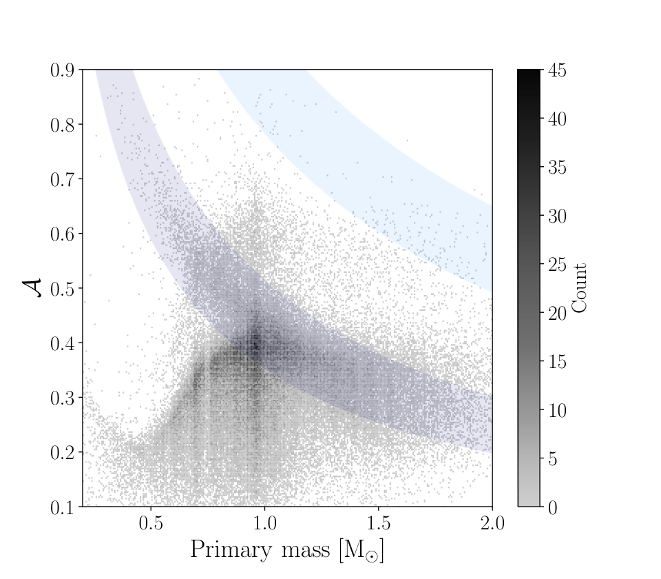
Figure 3.2 \parDistribution of the derived AMRF presents a density plot of the cleaned sample on the AMRF–primary-mass plane.
The figure displays a prominent vertical concentration at about , probably due to the overabundance of solar-type stars in the Gaia sample. The vertical stripe has a clear maximum density at , which seems to leak over neighbouring masses, at a range of between and . The position and shape of this feature are in line with the expected values of , shown in the bottom panel of Figure 2.3 \parAdopted classification limits. The occurrence of systems at this region of parameters is probably enhanced by an observational bias: for an MS binary, the AMRF attains its maximal value, together with the maximal size of the photo-centric orbit. As a result, Gaia probably favours the detection of these systems.
An additional feature of Figure 3.2 \parDistribution of the derived AMRF is a well-separated cluster of relatively high AMRF values, centered at for primary masses of . The position of this cluster is consistent with the expected range of values of , shown in the top panel of Figure 2.3 \parAdopted classification limits. A plausible claim is that this cluster is comprised of triple systems with close equal-mass MS binaries as the astrometric secondaries.
The diagram also shows an excess of systems with high AMRF values, between and , located within the purple stripe, probably consisting of WD companions, and a few binaries that might have NS companions (see below).

3.3 \parClassification probability
We move now to dividing the cleaned sample into the three classes of Section 2 \parAstrometric Triage. Because of the uncertainties of the theoretical boundaries and the uncertainties of the primary mass and , our classification is of probabilistic nature. We derive three probabilities:
using Monte-Carlo experiments. To consider the uncertainties of the orbital elements, we randomly drew random instances of the Thiele-Innes parameters, parallax, period, eccentricity and primary mass. The sampling was performed while considering the uncertainties and covariance between the parameters, as reported in the Gaia catalogue.
As proposed by Shahaf et al. 2019, the values of the AMRF and primary mass determine the classification of the binary. We calculated , , and for each draw, and estimated the class-III probability by
where is the number of instances for which is larger than (see, for example, Davison &Hinkley 1997). The class-II membership probability, , was estimated similarly. For brevity, we do not use the ‘hat’ superscript in the following. We emphasize that whenever membership probability is discussed, we refer to our bootstrap-based estimate, derived according to equation (3.3 \parClassification probability), as described above.
A list of the Pr II and Pr III classification probabilities for all targets in our sample is provided in Table 3.3 \parClassification probability. The class-I membership probability, Pr I, can be derived using the two other class probabilities, the number of Monte-Carlo samples, , and equation (3.3 \parClassification probability). Histograms of the classification probabilities are plotted in Figure 3.2 \parDistribution of the derived AMRF.
Figure 3.2 \parDistribution of the derived AMRF displays the distribution of Pr III in the AMRF–primary-mass plane. Each bin in the diagram is colour coded according to its mean Pr III value. A concentration of high-Pr III systems is located above the curve, and appears in black. A stripe of systems with high to intermediate class-III probability follows the expected WD envelope. The analysis of this sub-sample of possible binaries with WD companions is deferred to a follow-up study.
Figure 3.2 \parDistribution of the derived AMRF also suggests that for primary stars less massive than , the limiting values calculated according to the MIST models tend to underestimate the transition between class-I and -II systems. This is in accord with a reported discrepancy between the empirically estimated and the theoretically expected M-dwarf radii (Morrell &Naylor 2019, e.g.,). As described above, we rectified our limiting curves for primaries less massive than , so that they were not severely affected by this discrepancy (also see Figure 2 \parAstrometric Triage).
| Source ID | Pr II | Pr III | |||
|---|---|---|---|---|---|
| () | () | (%) | (%) | ||
| 33711199137024 | 0.95 | 56.198 | 8.800 | ||
| 148953761446272 | 1.25 | 0.836 | 0.001 | ||
| 301614079110400 | 1.01 | 75.302 | 24.699 | ||
| 858688517149056 | 1.22 | 0.001 | 0.001 | ||
| 1729398647131392 | 0.56 | 0.072 | 0.001 | ||
| 2488955023504768 | 0.49 | 0.001 | 0.001 | ||
| 3019435024120576 | 0.65 | 36.036 | 2.885 | ||
| 3205080690546176 | 0.85 | 19.105 | 0.006 | ||
| 3334754343120640 | 0.64 | 6.864 | 93.137 | ||
| 3616877859431808 | 0.93 | 10.752 | 0.001 |
| Source ID | Period | Eccentricity | label | note | ||||
|---|---|---|---|---|---|---|---|---|
| () | () | (day) | ||||||
| 4373465352415301632 | 1.0 | 13.6 | 1.2 | BH | Gaia BH1 (El-Badry et al. 2022) | |||
| 6281177228434199296 | 1.0 | 24.3 | 0.6 | BH | refuted (El-Badry et al. 2022) | |||
| 3509370326763016704 | 0.7 | 76.1 | 0.2 | BH | refuted (El-Badry et al. 2022) | |||
| 6802561484797464832 | 1.2 | 6.8 | 0.3 | BH | refuted (El-Badry et al. 2022) | |||
| 3263804373319076480 | 1.0 | 18.1 | 2.1 | BH | AstroSpectroSB1 | |||
| 6601396177408279040 | 1.0 | 10.8 | 1.1 | BH | ||||
| 6328149636482597888 | 1.1 | 89.9 | 3.8 | BH | ||||
| 6588211521163024640 | 1.1 | 10.4 | 4.2 | BH | ||||
| 4482912934572480384 | 0.9 | 19.3 | 0.7 | NS | ||||
| 5580526947012630912 | 1.2 | 12.9 | 0.1 | NS |
4 \parHighly-probable class-III systems
We now define a sample of systems likely to host compact companions, applying the Benjamini &Hochberg 1995 false-discovery rate (FDR) approach, designed to control the expected proportion of false discoveries. In the present work context, false discoveries are systems that are wrongfully identified as class-III binaries.
We set , the upper limit on the expectancy values of the false discovery rate, to
which yields systems in this sub-sample, which we refer to as the class-III sample henceforth. Accordingly, only () or fewer binaries are expected to be wrongly identified as class-III systems.
A discussion of what constitutes a false discovery in the context of this work is given in Section 6 \parSummary and Discussion. The selection criterion we used is equivalent to setting a minimal class-III probability of , i.e., only out of the Monte-Carlo instances fell below the limit. A list of the selected class-III binaries is given in Table 3.3 \parClassification probability.
Most of these systems, if their orbits are valid, contain compact secondaries. Therefore, we can derive their masses and possibly distinguish between the WD, NS or BH companions. However, we stress the possibility that erroneous orbital fits might contaminate the sample, particularly when considering a sample of rare candidates. We therefore advocate that the validity of these orbits should be assessed externally (see the caveats discussion in Section 6 \parSummary and Discussion).
The proportion of AstroSpectroSB1 orbits in the class-III sample is lower than that of the entire sample; out of the 177 systems, only seven binaries have a joint astrometric and spectroscopic orbital solution. This is probably because the median G-band magnitude of the class-III systems is , magnitudes fainter than the median of the entire clean-astrometric sample. As we know, the Gaia RVS measurements are limited to bright stars, with a limit at mag. The difference in apparent magnitude between the clean sample and the class-III sample is associated with the mass bias of the triage scheme. As detailed in Sections 2 \parAstrometric Triage and 6 \parSummary and Discussion, the triage is more sensitive to low-mass stars with WD companions.
4.1 \parComparison with the NSS candidates
Gaia DR3 36 includes a list of class-III systems, while our list includes only binaries. The difference emanates from:
-
vetting the quality of the orbital solution,
-
conservatively estimating the limiting curve, and
-
setting a high-purity threshold on Pr III.
As a result of the different vetting, only systems of the 36 sample are included in our cleaned sample (see Section 3.1 \parSample selection). While all these systems have , only were classified here as highly probable class-III systems. We attribute the difference to our conservative approach in setting the limiting classification value, .
There are systems in our class-III sample that do not appear in the 36 class-III sample. These systems were not included by 36 because their significance value is smaller than , the limit they adopted for considering valid orbits. As explained above, we used a different limit, which we believe is more appropriate for our purpose, and allowed us to include them in the analysis.
4.2 \parComparison with the Andrews et al. (2022) candidates
Another catalogue of NS and BH candidates in Gaia DR3 was recently published by Andrews et al. 2022, based on their derived mass function (see equation 5.1 \parIncompleteness of the compact object sample); out of this sample, of are also included in our class-III sample. The remaining systems were rejected in our early stage of initial sample selection (see Section 3.1 \parSample selection) — six have orbital periods longer than day, three do not have a primary mass estimate in the binary masses table, and one system did not meet our Thiele-Innes relative uncertainty criterion.
All systems shared by both samples appear in our class-III sample. Of these, the companion of Gaia DR3 6328149636482597888 has a mass larger than and is considered a BH candidate (Table 3.3 \parClassification probability). The remaining are NS candidates, with companion masses between and .
4.3 \parComparison with El-Badry et al. (2022) candidates
El-Badry et al. 2022 also compiled a list of BH candidates based on Gaia DR3 astrometric orbits, using the derived mass ratio of the systems. Their final list included six targets, including the first two systems of our Table 3.3 \parClassification probability class-III sample. Four other systems do not appear on our list, since their orbital periods are longer than day.
El-Badry et al. 2022 further embarked on an efficient spectroscopic follow-up campaign to validate their orbital solutions. The first target of Table 3.3 \parClassification probability, Gaia DR3 4373465352415301632 (Gaia BH1 henceforth), was validated by their spectroscopic follow-up campaign. As per the writing of this text, Gaia BH1 is the only bona-fide BH detected in DR3 data. The properties of this system are somewhat unexpected. We refer to El-Badry et al. 2022 for a detailed discussion on its properties and the implications of its discovery. The second target shared by both candidate lists is Gaia DR3 6281177228434199296. As opposed to Gaia BH1, this system was refuted by the follow-up campaign.
El-Badry et al. 2022 also monitored, and consequentially refuted, two additional systems identified in our work: Gaia DR3 3509370326763016704 and 6802561484797464832. Hence, out of the first four BH candidates presented in Table 3.3 \parClassification probability, one was confirmed and three can be deemed as spurious, based on follow-up observations. See the caveats discussion in Section 6 \parSummary and Discussion.
5 \parA tentative distinction between WD and NS candidates
The distinction between the WD and the NS in our catalogue is not trivial because some WDs were found by previous studies to have masses greater than the masses of the least massive NSs (martinez15;\par Caiazzo et al. 2021, e.g.,). Furthermore, some compact secondaries with mass typical of NS might be close binaries composed of two WDs. Nevertheless, one might be helped in separating the two populations if some orbital properties of the WD binaries statistically differ from those of the NS binaries.
To explore this possibility, we plot in Figure 5 \parA tentative distinction between WD and NS candidates the orbital eccentricity versus the secondary mass for all objects in our compact-object sample, except for the eight systems with masses larger than . The figure suggests two clusters of binaries — one with the typical WD mass of and low eccentricity, and the other with the typical NS mass of and higher eccentricity.
To tentatively divide the sample into WD and NS candidates, we fitted the eccentricity--secondary-mass diagram with a component Gaussian mixture model.3\par3\par This was done using Scikit-learn GaussianMixture module. The mean Silhouette similarity score (Rousseeuw 1987) was used to select the number of components in the mixture.4\par4\par See the Scikit-learn Silhouette score function. The score was calculated using the cosine-distance metric, to favour the masses-eccentricities relation over their actual values. The Silhouette score became negative when using more than three Gaussian components, which indicates that the resulting clusters overlap. Nevertheless, we emphasise that this is merely a tentative classification, and refer the readers to the caveats discussion in Section 6 \parSummary and Discussion.
We used two components to describe the distribution of the low-mass circularized systems (‘WD cluster’) and another component for the massive eccentric ones (‘NS cluster’). The WD cluster is described by
where represents a normal distribution, its first entry representing the derived expectancy for the secondary mass in Solar units (top) and the eccentricity (bottom), and the second entry is the corresponding covariance matrix. Similarly, the NS cluster is described by
The odds ratio between the two clusters is , in favour of the WD cluster.
The central regions of the two clusters are presented as thin purple lines in Figure 5 \parA tentative distinction between WD and NS candidates. The points are coloured by their classification: white circles represent the objects in the WD cluster, and the blue circles represent the objects in the NS cluster. The distinction between the two clusters was made according to their cluster-membership probabilities, and , of the Gaussian mixture model. The targets with were labeled as NS cluster members; the targets in the complement set, with , were labeled as members of the WD cluster. The BH candidates, with masses larger than , are not included in any of the two classes.
Figure 5 \parA tentative distinction between WD and NS candidates presents the mass distribution of the secondary masses, overlaid with the marginal probability density function of the Gaussian mixture of Figure 5 \parA tentative distinction between WD and NS candidates. The solid purple and blue curves represent the distribution of the WD and NS clusters, respectively, and the combined marginal distribution of the entire sample is shown as a black dotted line.
Out of binaries in the sample, have companions in the mass range of . These systems populate a prominent and narrow histogram peak, centred at , which is qualitatively consistent with the observed WD mass distribution (tremblay16;\par Hollands et al. 2018, e.g.,). The histogram also shows a broad secondary peak, centred at , probably composed on NS secondaries. Note, however, that the high-mass wing of the secondary peak contains systems with companions of , which could also be close binaries by themselves composed of two WDs; see the discussion in Mazeh et al. 2022). Additional systems populate the intermediate mass range of , which could either be NSs or massive WDs.
Figures 5 \parA tentative distinction between WD and NS candidates and 5 \parA tentative distinction between WD and NS candidates present the secondary mass and eccentricity versus their orbital period, respectively, for the highly-probable class-III systems in our sample. The points in the figures are coloured according to the tentative mass-eccentricity clustering described above. Figure 5 \parA tentative distinction between WD and NS candidates suggests that (except for two NS cases, Gaia DR3 4482912934572480384 and 1522897482203494784), the NS candidates are confined below some upper envelope in the mass-period diagram. Similarly, Figure 5 \parA tentative distinction between WD and NS candidates suggests that an upper envelope also exists in the period-eccentricity plane (except for Gaia DR3 4482912934572480384 and 2574867704662509568). The sample indicates that the compact object’s mass and orbital eccentricity can reach larger values as the orbital period lasts longer.
The CMD location of the compact-object binaries are presented in Figure 5.1 \parIncompleteness of the compact object sample. The figure also shows, for reference, the CMD of the Gaia Catalogue of Nearby Stars (Smart et al. 2021, GCNS; ) for all systems brighter than in Gaia’s G band. One can see that all the binaries have MS primaries, as required by our analysis. As a rule, the binaries occupy the bluer part of the MS stripe, and some less massive WD binaries are even slightly bluer than the edge of the neighbouring MS stars. This might be due to some short-wavelength contribution from the WD companions (Eyer et al. 2019, see, for example, ).
Interestingly, some NS cluster members are also located on the blue side of the MS stripe. One obvious outlier is Gaia DR3 2469926638416055168, with an absolute magnitude of and colour index of . This binary is eccentric (), with an orbital period of day. The primary mass is , and the companion is of . One possibility is that the companion is a massive WD or a close binary composed of two WDs, that was wrongly classified as an NS in our naive Gaussian-mixture classification, due to the high eccentricity of the wide orbit. Alternatively, this discrepancy could originate from an incorrect estimate of parallax or interstellar extinction.
5.1 \parIncompleteness of the compact object sample
Figure 5.1 \parIncompleteness of the compact object sample shows the location of the selected binaries on the AMRF–primary-mass plane and illustrates some of the selection biases that affect this sample. The figure shows that all MS-WD binaries, except two cases, have primaries less massive than . On the other hand, it seems that the MS-NS binaries tend to have primaries more massive than . This emerging relationship between the mass of the primary and that of the secondary is probably induced by the triage selection scheme: companions in the WD mass range can be identified as class-III binaries only if the mass of their primary host is sufficiently low (also see Figure 2 \parAstrometric Triage).
The sample also presents a significant paucity of BH compared to the recent theoretical predictions (Mashian &Loeb 2017, e.g.,); only candidates in the class-III sample have companions more massive than , and a few of them were already refuted. Supposedly, very massive non-luminous companions should have been easily detected by Gaia . However, as Halbwachs et al. 2022 showed, various properties of Gaia’s orbit and sampling yielded spurious orbital solutions, which were often characterized by high mass functions,
While Halbwachs et al. 2022 did not explicitly reject systems based on the value of their mass function, it is plausible that many of the BHs and NSs initially detected by Gaia were indistinguishable from spurious solutions and consequentially excluded from Gaia binary-star database.
One possible way of explaining such a bias is by considering the correlation of the parallax error, , with the photo-centric semi-major axis, . Consequently, the selection imposed on the parallax significance and the orbital period (see Section 3.1 \parSample selection) can implicitly impose a selection effect on the total mass of the system. To illustrate this point, we overlaid Figure 5.1 \parIncompleteness of the compact object sample with three equal- contours. The occurrence rate of the class-III systems appears to be decreasing along the direction perpendicular to these curves, towards high values. While we cannot rule out that this effect is due to the actual underlying occurrence rates, it is also possible that the population of high- companions was significantly depleted in Gaia DR3.
The mass distribution of the compact object candidates in our sample is therefore heavily biased. However, while some BH and NS were probably excluded from DR3 and could only be recovered in future data releases, the case of WDs is different. Many WD binaries probably exist in the Gaia sample but were identified as class-I/II binaries and consequentially eluded detection. We further discuss the identification of WD secondaries in an accompanying paper.

6 \parSummary and Discussion
We have applied the triage analysis of Shahaf et al. 2019 to the recently published sample of Gaia astrometric binaries of 36. The analysis divides the astrometric binaries into three classes, class-I — systems with MS secondary, class-II — binaries that are likely to be triple systems, with a close MS binary as the astrometric secondary, and class-III — binaries that probably have a compact-object companion.
The analysis was based on three levels of computation. First, we vetted some of the orbits, based on the relative errors of the Thiele-Innes astrometric parameters, as published by 36, and the recommended selection criteria of Halbwachs et al. 2022. We also rejected binaries with periods longer than days. Our criteria resulted in binaries. Second, we adopted a new, conservative, threshold, based on the MIST stellar evolutionary tracks. Finally, we derived the class-II and class-III probability of each binary, taking into account the uncertainties of the Thiele-Innes parameters and the stellar mass. The main product of this analysis is a catalogue of these astrometric binaries with probabilities to be in each of the classes.
Based on the classification probabilities, we constructed a small sample of astrometric binaries that are likely to have compact companions. For comparison, 36 constructed a larger list of 735 binaries. Another catalogue, by Andrews et al. 2022, contained 24 systems, and a list of BH candidates (out of which one was dynamically validated) was provided and by El-Badry et al. 2022.
Our sample was chosen such that the expected false-discovery rate is below , so we can place an upper limit on the expected number of contaminants, assuming all orbital solutions are valid (but see the caveats discussion below). In the context of this work, contaminants might be hierarchical triples that were falsely identified as class-III systems.
The requirements we adopted made our sample of binaries with probable compact objects rather small and incomplete. It is therefore too early to use it to draw conclusions regarding the frequency of binaries with dormant compact companions. However, we already can see some statistical features, plotted in Figures 5 \parA tentative distinction between WD and NS candidates–5 \parA tentative distinction between WD and NS candidates, that seem real and might be of astrophysical interest.
6.1 \parWD, NS and BH binaries
The new sample includes eight systems with compact-object masses larger than , probable binaries with BH companions. This classification is somewhat arbitrary, as the borderline between NSs and BHs is not clear. In fact, six of these candidates reside in what was considered a mass gap between the two types of compact objects (Kreidberg et al. 2012, e.g.,). However, this gap started to fill up recently by masses measured through gravitational waves (MassGap22a;\par Ye &Fishbach 2022, e.g.,).
Half of the BH candidates identified in this work were followed-up in a spectroscopic campaign by El-Badry et al. 2022. One system, Gaia BH1, was validated based on its radial-velocity (RV) modulation. For a detailed discussion regarding the properties and astrophysical implications of of Gaia BH1, see El-Badry et al. 2022. The remaining three were identified as spurious solutions (see Table 3.3 \parClassification probability). Several illuminating examples of erroneous orbital solutions or misclassification, resulting in false detections of BH-mass companions were also recently discussed by Bashi et al. 2022 and El-Badry &Rix 2022 in the context of Gaia spectroscopic orbits.
The validity of this small BH-candidate sample, therefore, requires further study. As mentioned in Section 5 \parA tentative distinction between WD and NS candidates, most BH candidates have GoF values higher than . One orbital solution, Gaia DR3 6588211521163024640, has an exceptionally high eccentricity and an orbital period consistent with days, which raises suspicions regarding its quality. Validating the orbits of the BH candidates using data sources external to Gaia DR3 is crucial (see the caveats discussion below). Testing the validity of the astrometric orbits is beyond the scope of this work.
The other 169 systems, with companion masses smaller than , are probably mostly WD or NS binaries. We tried to distinguish between the WD and NS by plotting the orbital eccentricity versus the derived compact-object mass. The diagram suggests a clear separation between the WD and the NS binaries. Most of the WD binaries are characterized by small eccentricities of about and masses of , while the NS binaries display eccentricities of about and masses of . The latter feature might be due to the natal kicks that accompany the NS formation (hansen97;\par Igoshev &Perets 2019), although their underlying physical mechanism is a matter of ongoing research (atri19;\par callister21;\par willcox21;\par Andrews &Kalogera 2022).
As a population, the detected binaries in the NS cluster carry the potential of probing the margins of the natal kick velocity distribution that is assumed to be associated with the NS formation. With orbital periods of up to a few years and eccentricities below , these binaries probably represent the products of processes that, while strong enough to induce eccentricity to the orbit, could not disrupt the binary entirely (pfahl02;\par heuvel07;\par beniamini16;\par Tauris et al. 2017, e.g.,). The clear dependence of the eccentricity and the NS masses can be used as hints for the nature of the last stages of the orbital formation of these binaries.
As opposed to the NS candidates, most binaries in the WD cluster have small orbital eccentricity (see Figures 5 \parA tentative distinction between WD and NS candidates and 5 \parA tentative distinction between WD and NS candidates). WDs are expected to be in circularized orbits due to the tidal interaction between the WD progenitors and their MS companion, and therefore our result could be of interest (zahn77;\par izzard10;\par swaelmen17;\par Jorissen et al. 2019). However, it is too early to determine whether those small eccentricities are significant. One could claim, for example, that this is not an inherent property of the sample, as it could originate from the fitting procedure or a sample selection (see the caveats discussion below).
As pointed out above, the most striking feature of Figures 5 \parA tentative distinction between WD and NS candidates is the concentration of the binaries in a period range of about – days. One needs to check whether this results from an observational bias, as the longer the period, the larger the semi-major axis is (Penoyre et al. 2022, see, for example, the discussion by). Similarly, the figures suggest that upper envelopes of the NS distributions with larger mass and eccentricity for orbits with longer periods have surfaced. If this is not another result of an observational bias, it could be the result of the natal kicks discussed above, which might produce statistical dependence between the resulting period and the NS mass and orbital eccentricity (hills83;\par brandt95;\par kalogera96;\par Dewi et al. 2005).
The mass distribution of the WD and NS class-III sample is presented in Figure 5 \parA tentative distinction between WD and NS candidates (also see figure 36 of 36). The advantage of a sample of astrometric binaries with compact companions is the ability to dynamically derive the secondary mass of each binary, which depends only on the primary mass and orbital elements, provided the secondary is non-luminous. The derived masses of WD, for example, do not depend on evolutionary tracks nor on spectral analysis (bergeron19;\par torres21;\par fantin21;\par Heintz et al. 2022, e.g.,).
The secondary-mass histogram presents a sharp peak at , with a width of , similar to the peak found in the distribution of the WD in the solar neighbourhood by Tremblay et al. 2016 and Hollands et al. 2018. We, therefore, can assume that the peak of Figure 5 \parA tentative distinction between WD and NS candidates does reflect the masses of a large sample of WD secondaries (see also 36). It seems as if the WD distribution reported by Hollands et al. 2018 is wider than the one of Figure 5 \parA tentative distinction between WD and NS candidates. One might wonder if this is because of the more precise determination of the WD companion mass by dynamical techniques. In any case, it is also possible that the proximity of the companion through the last evolutionary phases leading to the production of WDs might modify the mass of the end product (Toonen et al. 2014, e.g.,).
The mass distribution of Figure 5 \parA tentative distinction between WD and NS candidates includes a wide ‘wing’ to the right of the sharp peak, centered around , that we identified as NSs, consistent with their expected masses (lattimer14;\par Ö\parzel &Freire 2016, e.g.,). The mass-eccentricity diagram suggests that within the period range probed by Gaia the WD and NS mass distributions only slightly overlap — compact companions more massive than are likely to be NS. This observation stands in contrast with the recent analysis of the Gaia EDR3 catalog (Gentile Fusillo et al. 2021) which argues that the mass distribution of WDs in the solar neighborhood has a long tail extending to and even higher. However, the latter distribution was derived for single WDs, for which the massive tail might reflect the result of two merging WDs (kilic21;\par miller22;\par fleury22a;\par Fleury et al. 2022b). Our tentative separation, on the other hand, is based on the masses of compact companions, for which the binarity did not allow the merging of two WDs in the close proximity of the optical star. Such a distinction might have obvious implications for classifying non-interacting compact objects (Mazeh et al. 2022, see, for example,).
Many binaries with compact secondaries were previously known, either as cataclysmic variables (CV76;\par Knigge et al. 2011, e.g.,), X-ray binaries (Paul 2017, e.g.,) or binary pulsars (Manchester 2017, e.g.,). Most of those (except Be/X-ray binaries and a few pulsars) reside in short-period orbits, on the order of hours and days. Most of them were discovered by the luminosity of the compact objects or the accretion disks around them, which are fueled by mass transfer from the optical companion or the rotational energy of the compact object (but see shenar22;\par Shenar et al. 2022b). The companions sampled here are all dormant, and their identification is based on the astrometric motion of the optical star only. Their orbital periods are on the order of a year, allowing a look into another range of periods of the compact-object binaries (see, for example, Saracino et al. 2022; but also El-Badry &Burdge 2022).
6.2 \parCaveats
There are several caveats to our analysis, which we briefly address below.
Foremost, despite our cautious approach, the validity of the orbits is still in doubt. The sample of astrometric binaries detected by Gaia probably includes some false discoveries, as any other database would. However, as was shown by Halbwachs et al. 2022, the spurious orbital solutions detected by Gaia are often characterized by high mass functions. As a result, samples of massive non-luminous companions found in the 36 catalogue should be treated with some caution. Furthermore, the very nature of the Gaia astrometric 1-D measurements (gaia16;\par Pourbaix et al. 2022), the relatively small number of observations, and the fact that DR3 does not include the individual measurements imply that unambiguous detection of extremely rare systems based on DR3 data alone is challenging. Therefore, the orbits in our sample should be validated by RV follow-up observations, for example. The amplitude of the expected modulation should be on the order of km/s, and therefore a few low-resolution observations, close to the quadrature phases, when the RVs get their extreme values, should suffice.
Second, our analysis relies on Gaia’s reported masses, along with their uncertainty estimates (36). Erroneous estimates of the primary masses can significantly bias the companion mass distribution. This was recently demonstrated for the NS candidate Gaia DR3 5136025521527939072 reported by 36. The primary mass of this system was probably over estimated and as a result so was that of its companion (El-Badry et al. 2022, see). Therefore, it will be important to use external estimates for the stellar parameters, via spectroscopy from the LAMOST (Cui et al. 2012) or GALAH (Buder et al. 2021) surveys, for example.
Third, we emphasize that our tentative Gaussian mixture classification, separating between WD and NS candidates, is only of statistical nature. It does not account for uncertainties in the data, the prior knowledge of the physical properties, nor any additional data apart from their mass and eccentricity. To draw more specific conclusions, one might also wish to consider, for example, the spectral energy distribution, chemical composition, and Galactic trajectory of these binaries.
Looking into the future, when the next Gaia release arrives, the number of observations gets larger, and the whole astrometric data is released. Furthermore, the time span of the observations gets longer, and the sample of binaries grows substantially. We will then be able to estimate the validity of the orbits and the observational threshold for astrometric detection, deriving the statistical features of the compact-object binaries, particularly the frequency of the compact-object binaries as a function of their orbital period.
Acknowledgements
We thank the referee, Zephyr Penoyre, for the thoughtful comments and suggestions that helped us improved the original manuscript. We thank Na’ama Hallakoun, Shany Danieli, Boaz Katz and Soetkin Janssens for their insightful suggestions and valuable comments. The research of SS is supported by a Benoziyo prize postdoctoral fellowship. This research was supported by Grant No. 2016069 of the United States-Israel Binational Science Foundation (BSF) and by Grant No. I-1498-303.7/2019 of the German-Israeli Foundation for Scientific Research and Development (GIF) to TM and HWR.
This work has made use of data from the European Space Agency (ESA) mission Gaia (http://www.cosmos.esa.int/gaia), processed by the Gaia Data Processing and Analysis Consortium (DPAC, http://www.cosmos.esa.int/web/gaia/dpac/consortium). Funding for the DPAC has been provided by national institutions, in particular the institutions participating in the Gaia Multilateral Agreement.
This work made use of ArtPop, a Python package for synthesizing stellar populations and simulating realistic images of stellar systems (Greco &Danieli 2021); the MIST isochrone grids (paxton11;\par paxton13;\par paxton15;\par choi16;\par Dotter 2016); The WD modelspackage for WD photometry to physical parameters; catsHTM, a tool for fast accessing and cross-matching large astronomical catalogs (Soumagnac &Ofek 2018); Astropy, a community-developed core Python package for Astronomy (Astropy_2013;\par Astropy Collaboration et al. 2018); matplotlib (Hunter 2007); numpy (Numpy_2006;\par Van der Walt et al. 2011); scipy (Virtanen et al. 2020); and Scikit-learn (Pedregosa et al. 2011).
Data Availability
All data underlying this research are publicly available.
References
- Andrae et al. (2022) Andrae R., et al., 2022, arXiv e-prints, p. arXiv:2206.06138
- Andrew et al. (2022) Andrew S., Penoyre Z., Belokurov V., Evans N. W., Oh S., 2022, MNRAS,
- Andrews &Kalogera (2022) Andrews J. J., Kalogera V., 2022, ApJ, 930, 159
- Andrews et al. (2019) Andrews J. J., Breivik K., Chatterjee S., 2019, ApJ, 886, 68
- Andrews et al. (2022) Andrews J. J., Taggart K., Foley R., 2022, arXiv e-prints, p. arXiv:2207.00680
- Astropy Collaboration et al. (2013) Astropy Collaboration et al., 2013, A&A, 558, A33
- Astropy Collaboration et al. (2018) Astropy Collaboration et al., 2018, AJ, 156, 123
- Atri et al. (2019) Atri P., et al., 2019, Monthly Notices of the Royal Astronomical Society, 489, 3116
- Babusiaux et al. (2022) Babusiaux C., et al., 2022, arXiv e-prints, p. arXiv:2206.05989
- Bashi et al. (2022) Bashi D., Shahaf S., Mazeh T., Faigler S., Dong S., El-Badry K., Rix H.-W., Jorissen A., 2022, arXiv e-prints, p. arXiv:2207.08832
- Beniamini &Piran (2016) Beniamini P., Piran T., 2016, MNRAS, 456, 4089
- Benjamini &Hochberg (1995) Benjamini Y., Hochberg Y., 1995, Journal of the Royal statistical society: series B (Methodological), 57, 289
- Bergeron et al. (2019) Bergeron P., Dufour P., Fontaine G., Coutu S., Blouin S., Genest-Beaulieu C., Bé\pardard A., Rolland B., 2019, ApJ, 876, 67
- Brandt &Podsiadlowski (1995) Brandt N., Podsiadlowski P., 1995, MNRAS, 274, 461
- Breivik et al. (2017) Breivik K., Chatterjee S., Larson S. L., 2017, ApJ, 850, L13
- Buder et al. (2021) Buder S., et al., 2021, MNRAS, 506, 150
- Caiazzo et al. (2021) Caiazzo I., et al., 2021, Nature, 595, 39
- Callister et al. (2021) Callister T. A., Farr W. M., Renzo M., 2021, The Astrophysical Journal, 920, 157
- Cerda-Duran &Elias-Rosa (2018) Cerda-Duran P., Elias-Rosa N., 2018, in Rezzolla L., Pizzochero P., Jones D. I., Rea N., Vidañ\para I., eds, Astrophysics and Space Science Library Vol. 457, Astrophysics and Space Science Library. p. 1 (arXiv:1806.07267), doi:10.1007/978-3-319-97616-7_1
- Chawla et al. (2022) Chawla C., Chatterjee S., Breivik K., Moorthy C. K., Andrews J. J., Sanderson R. E., 2022, ApJ, 931, 107
- Choi et al. (2016) Choi J., Dotter A., Conroy C., Cantiello M., Paxton B., Johnson B. D., 2016, ApJ, 823, 102
- Creevey et al. (2022) Creevey O. L., et al., 2022, arXiv e-prints, p. arXiv:2206.05864
- Cui et al. (2012) Cui X.-Q., et al., 2012, RAA, 12, 1197
- Davison &Hinkley (1997) Davison A. C., Hinkley D. V., 1997, Bootstrap Methods and their Application. Cambridge Series in Statistical and Probabilistic Mathematics, Cambridge University Press, doi:10.1017/CBO9780511802843
- Dewi et al. (2005) Dewi J. D. M., Podsiadlowski P., Pols O. R., 2005, MNRAS, 363, L71
- Dotter (2016) Dotter A., 2016, ApJS, 222, 8
- El-Badry &Burdge (2022) El-Badry K., Burdge K. B., 2022, MNRAS, 511, 24
- El-Badry &Rix (2022) El-Badry K., Rix H.-W., 2022, MNRAS,
- El-Badry et al. (2022) El-Badry K., et al., 2022, arXiv e-prints, p. arXiv:2209.06833
- Eyer et al. (2019) Eyer L., et al., 2019, A&A, 623, A110
- Fantin et al. (2021) Fantin N. J., et al., 2021, ApJ, 913, 30
- Fleury et al. (2022a) Fleury L., Caiazzo I., Heyl J., 2022a, arXiv e-prints, p. arXiv:2205.01015
- Fleury et al. (2022b) Fleury L., Caiazzo I., Heyl J., 2022b, MNRAS, 511, 5984
- Fryer et al. (2012) Fryer C. L., Belczynski K., Wiktorowicz G., Dominik M., Kalogera V., Holz D. E., 2012, ApJ, 749, 91
- Gaia Collaboration et al. (2016) Gaia Collaboration et al., 2016, A&A, 595, A1
- Gaia Collaboration et al. (2022) Gaia Collaboration et al., 2022, arXiv e-prints, p. arXiv:2206.05595
- Gentile Fusillo et al. (2021) Gentile Fusillo N. P., et al., 2021, MNRAS, 508, 3877
- Greco &Danieli (2021) Greco J. P., Danieli S., 2021, arXiv e-prints, p. arXiv:2109.13943
- Halbwachs et al. (2022) Halbwachs J.-L., et al., 2022, arXiv e-prints, p. arXiv:2206.05726
- Hansen &Phinney (1997) Hansen B. M. S., Phinney E. S., 1997, Monthly Notices of the Royal Astronomical Society, 291, 569
- Heacox (1995) Heacox W. D., 1995, AJ, 109, 2670
- Heger et al. (2003) Heger A., Fryer C. L., Woosley S. E., Langer N., Hartmann D. H., 2003, ApJ, 591, 288
- Heintz et al. (2022) Heintz T. M., Hermes J. J., El-Badry K., Walsh C., van Saders J. L., Fields C. E., Koester D., 2022, ApJ, 934, 148
- Hills (1983) Hills J. G., 1983, ApJ, 267, 322
- Hollands et al. (2018) Hollands M. A., Tremblay P. E., Gä\parnsicke B. T., Gentile-Fusillo N. P., Toonen S., 2018, MNRAS, 480, 3942
- Hunter (2007) Hunter J. D., 2007, Computing In Science &Engineering, 9, 90
- Igoshev &Perets (2019) Igoshev A. P., Perets H. B., 2019, Monthly Notices of the Royal Astronomical Society, 486, 4098
- Izzard et al. (2010) Izzard R. G., Dermine T., Church R. P., 2010, A&A, 523, A10
- Janssens et al. (2022) Janssens S., et al., 2022, A&A, 658, A129
- Jorissen &Frankowski (2008) Jorissen A., Frankowski A., 2008, in Pellegrini P., Daflon S., Alcaniz J. S., Telles E., eds, American Institute of Physics Conference Series Vol. 1057, Graduate School in Astronomy: XII Special Courses at the National Observatory of Rio de Janeiro. pp 1–55 (arXiv:0804.3720), doi:10.1063/1.2999998
- Jorissen et al. (2019) Jorissen A., Boffin H. M. J., Karinkuzhi D., Van Eck S., Escorza A., Shetye S., Van Winckel H., 2019, A&A, 626, A127
- Kalogera (1996) Kalogera V., 1996, ApJ, 471, 352
- Kilic et al. (2021) Kilic M., Bergeron P., Blouin S., Bé\pardard A., 2021, MNRAS, 503, 5397
- Knigge et al. (2011) Knigge C., Baraffe I., Patterson J., 2011, ApJS, 194, 28
- Kreidberg et al. (2012) Kreidberg L., Bailyn C. D., Farr W. M., Kalogera V., 2012, ApJ, 757, 36
- Lam et al. (2022) Lam C. Y., et al., 2022, ApJ, 933, L23
- Lattimer &Steiner (2014) Lattimer J. M., Steiner A. W., 2014, ApJ, 784, 123
- Manchester (2017) Manchester R. N., 2017, Journal of Astrophysics and Astronomy, 38, 42
- Martinez et al. (2015) Martinez J. G., et al., 2015, ApJ, 812, 143
- Mashian &Loeb (2017) Mashian N., Loeb A., 2017, MNRAS, 470, 2611
- Mazeh et al. (2022) Mazeh T., et al., 2022, arXiv e-prints, p. arXiv:2206.11270
- Miller et al. (2022) Miller D. R., Caiazzo I., Heyl J., Richer H. B., Tremblay P.-E., 2022, ApJ, 926, L24
- Morrell &Naylor (2019) Morrell S., Naylor T., 2019, MNRAS, 489, 2615
- Oliphant (2006) Oliphant T., 2006, NumPy: A guide to NumPy, USA: Trelgol Publishing, http://www.numpy.org/
- Ö\parzel &Freire (2016) Ö\parzel F., Freire P., 2016, ARA&A, 54, 401
- Paul (2017) Paul B., 2017, Journal of Astrophysics and Astronomy, 38, 39
- Paxton et al. (2011) Paxton B., Bildsten L., Dotter A., Herwig F., Lesaffre P., Timmes F., 2011, ApJS, 192, 3
- Paxton et al. (2013) Paxton B., et al., 2013, ApJS, 208, 4
- Paxton et al. (2015) Paxton B., et al., 2015, ApJS, 220, 15
- Pecaut &Mamajek (2013) Pecaut M. J., Mamajek E. E., 2013, ApJS, 208, 9
- Pedregosa et al. (2011) Pedregosa F., et al., 2011, Journal of Machine Learning Research, 12, 2825
- Penoyre et al. (2022) Penoyre Z., Belokurov V., Evans N. W., 2022, MNRAS, 513, 2437
- Pfahl et al. (2002) Pfahl E., Rappaport S., Podsiadlowski P., Spruit H., 2002, ApJ, 574, 364
- Pourbaix et al. (2022) Pourbaix D., et al., 2022, Gaia DR3 documentation Chapter 7: Non-single stars, Gaia DR3 documentation, European Space Agency; Gaia Data Processing and Analysis Consortium.
- Robinson (1976) Robinson E. L., 1976, ARA&A, 14, 119
- Rousseeuw (1987) Rousseeuw P. J., 1987, Journal of Computational and Applied Mathematics, 20, 53
- Saracino et al. (2022) Saracino S., et al., 2022, MNRAS, 511, 2914
- Shahaf et al. (2017) Shahaf S., Mazeh T., Faigler S., 2017, MNRAS, 472, 4497
- Shahaf et al. (2019) Shahaf S., Mazeh T., Faigler S., Holl B., 2019, MNRAS, 487, 5610
- Shenar et al. (2022a) Shenar T., et al., 2022a, Nature Astronomy,
- Shenar et al. (2022b) Shenar T., et al., 2022b, arXiv e-prints, p. arXiv:2207.07674
- Smart et al. (2021) Smart R. L., et al., 2021, A&A, 649, A6
- Soumagnac &Ofek (2018) Soumagnac M. T., Ofek E. O., 2018, PASP, 130, 075002
- Tauris et al. (2017) Tauris T. M., et al., 2017, ApJ, 846, 170
- Toonen et al. (2014) Toonen S., Claeys J. S. W., Mennekens N., Ruiter A. J., 2014, A&A, 562, A14
- Torres et al. (2021) Torres S., Rebassa-Mansergas A., Camisassa M. E., Raddi R., 2021, MNRAS, 502, 1753
- Tremblay et al. (2016) Tremblay P. E., Cummings J., Kalirai J. S., Gä\parnsicke B. T., Gentile-Fusillo N., Raddi R., 2016, MNRAS, 461, 2100
- Van der Swaelmen et al. (2017) Van der Swaelmen M., Boffin H. M. J., Jorissen A., Van Eck S., 2017, A&A, 597, A68
- Virtanen et al. (2020) Virtanen P., et al., 2020, Nature Methods, 17, 261
- Van der Walt et al. (2011) Van der Walt S., Colbert S. C., Varoquaux G., 2011, Computing in Science Engineering, 13, 22
- Willcox et al. (2021) Willcox R., Mandel I., Thrane E., Deller A., Stevenson S., Vigna-Gó\parmez A., 2021, The Astrophysical Journal Letters, 920, L37
- Yamaguchi et al. (2018) Yamaguchi M. S., Kawanaka N., Bulik T., Piran T., 2018, ApJ, 861, 21
- Ye &Fishbach (2022) Ye C., Fishbach M., 2022, arXiv e-prints, p. arXiv:2202.05164
- Zahn (1977) Zahn J. P., 1977, A&A, 57, 383
- van de Kamp (1975) van de Kamp P., 1975, ARA&A, 13, 295
- van den Heuvel (2007) van den Heuvel E. P. J., 2007, in di Salvo T., Israel G. L., Piersant L., Burderi L., Matt G., Tornambe A., Menna M. T., eds, American Institute of Physics Conference Series Vol. 924, The Multicolored Landscape of Compact Objects and Their Explosive Origins. pp 598–606 (arXiv:0704.1215), doi:10.1063/1.2774916