Binaries with possible compact components discovered from the LAMOST Time-Domain Survey of four $K$ 2 plates

Xue Li Affiliation: Key Laboratory of Optical Astronomy, National Astronomical Observatories, Chinese Academy of Sciences, Beijing 100101, China Affiliation: College of Astronomy and Space Sciences, University of Chinese Academy of Sciences, Beijing 100049, China Song Wang Affiliation: Key Laboratory of Optical Astronomy, National Astronomical Observatories, Chinese Academy of Sciences, Beijing 100101, China Corresponding author: Song Wang Xinlin Zhao Affiliation: Key Laboratory of Optical Astronomy, National Astronomical Observatories, Chinese Academy of Sciences, Beijing 100101, China Affiliation: College of Astronomy and Space Sciences, University of Chinese Academy of Sciences, Beijing 100049, China Zhongrui Bai Affiliation: Key Laboratory of Optical Astronomy, National Astronomical Observatories, Chinese Academy of Sciences, Beijing 100101, China Hailong Yuan Affiliation: Key Laboratory of Optical Astronomy, National Astronomical Observatories, Chinese Academy of Sciences, Beijing 100101, China Haotong Zhang Affiliation: Key Laboratory of Optical Astronomy, National Astronomical Observatories, Chinese Academy of Sciences, Beijing 100101, China Jifeng Liu Affiliation: Key Laboratory of Optical Astronomy, National Astronomical Observatories, Chinese Academy of Sciences, Beijing 100101, China Affiliation: College of Astronomy and Space Sciences, University of Chinese Academy of Sciences, Beijing 100049, China Affiliation: WHU-NAOC Joint Center for Astronomy, Wuhan University, Wuhan, Hubei 430072, China

Abstract

Time-domain (TD) spectroscopic data from the Large Sky Area Multi-Object Fiber Spectroscopic Telescope (LAMOST) can provide accurate and high-cadence radial velocities (RVs). In this work, we search for binaries with compact components with RV monitoring method by using the LAMOST TD survey of four $K$ 2 plates. Three binary systems including an unseen white dwarf or neutron star are found. For each binary system, we estimate the stellar parameters of the visible star and orbital parameters, and finally calculate the binary mass function and the minimum mass of the unseen star. No obvious double-lined feature is seen from the LAMOST medium-resolution spectra of the three sources. In addition, we found no X-ray counterpart for all these sources but UV companions for two of them. Spectral disentangling also shows no additional component with optical absorption spectra, supporting that these systems contain compact objects.

Keywords:

binaries: general — white dwarfs — stars: neutron

I INTRODUCTION

Most stars end their lives as compact objects, including white dwarfs, neutron stars, and black holes. The evolution tracks are determined by stellar initial masses, metallicities, and rotational velocities, etc. In the multi-messenger era, many methods (e.g., gravitational wave, microlensing, and X-ray) are utilized to search for single compact objects or compact objects in binaries. Radial velocity (RV) monitoring has been proved to be a feasible method in discovering unseen massive compact companions in binary systems with the help of large spectroscopic surveys. In recent years, more than 10 X-ray quiescent stellar-mass black holes have been discovered through RV monitoring (Casares et al. 2014; Thompson et al. 2019; Liu et al. 2019; Rivinius et al. 2020; Jayasinghe et al. 2021, e.g.,), although the nature of some ones are still under debate (Shenar et al. 2020; El-Badry & Quataert 2020; Abdul-Masih et al. 2020). Some neutron stars (Swihart et al. 2021) or white dwarfs (El-Badry et al. 2021) in binary systems were also discovered through this method.

As one of the most powerful optical spectrum survey telescope ( $\sim$ 4000 fibers), the Large Sky Area Multi-Object Fiber Spectroscopic Telescope (hereafter LAMOST, also called the GuoShouJing Telescope) contributes more than one million spectra every year. It is a reflecting Schmidt telescope, with an effective aperture of 4 m and a field of view of 5 degrees. (Cui et al. 2012; Zhao et al. 2012). LAMOST has started a second 5-year sky survey from 2018, containing both time domain (TD) and non-TD surveys. It performs both low-resolution spectral (LRS) and medium-resolution spectral (MRS) observations with $\Delta\lambda/\lambda\sim$ 1800 and $\sim$ 7500, respectively (Liu et al. 2020). The LRS observations cover the wavelength range of 3650–9000 Å, while the MRS observations provide spectra covering the wavelength range from 4950 Å to 5930 Å for the blue arm and from 6300 Å to 6800 Å for the red arm, respectively. The LAMOST TD survey will monitor about 200,000 stars with an average of 60 MRS exposures in five years, with a limiting magnitude around $G$ $\approx$ 15 mag (Liu et al. 2020).

From 2019, we performed a TD survey of four K2 plates using the LAMOST telescope (Wang et al. 2021). In the first year, the LRS survey gained about 767,000 spectra over 282 exposures during 25 nights, and the MRS survey derived about 478,000 spectra with 177 exposures over 27 nights. More than 70%/50% of the low-resolution/medium-resolution spectra have signal-to-noise ratio (SNR) higher than 10. We selected binaries with possible compact components from these observations and performed detailed analysis by using multi-band data. This paper is organized as follows. In Section II, we present the spectroscopic observation and data reduction. Section III shows the basic information of the visible star, including atmospheric parameters, distances, and masses, etc. In Section IV, we perform RV fitting using The Joker code. Finally, we give the discussion and summary in Section V and VI.

II Source selection and data reduction

II.1 Source selection

We selected candidate binaries with compact objects from our TD spectroscopic survey of four $K$ 2 plates (Wang et al. 2021). Figure 1 summarizes the steps in a flowchart for reference. First, sources with clear RV variation ( $\Delta$ RV $>$ 10 km/s) were selected based on the LAMOST data. Double-lined spectroscopic binaries were excluded. Second, we derived the orbital solution (e.g., period $P$ , eccentricity $e$ , and semi-amplitude $K$ ) by fitting the RV data using The Joker code (Price-Whelan et al. 2017). The binary mass function was calculated with the orbital parameters. Third, we calculated the evolutionary mass and spectroscopic mass of the visible star basing on their stellar parameters. Fourth, in order to constrain the orbital inclination angle, we collected light curves (LCs) from some wide-field photometric surveys, including the Catalina Sky Survey (Drake et al. 2009, CSS;), All-Sky Automated Survey for Supernovae (Kochanek et al. 2017, ASAS-SN;), Zwicky Transient Facility (Bellm et al. 2019, ZTF;), and $K$ 2. The LCs can also help derive orbital period and do candidate selection (e.g., excluding EA-type normal binary). Finally, the mass of invisible star was calculated by using the orbital parameters. If the (minimum) mass of the invisible star is close to the visible star or larger than 1 M_⊙, they will be picked out for detailed analysis.

Following above steps, we found three single-lined spectroscopic binaries showing periodic RV variation: G6084, G6081 and G6405. Their basic information are shown in Table 1.

Table 1: Basic information of G6084, G6081, and G6405.

Parameters	G6084	G6081	G6405
GAIA eDR3 source ID	608426858154004864	608189290627289856	64055043471903616
RA(°)	131.96675	133.26916	57.50692
DEC(°)	13.45496	13.34231	22.31626
$N_{\rm LRS}$	118	113	97
$N_{\rm MRS}$	86	106	59

$N_{\rm LRS}$ and $N_{\rm MRS}$ are the numbers of low- and medium-resolution spectra obtained by LAMOST, respectively.

Refer to caption — Figure 1: Summary flowchart of the source selection process in this paper.

II.2 LAMOST observations and data reduction

We collected all LAMOST archive observations for our candidate sources. The numbers of the low- and medium-resolution exposures are given in Table 1. The LAMOST 2D pipeline includes bias and dark subtraction, flat field correction, spectrum extraction, sky background subtraction, and wavelength calibration, etc (see Luo et al. 2015, for details). The released spectra are in the vacuum wavelength scale and have been converted to the heliocentric frame of reference.

We used the cross-correlation function to calculate RV values from the MRS and LRS data with SNR higher than 5. We compared our results with the released RVs from LAMOST catalogs¹¹ 1 http://www.lamost.org/dr9/v1.0/catalogue, and found that our results are more accurate. The RV uncertainty is calculated as the square root of the sum of the squares of the measurement error and the wavelength calibration error.

III The visible star

III.1 Stellar parameters

Our targets were observed at multiple epochs, thus we derived SNR-weighted average values and corresponding errors for the stellar parameters following (Zong et al. 2020):

\overline{P}=\frac{\sum_{k}w_{k}\cdot P_{k}}{\sum_{k}w_{k}}

(1)

and

\sigma_{w}(\overline{P})=\sqrt{\frac{N}{N-1}\frac{\sum_{k}w_{k}\cdot(P_{k}-\overline{P})^{2}}{\sum_{k}w_{k}}}.

(2)

The index $k$ is the epoch of the measurements of parameter $P$ (i.e., $T_{\rm eff}$ , log $g$ , and [Fe/H]) for each star, and the weight $w_{k}$ is estimated with the square of the SNR of each spectrum.

To G6084, by using the LAMOST DR8 low-resolution catalog, the stellar parameters were calculated as $T_{\rm eff}=4737{\pm 24}$ K, log $g$ $=3.20{\pm 0.05}$ and [Fe/H] $=-0.37{\pm 0.01}$ . By using the DR8 medium-resolution catalog, the parameters are $T_{\rm eff}=4652{\pm 20}$ K, log $g$ $=3.16{\pm 0.07}$ , and [Fe/H] $=-0.49{\pm 0.06}$ . Wang et al. 2021 has listed stellar parameters estimated by different methods (i.e., LASP, DD-Payne, and SLAM). Comparisons with those results showed that the parameters from LAMOST DR8 low-resolution catalog are more reliable. We derived the extinction Bayestar19²² 2 http://argonaut.skymaps.info/usage $\approx$ 0.01 from the Pan-STARRS DR1 dust map (Green et al. 2015) corresponding to a distance of approximately 1100 pc from Gaia DR2 (Bailer-Jones et al. 2018). The $E(B-V)$ value was calculated with $E(B-V)=0.884\times{\rm(Bayestar19)}$ . Table 2 lists the parameters in detail.

There is a bright source close to G6081, and some spectroscopic observations of G6081 were contaminated by the bright source. By excluding these observations, we derived the atmospheric parameters from LAMOST DR8 low-resolution catalog: $T_{\rm eff}=5320{\pm 160}$ K, log $g$ $=4.33{\pm 0.16}$ , and [Fe/H] $=-0.30{\pm 0.06}$ . The distance is $\approx$ 320 pc and the extinction is $E(B-V)\approx 0.009$ .

For G6405, from LAMOST DR8 low-resolution catalog, we got the atmospheric parameters of $T_{\rm eff}=4709{\pm 34}$ K, log $g$ $=3.01{\pm 0.07}$ , and [Fe/H] $=-0.09{\pm 0.06}$ . The parameters estimated from different methods, collected from Wang et al. 2021, are a little different (Table 3). In this paper, we used the parameters from the DR8 low-resolution catalog. The distance is about 2 kpc and the extinction is $E(B-V)\approx 0.17$ . The absolute $G$ -band magnitudes of G6084, G6081, and G6405 are 2.42 mag, 5.22 mag, and 2.52 mag, respectively. Figure 3 shows the positions of these targets in the Hertzsprung–Russell diagram.

Table 2: Stellar parameters of G6084, G6081, and G6405.

Parameters	G6084	G6081	G6405
$T_{\rm eff}$ (K)	$4737{\pm 24}$	$(532{\pm 16})\times 10$	$4709{\pm 34}$
$log$ g	$3.20{\pm 0.05}$	$4.33{\pm 0.16}$	$3.01{\pm 0.07}$
${\rm[Fe/H]}$	$-0.37{\pm 0.01}$	$-0.30{\pm 0.06}$	$-0.09{\pm 0.06}$
$d$ (pc)	$1101^{+48}_{-44}$	$320^{+5}_{-5}$	$(200^{+19}_{-16})\times 10$
$\varpi$ (mas)	$0.88{\pm 0.04}$	$3.10{\pm 0.05}$	$0.46{\pm 0.04}$
$E(B-V)$	0.009	0.009	0.17
$G$ (mag)	$12.66{\pm 0.002}$	$12.78{\pm 0.003}$	$14.51{\pm 0.002}$
$BP$ (mag)	$13.23{\pm 0.008}$	$13.19{\pm 0.009}$	$15.21{\pm 0.007}$
$RP$ (mag)	$11.98{\pm 0.007}$	$12.22{\pm 0.007}$	$13.69{\pm 0.005}$
$J$ (mag)	$11.10{\pm 0.023}$	$11.49{\pm 0.021}$	$12.48{\pm 0.023}$
$H$ (mag)	$10.54{\pm 0.025}$	$11.04{\pm 0.019}$	$11.90{\pm 0.022}$
$K_{\rm S}$ (mag)	$10.45{\pm 0.024}$	$11.00{\pm 0.020}$	$11.74{\pm 0.018}$

Table 3: Atmospheric parameters of G6405 estimated from different methods

Obs.	Methods	$T_{\rm eff}$ (K)	log $g$ (cm/s²)	[Fe/H]
LRS	DR8	$4709{\pm 34}$	$3.01{\pm 0.07}$	$-0.09{\pm 0.06}$
	LASP	$4703{\pm 66}$	$2.95{\pm 0.14}$	$-0.13{\pm 0.07}$
	DD-payne	$4731{\pm 30}$	$3.27{\pm 0.07}$	$-0.28{\pm 0.06}$
MRS	DR8	$4670{\pm 91}$	$2.92{\pm 0.31}$	$-0.64{\pm 0.21}$
	LASP	$4579{\pm 34}$	$2.60{\pm 0.30}$	$-0.69{\pm 0.03}$
	SLAM	$4962{\pm 126}$	$3.30{\pm 0.24}$	$-0.12{\pm 0.07}$

III.2 Mass Determination

We calculated the stellar masses by two methods: one is to use the stellar evolution model, and the other is to use the observed photometric and spectroscopic parameters.

III.2.1 Evolutionary Mass Estimation

The isochrones Python module (Morton 2015) can be used to fit stellar models to photometric or spectroscopic parameters. The input includes the measured effective temperature, surface gravity, metallicity, multi-band magnitudes ( $G$ , $G_{\rm BP}$ , $G_{\rm RP}$ , $J$ , $H$ , and $K_{\rm S}$ ), Gaia DR2 parallax (Gaia Collaboration et al. 2018) and extinction $A_{V}$ ( $=3.1\times E(B-V)$ ). The output is physical or photometric properties provided by the best-fit models (Montet et al. 2015).

The fitted evolutionary masses are $1.17^{+0.10}_{-0.08}$ M_⊙ for G6084, $0.83^{+0.01}_{-0.01}$ M_⊙ for G6081, and $1.00^{+0.08}_{-0.06}$ M_⊙ for G6405, respectively. The fitting results are displayed in Figure B1, B2, and B3 in Appendix B.

III.2.2 Gravitational mass estimation

The gravitational masses were calculated based on the observed spectrosopic and photometric parameters. Firstly, we derived the bolometric magnitudes following

m_{\rm\lambda}-M_{\rm bol}=5{\rm log}d-5+A_{\rm\lambda}-BC_{\rm\lambda}.

(3)

Here, $m_{\rm\lambda}$ is the apparent magnitude of six bands ( $G$ , $G_{\rm BP}$ , $G_{\rm RP}$ , $J$ , $H$ , and $K_{\rm S}$ ), $d$ is the distance from the Gaia DR2, and $A_{\rm\lambda}$ is the extinction of each band calculated from the Baystar19 value. BC is the bolometric correction calculated from the PARSEC database³³ 3 http://stev.oapd.inaf.it/YBC/ (Chen et al. 2019), with the input of $T_{\rm eff}$ , log $g$ , and [Fe/H] values. Secondary, the bolometric luminosity and the stellar radius can be calculated with the formulae:

M_{\rm bol}-M_{\odot}=-2.5{\rm log}\frac{L_{\rm bol}}{L_{\odot}}

(4)

and

L_{\rm bol}=4\pi~{R}^{2}\sigma~T^{4}.

(5)

Here $M_{\odot}$ is solar bolometric magnitude (4.74 mag) and $L_{\odot}$ is solar bolometric luminosity (3.828 $\times 10^{33}$ erg/s). Finally, we estimated the stellar mass as follows,

M=\frac{g{R}^{2}}{G}.

(6)

The final masses and corresponding uncertainties, which are the average values and standard deviations of the masses derived from different bands, are: $1.18{\pm 0.07}$ M_⊙ for G6084, $0.69{\pm 0.11}$ M_⊙ for G6081, and $0.74{\pm 0.08}$ M_⊙ for G6405.

There are some difference between the gravitational and evolutionary masses for G6405, which is mainly caused by the measurement accuracy of stellar parameters. The relative uncertainty of the distance of G6405 is large and close to 0.2. Using the uncertainty, the gravitational mass of G6405 will be 0.9 (0.63) M_⊙ if $d$ is adopted as 2190 (1840) pc. In addition, the gravitational mass is sensitive to log $g$ , and a small variation of log $g$ will lead to a different mass estimation. The log $g$ value of G6405 is $3.01\pm 0.07$ , and the mass will be 0.88 M_⊙ if log $g$ is adopted as 3.08 (similar to the isochrones fit value). More accurate measurements of these stellar parameters in the future will help resolve the problem.

III.2.3 Spectral energy distribution fitting

We also used the spectral energy distribution (SED) fitting method to estimate the stellar mass with astroARIADNE⁴⁴ 4 https://github.com/jvines/astroARIADNE. AstroARIADNE is designed to automatically fit broadband photometry to different stellar atmosphere models using Nested Sampling algorithms. The Gaia DR2 ( $G$ , $G_{\rm BP}$ , and $G_{\rm RP}$ ), 2MASS ( $J$ , $H$ , and $K_{\rm S}$ ), APASS ( $B$ , $V$ , $g$ , $r$ , and $i$ ) and WISE ( $W$ 1 and $W$ 2) magnitudes were used in the fitting. The stellar evolutionary models include Phoenix, BTSettl, Castelli & Kurucz and Kurucz 1993.

For all the three sources, the best-fit models are from Phoenix. The gravitational mass of G6084 is about $1.24^{+0.60}_{-0.43}\ M_{\odot}$ , while the evolutionary mass is about $0.97^{+0.17}_{-0.05}\ M_{\odot}$ . To G6081, we obtained the gravitational mass of $0.85^{+0.38}_{-0.31}\ M_{\odot}$ and the evolutionary mass of $0.81^{+0.09}_{-0.08},M_{\odot}$ . For G6405, the gravitational mass is around $0.61^{+0.40}_{-0.25}\ M_{\odot}$ and the evolutionary mass is around $1.02^{+0.14}_{-0.06}\ M_{\odot}$ . Figure 4 shows the SED fitting of the three objects.

IV Orbital solution

We performed a Keplerian fit using the custom Markov chain Monte Carlo sampler The Joker (Price-Whelan et al. 2017). The Joker works well with non-uniform data and allows to identify circular or eccentric orbits. For G6084 and G6405, only the LAMOST medium-resolution data was used in the fitting; for G6081, both the low- and medium-resolution data were used.

Figure 5 shows the RV data and fitted RV curves of the three sources. The MCMC results are shown in Figure C1, C2, and C3 in Appendix C. Table 4 presents all the fit results from The Joker, including orbital period $P$ , eccentricity $e$ , argument of the periastron $\omega$ , mean anomaly at the first exposure $M_{\rm 0}$ , semi-amplitude $K$ , and systematic RV $\nu_{\rm 0}$ .

Table 4: Orbital parameters from the Joker fitting

parameters	G6084	G6081	G6405
$P$ (day)	$7.02955^{+0.00008}_{-0.00008}$	$0.789937^{+0.000002}_{-0.000003}$	$6.42684^{+0.00034}_{-0.00036}$
$e$	$0.011^{+0.002}_{-0.002}$	$0.016^{+0.005}_{-0.005}$	$0.03^{+0.01}_{-0.01}$
$\omega$	$1.40^{+0.19}_{-0.20}$	$3.77^{+0.29}_{-0.30}$	$2.20^{+0.27}_{-0.23}$
$M{\rm 0}$	$-2.68^{+0.20}_{-0.20}$	$-2.71^{+0.50}_{-0.24}$	$-1.90^{+0.26}_{-0.23}$
$K_{\rm 1}$ (km/s)	$63.38^{+0.15}_{-0.15}$	$128.40^{+0.84}_{-0.73}$	$62.11^{+0.30}_{-0.27}$
$\nu{\rm 0}$ (km/s)	$87.51^{+0.12}_{-0.12}$	$66.08^{+0.37}_{-0.37}$	$-17.43^{+0.32}_{-0.35}$

We derived the binary mass function $f$ ( $M$ ) using the posterior samples from our RV modeling,

f(M)=\frac{M_{2}\,\textrm{sin}^{3}i}{(1+q)^{2}}=\frac{P\,K_{1}^{3}\,(1-e^{2})^{3/2}}{2\pi G},

(7)

where $M_{2}$ is the mass of the invisible star, $q=M_{1}/M_{2}$ is the mass ratio, and $i$ is the system inclination angle. By using the mass function, we can calculate the lower limit of the mass of the compact object assuming a maximum inclination angle ( $i=90^{\circ}$ ). The mass function of G6084 is $f(M)\approx 0.19$ M_⊙ and the minimum mass of the unseen object is about 0.94 M_⊙. The mass function of G6081 is $f(M)\approx 0.17$ M_⊙, leading to a minimum mass of the unseen object around 0.69–0.76 M_⊙. The mass function of G6405 is $f(M)\approx 0.16$ M_⊙, while the minimum mass of the invisible object is about 0.69–0.81 M_⊙. Table 5 lists all these results in detail.

By using the standard Roche-lobe approximation (Eggleton 1983)

\frac{R_{1}}{a}=\frac{0.49q^{2/3}}{0.6q^{2/3}+\ln(1+q^{1/3})},

(8)

where $a=(1+q)a_{1}=(1+q)P(1-e^{2})^{1/2}K_{1}/(2\pi{\rm\sin}i)$ , we can calculate a simple solution of the Roche-lobe radius assuming $i=90^{\circ}$ . The calculated Roche-lobe radii are around 7.8 ${\rm R_{\odot}}$ for G6084, 1.6 ${\rm R_{\odot}}$ for G6081, and 6.3–7 ${\rm R_{\odot}}$ for G6405. For each binary, the Roche-lobe radius of the visible star is larger its physical radius, indicating the visible star hasn’t filled its Roche lobe. Therefore, it is reasonable for us to estimate stellar masses by using single-star evolution models (Section III.2).

Table 5: Mass estimations of the binary components

Evolutionary mass of M1 and following calculations
parameters	G6084	G6081	G6405
$f$ (m)	0.19	0.17	0.16
$M_{\rm 1,evo}{\rm(M_{\odot})}$	$1.17^{+0.10}_{-0.08}$	$0.83^{+0.01}_{-0.01}$	$1.00^{+0.08}_{-0.06}$
$R_{\rm 1,evo}{\rm(R_{\odot})}$	$4.60^{+0.20}_{-0.17}$	$0.967^{+0.005}_{-0.005}$	$4.86^{+0.10}_{-0.10}$
$M_{\rm 2,min}{\rm(M_{\odot})}$	0.94	0.76	0.81
$q$	1.24	1.09	1.23
Gravity mass and following calculations
$M_{\rm 1,gra}{\rm(M_{\odot})}$	$1.18{\pm 0.07}$	$0.69{\pm 0.11}$	$0.74{\pm 0.08}$
$R_{\rm 1,gra}{\rm(R_{\odot})}$	$4.50{\pm 0.07}$	$0.94{\pm 0.02}$	$4.47{\pm 0.13}$
$M_{\rm 2,min}{\rm(M_{\odot})}$	0.94	0.69	0.69
$q$	1.26	1.00	1.07

V Discussion

V.1 Light curves

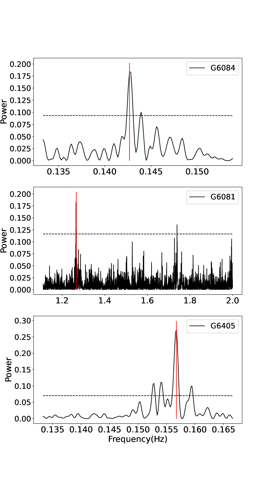
We collected multi-band LCs from current wide-field photometric TD surveys, and tried to estimate the orbital periods by using the Lomb-Scargle method (VanderPlas 2018). The periods of G6084, G6081, and G6405 were estimated as $\approx$ 7.00880 day, 0.78951 day, and 6.38246 days, respectively (Figure 6), which were similar to those values derived with RV data.

The LCs (Figure 7, 8 and 9), folded with the periods estimated from RV data, show typical double-peaked morphology expected for a tidally distorted secondary. The two asymmetrical peaks in folded LCs suggest an O’Connell effect (Wilsey & Beaky 2009), which may be caused by asymmetric distributed cool starspots (Linnell 1986), a hot spot located in an accretion disk (Andronov & Richter 1987), or clouds of circumstellar material (Liu & Yang 2003). For G6081 and G6405, the interchange between the two light maxima in different years are similar to the flip-flop behaviour, which is explained as two active longitudes about 180^o apart with alternating levels of spot activity (Korhonen et al. 2001). Although the LCs can help constrain the inclination angle, the precision of the data are too low to do the LC fitting.

V.2 The nature of the unseen object

For G6084, the luminosity of the visible star is about ( $3.52{\pm 0.09})\times 10^{34}$ erg/s. The minimum luminosity of the unseen object is about ( $2.64{\pm 0.06})\times 10^{33}$ erg/s following (Eker et al. 2018),

{\rm log}L=(5.743{\pm 0.413})\times{\rm log}M-(0.007{\pm 0.026}),

(9)

assuming the unseen object is an main-sequence star of 0.94 M_⊙. The luminosity of the visible star of G6081 is about ( $2.42{\pm 0.03})\times 10^{33}$ erg/s. Assuming that the unseen object is a dwarf of 0.69 or 0.76 M_⊙, the luminosity can be calculated as ( $5.55{\pm 0.22})\times 10^{32}$ erg/s or ( $7.79{\pm 0.29})\times 10^{32}$ following

{\rm log}L=(4.572{\pm 0.319})\times{\rm log}M-(0.102{\pm 0.076}).

(10)

For G6405, the luminosity of the visible star is about ( $3.40{\pm 0.02})\times 10^{34}$ erg/s. The minimum mass of the invisible star (0.69 or 0.81 M_⊙) leads to a minimum luminosity around ( $5.55{\pm 0.22})\times 10^{32}$ or ( $1.12{\pm 0.02})\times 10^{33}$ erg/s following Eq. 10. In previous studies, G6405 was classified as one RS CVn source due to its spotted feature (Drake et al. 2014).

For all these three sources, the inferred luminosity of the invisible star is about one tenth of the visible star. Although no obvious double-line feature is seen from the LAMOST MRS spectra of the three sources, it’s more reasonable to check the binarity of these spectra with the spectral disentangling method.

V.2.1 Spectral disentangling

We used the algorithm of spectral disentangling proposed by Simon & Sturm 1994. For G6081, the maximum mass ratio ( $q=M_{\rm 1}/M_{\rm 2}$ ) is around 1, indicating a secondary with mass close to or larger than that of the primary (which is a main-sequence star). The secondary component can be clearly distinguished from the observed spectra if it’s a normal star. Therefore, we only did spectral disentangling for G6084 and G6405.

We first did some test to check the detection limit of the secondary star with this method for our sources. According to the mass ratio $q$ in Table 5, we derived approximate effective temperature and surface gravity of the secondary (assuming a main-sequence star) with its minimum mass⁵⁵ 5 http://www.pas.rochester.edu/ẽmamajek/EEM_dwarf_UBV- IJHK_colors_Teff.txt. We picked out model templates from Phoenix⁶⁶ 6 https://phoenix.astro.physik.uni-goettingen.de, reduced their resolution to $R=$ 7500, and applied rotational broadening ( $v{\rm sin}i=$ 10 km/s, 50 km/s, 100 km/s and 150 km/s) and absorption. By combining those models with the observational spectra, we got a grid of faked binary spectra for the test. The spectral disentangling results by visual check are listed in Table 6. When $q$ is 0.8 and $v{\rm sin}i$ $<$ 100 km/s, this method can separate the binary components for both G6804 and G6405. When $q$ is 1.2, for G6804 the spectrum of the secondary can be distinguished but in low significance; for G6405 the spectra can’t be disentangled, mostly due to the low SNR of the faked spectra. Considering that the secondary mass in Table 5 is only the minimum value and the mass ratio will decrease as the inclination angle decreases, the disentangling method are still suitable for our targets, although the constraint on the nature of G6405’s secondary may be weak.

We used the spectrum wavelength ranging from 6400 Å to 6600 Å to disentangle the spectra. In order to try different sets of RV ratio, we sampled different mass ratio (from 0.8 to 1.2) through MCMC. The disentangling results are shown in Figure 10 and 11. No additional component with optical absorption spectrum can be detected, excluding the scenario of normal binary.

Table 6: Spectral disentangling results by visual check. ”✔✔” means the spectra are well disentangled, ”✔” means the spectra can be disentangled but in low significance, and ”✕” means the spectra can not be disentangled.

Object

q

v{\rm sin}i

Disentangling

results

G6084

0.8

✔✔

100

✔✔

150

1.0

✔✔

100

✔✔

150

1.2

✔

100

✔

150

G6405

0.8

✔✔

100

✔✔

150

1.0

✔

100

150

1.2

100

150

V.2.2 X-ray upper limit

The sky fields of the three sources have been covered by ROSAT during its X-ray sky survey, although without any detection of them. The observations were performed with the instrument Position Sensitive Proportional Counter (hereafter PSPC). Here we tried to give upper limit estimations of these sources by using the archival PSPC data.

For G6081 and G6405, we used the observations ObsID rp700887n00 and rs931310n00, respectively. The radius of the photometric aperture was set as 30^′′ and an annulus around it was used to estimate the background emission. For G6081, we obtained an upper limit of $\approx$ 0.00024 count s^-1 in the 0.2–8 keV range. The hydrogen column density $N_{\rm H}$ can be calculated following the standard linear relation between $N_{\rm H}$ and the reddening $N_{\rm H}=$ 5.8 $\times 10^{21}$ cm^-2 $E(B-V)$ . By using the WebPIMMS⁷⁷ 7 https://heasarc.gsfc.nasa.gov/cgi-bin/Tools/w3pimms/w3pimms.pl, we derived an unabsorbed flux of 5.7 $\times 10^{-15}\ \rm erg\,s^{-1}\,cm^{-2}$ in the 0.2–8 keV range assuming $\tau=$ 1.5 for a power-law spectrum, or 2.9 $\times 10^{-15}\ \rm erg\,s^{-1}\,cm^{-2}$ assuming $\tau=$ 2. At a distance $d=0.32\,$ kpc (Section III.1), the flux corresponds to a luminosity of $L_{X}$ $\lesssim$ 7.0 $\times$ 10²⁸ $\rm erg\,s^{-1}$ or 3.5 $\times$ 10²⁸ $\rm erg\,s^{-1}$ . For G6405, the upper limit count rate is about 0.000052 count s^-1. The estimated unabsorbed flux is around 2.4 $\times 10^{-15}\ \rm erg\,s^{-1}\,cm^{-2}$ ( $\tau=$ 1.5) or 1.8 $\times 10^{-15}\ \rm erg\,s^{-1}\,cm^{-2}$ ( $\tau=$ 2), corresponding to a luminosity of $L_{X}$ $\lesssim$ 1.1 $\times$ 10³⁰ $\rm erg\,s^{-1}$ or 8.5 $\times$ 10²⁹ $\rm erg\,s^{-1}$ .

For G6084, we used the observation Obsid rs931310n00 to determine the upper limit count rate. Due to the quite few photons, a larger radius (60^′′) was used to do the aperture photometry. A count rate of 0.000054 count s^-1 leads to an unabsorbed flux of 1.3 $\times 10^{-15}\rm erg\,s^{-1}\,cm^{-2}$ ( $\tau=$ 1.5) or 6.5 $\times 10^{-16}\rm erg\,s^{-1}\,cm^{-2}$ ( $\tau=$ 2). This corresponds to a luminosity of $L_{X}$ $\lesssim$ 1.9 $\times$ 10²⁹ $\rm erg\,s^{-1}$ or 9.4 $\times$ 10²⁸ $\rm erg\,s^{-1}$ .

V.2.3 UV emission

Both G6084 and G6081 have been observed by the Galaxy Evolution Explorer (hereafter GALEX). For G6084, the GALEX catalog presents a NUV magnitude of 19.22 $\pm$ 0.22 mag. The FUV magnitude of G6081 is 22.51 $\pm$ 0.18, however, the GALEX catalog doesn’t present a NUV magnitude due to the contamination of one nearby bright star.

We tried to do the aperture photometry using the Python module Photutils. The magnitudes were estimated with the formulae⁸⁸ 8 https://asd.gsfc.nasa.gov/archive/galex/FAQ/counts_back-
ground.html:

m_{\rm FUV,AB}=-2.5\times{\rm log10(Count\ Rate)}+18.82

(11)

and

m_{\rm NUV,AB}=-2.5\times{\rm log10(Count\ Rate)}+20.02.

(12)

The NUV magnitude of G6084 is 19.46 $\pm$ 0.02 mag; an upper limit of the FUV band was derived as 23.64 $\pm$ 1.14 mag, respectively. The FUV and NUV magnitudes of G6081 are 22.55 $\pm$ 0.26 and 18.35 $\pm$ 0.03 mag.

In addition, ROSAT consists one Wide Field Camera (WFC) covering the wavelength ranges of 60–140 Å and 110–200 Å. We investigated the ROSAT/WFC images for G6405 but no UV signal was found.

VI Summary

We presented the discovery of three binaries with possible compact components (i.e., G6084, G6081 and G6405) by using the LAMOST LRS and MRS data from our spectroscopic TD survey. G6084 is a binary with an orbital period of $P=$ 7.03 day containing a K-type subgiant. This visible primary has a mass of $\approx$ 1.18 $\pm 0.07$ M_⊙. By fitting the RV curve, we calculated the mass function of 0.19 M_⊙ and the minimum mass of the unseen secondary of 0.94 M_⊙. G6081 has an orbital period of $P=$ 0.79 day. The visible star is a G-type dwarf with a mass of $\approx$ 0.83 $\pm 0.01$ (or 0.69 $\pm 0.11$ ) M_⊙. The binary mass function is 0.17 M_⊙, and the minimum mass of the unseen object is estimated as $\approx$ 0.76 (or 0.69) M_⊙. G6405 is a binary with orbital period $P=$ 6.43 day. The visible star is a K-type subgiant with a mass of $\approx$ 1.00 $\pm 0.07$ (or 0.74 $\pm 0.08$ ) M_⊙. The mass function is 0.16 M_⊙. The compact object has a minimum mass of $\approx$ 0.81 (or 0.69) M_⊙. None of the visible stars has filled its Roche lobe.

The LCs and RVs show the same periods. However, due to the poor quality of the photometric data, we did not constrain the inclination angle of these binary systems. No double-line feature can be seen in the LAMOST medium-resolution spectra. Furthermore, we did spectral disentangling for our sources and found no additional component with absorption spectra, supporting the scenario that these sources are binary systems with compact components (i.e., including a white dwarf or neutron star). Note that the nature of the secondary of G6405 is weakly constrained by the spectral disentangling method, due to the low SNR of the observed spectra. The ROSAT data show no X-ray detection of these sources. The upper limits of X-ray luminosity of them range from 10²⁸ $\rm erg\,s^{-1}$ to 10³⁰ $\rm erg\,s^{-1}$ . Both G6048 and G6405 have bright UV counterparts, suggesting that they are more likely WDs rather than NSs.

Besides the four $K$ 2 plates, we are also carrying out a TD survey of another four $K$ 2 plates from 2020. More binaries containing compact objects can be found based on the LAMOST TD survey, which will help us in better understanding the late evolution of massive stars (in binaries).

acknowledgements

Guoshoujing Telescope (the Large Sky Area Multi-Object Fiber Spectroscopic Telescope LAMOST) is a National Major Scientific Project built by the Chinese Academy of Sciences. Funding for the project has been provided by the National Development and Reform Commission. LAMOST is operated and managed by the National Astronomical Observatories, Chinese Academy of Sciences. This work presents results from the European Space Agency (ESA) space mission Gaia. Gaia data are being processed by the Gaia Data Processing and Analysis Consortium (DPAC). Funding for the DPAC is provided by national institutions, in particular the institutions participating in the Gaia MultiLateral Agreement (MLA). The Gaia mission website is https://www.cosmos.esa.int/gaia. The Gaia archive website is https://archives.esac.esa.int/gaia. We acknowledge use of the VizieR catalogue access tool, operated at CDS, Strasbourg, France, and of Astropy, a community-developed core Python package for Astronomy (Astropy Collaboration, 2013). This research made use of Photutils Bradley et al. 2020, an Astropy package for detection and photometry of astronomical sources. This work was supported by National Science Foundation of China (NSFC) under grant numbers 11988101/11933004, National Key Research and Development Program of China (NKRDPC) under grant numbers 2019YFA0405504 and 2019YFA0405000, and Strategic Priority Program of the Chinese Academy of Sciences under grant number XDB41000000. S. W. and H.-L. Y. and acknowledges support from the Youth Innovation Promotion Association of the CAS (id. 2019057 and 2020060, respectively).

References

Abdul-Masih et al. (2020) Abdul-Masih, M., Banyard, G., Bodensteiner, J., et al. 2020, Nature, 580, E11, doi: 10.1038/s41586-020-2216-x
Andronov & Richter (1987) Andronov, I. L., & Richter, G. A. 1987, Astronomische Nachrichten, 308, 235, doi: 10.1002/asna.2113080403
Bailer-Jones et al. (2018) Bailer-Jones, C. A. L., Rybizki, J., Fouesneau, M., Mantelet, G., & Andrae, R. 2018, AJ, 156, 58, doi: 10.3847/1538-3881/aacb21
Bellm et al. (2019) Bellm, E. C., Kulkarni, S. R., Graham, M. J., et al. 2019, PASP, 131, 018002, doi: 10.1088/1538-3873/aaecbe
Bradley et al. (2020) Bradley, L., Sipőcz, B., Robitaille, T., et al. 2020, astropy/photutils: 1.0.0, 1.0.0, Zenodo, Zenodo, doi: 10.5281/zenodo.4044744
Casares et al. (2014) Casares, J., Negueruela, I., Ribó, M., et al. 2014, Nature, 505, 378, doi: 10.1038/nature12916
Chen et al. (2019) Chen, Y., Girardi, L., Fu, X., et al. 2019, A&A, 632, A105, doi: 10.1051/0004-6361/201936612
Cui et al. (2012) Cui, X.-Q., Zhao, Y.-H., Chu, Y.-Q., et al. 2012, Research in Astronomy and Astrophysics, 12, 1197, doi: 10.1088/1674-4527/12/9/003
Drake et al. (2009) Drake, A. J., Djorgovski, S. G., Mahabal, A., et al. 2009, ApJ, 696, 870, doi: 10.1088/0004-637X/696/1/870
Drake et al. (2014) Drake, A. J., Graham, M. J., Djorgovski, S. G., et al. 2014, ApJS, 213, 9, doi: 10.1088/0067-0049/213/1/9
Eggleton (1983) Eggleton, P. P. 1983, ApJ, 268, 368, doi: 10.1086/160960
Eker et al. (2018) Eker, Z., Bakış, V., Bilir, S., et al. 2018, in American Institute of Physics Conference Series, Vol. 2042, Turkish Physical Society 34th International Physics Congress (TPS34), 020016, doi: 10.1063/1.5078888
El-Badry & Quataert (2020) El-Badry, K., & Quataert, E. 2020, MNRAS, 493, L22, doi: 10.1093/mnrasl/slaa004
El-Badry et al. (2021) El-Badry, K., Quataert, E., Rix, H.-W., et al. 2021, MNRAS, 505, 2051, doi: 10.1093/mnras/stab1318
Gaia Collaboration et al. (2018) Gaia Collaboration, Brown, A. G. A., Vallenari, A., et al. 2018, A&A, 616, A1, doi: 10.1051/0004-6361/201833051
Green et al. (2015) Green, G. M., Schlafly, E. F., Finkbeiner, D. P., et al. 2015, ApJ, 810, 25, doi: 10.1088/0004-637X/810/1/25
Jayasinghe et al. (2021) Jayasinghe, T., Stanek, K. Z., Thompson, T. A., et al. 2021, MNRAS, 504, 2577, doi: 10.1093/mnras/stab907
Kochanek et al. (2017) Kochanek, C. S., Shappee, B. J., Stanek, K. Z., et al. 2017, PASP, 129, 104502, doi: 10.1088/1538-3873/aa80d9
Korhonen et al. (2001) Korhonen, H., Berdyugina, S. V., Strassmeier, K. G., & Tuominen, I. 2001, A&A, 379, L30, doi: 10.1051/0004-6361:20011359
Linnell (1986) Linnell, A. P. 1986, ApJ, 300, 304, doi: 10.1086/163804
Liu et al. (2020) Liu, C., Fu, J., Shi, J., et al. 2020, arXiv e-prints, arXiv:2005.07210. https://arxiv.org/abs/2005.07210
Liu et al. (2019) Liu, J., Zhang, H., Howard, A. W., et al. 2019, Nature, 575, 618, doi: 10.1038/s41586-019-1766-2
Liu & Yang (2003) Liu, Q.-Y., & Yang, Y.-L. 2003, Chinese J. Astron. Astrophys., 3, 142, doi: 10.1088/1009-9271/3/2/142
Luo et al. (2015) Luo, A. L., Zhao, Y.-H., Zhao, G., et al. 2015, Research in Astronomy and Astrophysics, 15, 1095, doi: 10.1088/1674-4527/15/8/002
Montet et al. (2015) Montet, B. T., Morton, T. D., Foreman-Mackey, D., et al. 2015, ApJ, 809, 25, doi: 10.1088/0004-637X/809/1/25
Morton (2015) Morton, T. D. 2015, isochrones: Stellar model grid package. http://ascl.net/1503.010
Price-Whelan et al. (2017) Price-Whelan, A. M., Hogg, D. W., Foreman-Mackey, D., & Rix, H.-W. 2017, ApJ, 837, 20, doi: 10.3847/1538-4357/aa5e50
Rivinius et al. (2020) Rivinius, T., Baade, D., Hadrava, P., Heida, M., & Klement, R. 2020, A&A, 637, L3, doi: 10.1051/0004-6361/202038020
Shenar et al. (2020) Shenar, T., Bodensteiner, J., Abdul-Masih, M., et al. 2020, A&A, 639, L6, doi: 10.1051/0004-6361/202038275
Simon & Sturm (1994) Simon, K. P., & Sturm, E. 1994, A&A, 281, 286
Swihart et al. (2021) Swihart, S. J., Strader, J., Aydi, E., et al. 2021, ApJ, 909, 185, doi: 10.3847/1538-4357/abe1be
Thompson et al. (2019) Thompson, T. A., Kochanek, C. S., Stanek, K. Z., et al. 2019, Science, 366, 637, doi: 10.1126/science.aau4005
VanderPlas (2018) VanderPlas, J. T. 2018, ApJS, 236, 16, doi: 10.3847/1538-4365/aab766
Wang et al. (2021) Wang, S., Zhang, H.-T., Bai, Z.-R., et al. 2021, Research in Astronomy and Astrophysics, 21, 292, doi: 10.1088/1674-4527/21/11/292
Wilsey & Beaky (2009) Wilsey, N. J., & Beaky, M. M. 2009, Society for Astronomical Sciences Annual Symposium, 28, 107
Zhao et al. (2012) Zhao, G., Zhao, Y.-H., Chu, Y.-Q., Jing, Y.-P., & Deng, L.-C. 2012, Research in Astronomy and Astrophysics, 12, 723, doi: 10.1088/1674-4527/12/7/002
Zong et al. (2020) Zong, W., Fu, J.-N., De Cat, P., et al. 2020, ApJS, 251, 15, doi: 10.3847/1538-4365/abbb2d

Appendix A LAMOST RV measurements for our targets.

Here we presented the LAMOST RV values used in this paper.

Table A.1: Barycentric-corrected RV values of G6084 from LAMOST observations.

BMJD	RV	Uncertainty	SNR	Resolution	BMJD	RV	Uncertainty	SNR	Resolution
(day)	(km/s)	(km/s)			(day)	(km/s)	(km/s)
58798.83429	52.78	0.7	21.12	MRS	58889.71963	30.27	0.65	19.14	MRS
58798.85096	53.28	0.6	16.7	MRS	58895.69519	32.77	0.65	19.51	MRS
58798.86694	52.78	0.75	10.01	MRS	58895.71117	32.27	0.65	19.53	MRS
58798.88291	54.28	0.8	8.2	MRS	58912.60353	118.32	0.55	40.35	MRS
58805.83359	47.78	0.65	17.98	MRS	58912.62019	118.82	0.55	35.22	MRS
58805.84956	48.78	0.6	23.16	MRS	58912.63617	119.82	0.6	33.16	MRS
58805.86623	49.28	0.65	21.79	MRS	58912.65214	120.83	0.6	28.52	MRS
58805.88221	50.78	0.6	20.14	MRS	58920.56694	149.34	0.65	23.29	MRS
58805.89818	50.28	0.7	18.67	MRS	58920.58292	149.34	0.7	16.45	MRS
58805.91485	51.78	0.6	17.07	MRS	58920.59889	149.84	0.8	10.51	MRS
58819.84877	47.28	0.6	24.04	MRS	58920.61833	147.84	1.05	6.64	MRS
58819.85780	47.78	0.6	26.67	MRS	58950.49786	96.81	0.55	28.81	MRS
58819.86752	47.78	0.6	26.04	MRS	58950.51383	95.81	0.55	24.26	MRS
58819.87655	48.28	0.6	23.53	MRS	58950.53050	94.31	0.6	22.73	MRS
58819.88627	48.28	0.6	21.42	MRS	59150.87673	81.3	0.55	23.03	MRS
58819.89530	49.78	0.6	21.61	MRS	59150.89271	81.8	0.6	26.57	MRS
58819.90433	49.78	0.6	23.9	MRS	59150.90649	81.8	0.7	7.85	MRS
58829.80167	147.34	0.65	15.89	MRS	59180.86159	151.84	0.65	20.32	MRS
58829.81140	146.84	0.6	17.62	MRS	59180.87826	151.84	0.6	26.94	MRS
58829.82043	148.34	0.65	14.62	MRS	59180.89424	152.85	0.65	17.17	MRS
58829.82945	147.34	0.65	16.6	MRS	59180.91021	151.34	0.7	14.02	MRS
58829.83918	146.34	0.65	15.73	MRS	59206.79000	64.29	0.65	25.64	MRS
58829.84821	146.34	0.7	16.19	MRS	59206.80598	64.79	0.65	29.24	MRS
58829.85793	146.34	0.65	15.97	MRS	59206.82264	65.79	0.65	28.21	MRS
58861.72151	35.77	0.65	19.16	MRS	59206.83862	66.79	0.6	30.15	MRS
58861.73749	36.77	0.65	18.87	MRS	59206.85459	68.29	0.65	29.84	MRS
58861.75415	36.27	0.65	20.58	MRS	59237.67106	144.84	0.6	18.25	MRS
58861.77013	37.27	0.65	17.66	MRS	59237.68773	143.84	0.65	17.6	MRS
58861.78610	37.77	0.65	19.11	MRS	59237.70370	143.34	0.75	8.61	MRS
58861.80277	38.77	0.65	18.6	MRS	59237.71967	144.34	0.6	18.4	MRS
58883.65859	75.8	0.6	29.5	MRS	59237.75995	141.84	0.65	16.48	MRS
58883.67457	77.3	0.55	28.01	MRS	59263.61317	92.81	0.6	13.64	MRS
58883.69123	77.8	0.55	26.38	MRS	59263.62915	93.81	0.6	15.04	MRS
58883.70720	77.8	0.55	24.04	MRS	59263.64512	94.31	0.6	18.36	MRS
58883.72387	78.8	0.55	25.5	MRS	59263.66178	94.81	0.55	22.23	MRS
58889.67102	29.27	0.7	17.43	MRS	59263.67775	96.31	0.55	24.79	MRS
58889.68699	29.27	0.7	15.13	MRS	59271.62953	137.84	0.75	10.52	MRS
58889.70297	30.27	0.7	17.71	MRS

Table A.2: Barycentric-corrected RV values of G6081 from LAMOST observations.

BMJD	RV	Uncertainty	SNR	Resolution	BMJD	RV	Uncertainty	SNR	Resolution
(day)	(km/s)	(km/s)			(day)	(km/s)	(km/s)
58837.76259	180.36	2.95	14.59	LRS	58912.62026	116.32	1.4	8.75	MRS
58837.77231	175.36	2.9	14.75	LRS	58912.63624	128.33	1.35	10.11	MRS
58837.78134	180.36	2.75	15.29	LRS	58912.65221	140.84	1.7	7.5	MRS
58843.73242	-44.28	2.6	17.26	LRS	59150.87661	-46.28	1.1	31.64	MRS
58843.75117	-36.27	2.35	19.18	LRS	59150.89258	-52.78	0.95	36.94	MRS
59191.85897	20.26	1.55	58.56	LRS	59150.90636	-61.79	1.45	12.31	MRS
59191.86799	10.76	1.5	61.26	LRS	59180.86148	-23.76	1.05	25.34	MRS
59191.87772	1.25	1.45	65.06	LRS	59180.87815	-33.77	0.95	32.24	MRS
58819.84866	-32.77	8.25	3.27	MRS	59180.89412	-45.78	1.05	21.31	MRS
58883.65860	144.84	1.15	8.86	MRS	59180.91010	-51.78	1.15	17.18	MRS
58883.67457	134.33	1.1	11.94	MRS	59206.78993	107.82	0.95	32.79	MRS
58883.69124	117.32	1.1	12.07	MRS	59206.80590	90.81	1.0	36.48	MRS
58883.70721	104.32	1.2	9.35	MRS	59206.82257	76.3	0.95	37.39	MRS
58912.60360	95.31	1.05	19.74	MRS

Table A.3: Barycentric-corrected RV values of G6405 from LAMOST observations.

BMJD	RV	Uncertainty	SNR	Resolution	BMJD	RV	Uncertainty	SNR	Resolution
(day)	(km/s)	(km/s)			(day)	(km/s)	(km/s)
58801.71828	-47.78	1.05	5.47	MRS	58890.46206	-82.3	0.95	9.75	MRS
58801.73495	-50.28	1.05	4.97	MRS	58890.47803	-82.8	0.95	9.97	MRS
58801.75092	-48.28	1.1	3.96	MRS	58890.49400	-80.8	0.9	9.03	MRS
58801.76674	-47.78	1.65	3.31	MRS	58890.51067	-82.8	0.95	7.99	MRS
58819.63005	-76.3	1.25	6.12	MRS	59123.78081	-16.26	1.15	4.29	MRS
58819.63908	-74.3	1.15	6.4	MRS	59123.79748	-5.25	1.5	4.66	MRS
58819.64810	-77.3	1.15	5.35	MRS	59123.81345	-10.76	1.7	3.94	MRS
58819.65783	-81.8	1.2	5.22	MRS	59123.83915	-3.75	2.45	3.06	MRS
58819.66685	-78.3	1.2	5.68	MRS	59147.72603	-78.3	1.6	3.97	MRS
58819.67588	-77.8	1.25	5.61	MRS	59147.75867	-81.3	1.85	3.27	MRS
58829.62353	49.28	1.65	3.04	MRS	59180.59676	-63.29	1.35	3.49	MRS
58829.63256	42.78	1.5	3.33	MRS	59180.61343	-59.79	1.6	3.22	MRS
58829.64228	42.28	1.5	3.37	MRS	59189.61118	46.28	1.1	7.07	MRS
58835.53361	34.77	1.55	3.82	MRS	59189.62785	42.78	2.05	5.01	MRS
58851.55712	-71.29	0.85	11.56	MRS	59189.64382	41.78	1.45	5.45	MRS
58851.57309	-71.79	0.85	11.66	MRS	59189.65979	44.28	1.4	4.74	MRS
58851.58975	-70.29	0.85	10.46	MRS	59189.67646	42.28	1.45	4.3	MRS
58851.60572	-71.29	0.95	11.26	MRS	59189.69243	46.78	1.4	3.99	MRS
58851.62239	-70.79	0.95	10.45	MRS	59215.57107	41.28	1.1	7.7	MRS
58883.47039	-64.79	1.45	3.26	MRS	59215.58704	36.27	1.05	7.16	MRS
58883.48636	-61.29	1.2	3.41	MRS	59215.60371	43.78	1.15	6.31	MRS
58883.50302	-70.29	1.3	3.39	MRS	59215.61968	39.27	1.15	6.78	MRS